Automatic Ship Detection in SAR Images Using Multi-Scale Heterogeneities and an A Contrario Decision

Abstract

The robust detection of ships is one of the key techniques in coastal and marine applications of synthetic aperture radar (SAR). Conventional SAR ship detectors involved multiple parameters, which need to be estimated or determined very carefully. In this paper, we propose a new ship detection approach based on multi-scale heterogeneities under the a contrario decision framework, with a few parameters that can be easily determined. First, multi-scale heterogeneity features are extracted and fused to build a heterogeneity map, in which ships are well highlighted from backgrounds. Second, a set of reference objects are automatically selected by analyzing the saliency of local regions in the heterogeneity map and then are used to construct a null hypothesis model for the final decision. Finally, the detection results are obtained by using an a contrario decision. Experimental results on real SAR images demonstrate that the proposed method not only works more stably for ships with different sizes, but also has better performance than conventional ship detectors.

1. Introduction

Ship detection in synthetic aperture radar (SAR) images has long been an active research topic and has many applications, such as monitoring of fishing activities and oil pollution, marine traffic management and crime control [1]. Due to multiple backscatter of the incoming radar waves from man-made objects, it becomes possible to separate ships from background clutters. However, the unique imaging mechanism of SAR makes it far more challenging [2], such as the bright spots induced by the coherence of the backscattered signal, the heterogeneities of sea clutter by different weather conditions and the unclear appearance of ships caused by different angle imaging in SAR imagery.

Many works have been devoted to target detection in SAR images. Among them, the constant false alarm rate (CFAR) detectors are mostly widely used. For example, the cell-averaged CFAR (CA-CFAR) and the order statistic CFAR (OS-CFAR) [3–6] are two classic one-parameter CFAR detectors; they are both considered to adaptively determine the detection threshold by using the statistics estimated from the boundaries of the detecting window. The background clutters are usually modeled by a Gaussian distribution. However, for complicated scenes, other models, such as Gamma, Weibull, K and Alpha-stable distribution, are recommended in [7–12], respectively. For these types of methods, it is computationally expensive to estimate the distribution parameters of complex distribution models, and the accuracy of parameter estimation also has significant influences on the final detection results. Furthermore, the pre-specified distribution models of background clutters may not fit the actual data well, especially in complicated scenes, which will degrade detection performance.

Another type of target detection method relies on the information extracted by image decomposition or transform [13–15], rather than statistical distribution models. In the work of Souyris et al. [13], a series of sublooks were generated from the single-look complex (SLC) image for inherent speckle effects analyses, and the internal Hermitian product (2L-IHP) was defined for target detection. In the approach proposed by Ouchi et al. [14], the cross-correlation values between two images extracted by small sliding windows from the multilook SAR intensity (or amplitude) images were used for detecting ship targets. Discrete wavelet transform was applied to SAR image by Tello et al. [15], and the difference of the statistical behavior of wavelet coefficients among ships and their surrounding sea clutters was utilized to provide reliable detection. Some other approaches are based on feature extraction and selection. The extended fractal feature, sensitive to both contrast and sizes of objects, was proposed to detect ships by Kaplan in [16]. In [17], genetic programming was introduced into target detection for SAR images by taking advantage of the “human vision system” approach to identify regions that stand out from their surroundings. The work of Bhanu et al. [18] focused on selecting discriminative features with a genetic algorithm, but the selected features cannot distinguish target and clutter well when the intensity of the clutter is stronger than targets. Our early work also tried to use the saliency map-based feature descriptor to pre-detect the object regions in SAR [19] and PolSAR images [20]. However, the performances of these feature mapping-based target detectors rely on setting suitable thresholds. Empiric thresholds are often deeply dependent on human judgment; thus, the quality of detection results varies with experimenters.

In this paper, we propose an automatic ship detection method that not only effectively highlights the targets by weakening the background clutters and speckle noise, but also accurately separates the targets from the background. The method dramatically decreases the false detection ratio for some small targets, while ensuring the accuracy of true detection. Unlike some work that mainly considers fitted statistical distribution models of background clutters or targets, we take the characteristics of the imaging mechanism of SAR and the physical characteristics of objects into consideration. Man-made objects always produce very strong scattering intensity in a wide azimuth, while background clutters cannot form such strong coherence with sub-pixel processing. Based on these facts, two techniques are introduced in our method; they are the multi-scale fused heterogeneity [19,20] feature extractor and the a contrario decision-based [21,22] target detector.

This paper is organized as follows. In Section 2, we first overview our ship detection approach, and we then introduce the heterogeneity feature extraction algorithm (Section 2.1) and the a contrario decision-based automatic target detector (Section 2.2), respectively. In Section 3, we study the performance of our models on ship detection for several SAR image datasets. We finally summarize our findings in Section 4.

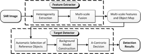
2. Our Algorithm

In this section, we first overview our new ship detection approach. The flowchart of detection is shown in Figure 1. The multi-scale fused heterogeneity measure is first designed to extract the heterogeneity map from the original SAR image, in which statistical discrepancies of ships and background clutter are enhanced. Then, a set of reference objects are automatically generated from the heterogeneity map by selecting regions with greater heterogeneity and by which the null hypothesis model of the a contrario decision is built. Finally, ships are detected by the a contrario decision procedure.

2.1. Heterogeneity Feature Extraction

The concept of heterogeneity for a SAR image is often ambiguous. In this paper, we define the heterogeneity feature of an object as the differences shown in appearance, structure or attribute, compared with other regions in the scene. To obtain good results, heterogeneity calculation should not only rely on prior information about the image under analysis [23], but also take advantage of the special imaging mechanisms of SAR images. The heterogeneity feature measured with the local image coefficient of variation by Lopes et al. [24] is sensitive to subtle discrepancies, such as speckle noise and bright clutters; while global heterogeneity measurements may cause the loss of detailed information of salient targets, such as global image statistics with Shannon’s information theory-based heterogeneity measurement, proposed by Bruno et al. [25]. We consider a novel framework of heterogeneity feature extraction by fusing local feature extractors and the global spatial information analysis. The works in [19,20] have revealed the effectiveness of the proposed framework in the task of salient object discovery from SAR images.

2.1.1. Heterogeneity Feature

In general, only textures of the radar cross-section (RCS) caused by artificial objects have clear geometric structures; the scattering intensity of a ship is stronger than that of its surroundings. This can be explained as heterogeneity.

For a SAR image X, we represent it with a set of non-overlapping patches, called local regions P = {p₁,⋯, p_n, ⋯, p_N}, (1 ≤ n ≤ N). Calculating heterogeneity involves comparing the differences between patches. Kullback–Leibler distance (KLD) is commonly used for measuring differences between statistic distributions of patches. In [26], Inglada et al. derived an analytical expression of KLD using cumulant-based approximation for SAR image change detection. Specifically, symmetric KLD of two regions p_i and p_j of X is defined as:

$$D(p_i,p_i)={\displaystyle \int \log \frac{f_i(x)}{f_j(x)}{f}_i(x)dx+{\displaystyle \int \log \frac{f_j(x)}{f_i(x)}{f}_j(x)}dx}$$

(1)

where f_i(x) is the probability density function (pdf) of the region i. The smaller this value, the more similar the statistics of the scattering characteristics of two regions are. We define the local heterogeneity of a test patch by calculating its cumulant-based KLDs (CKLD) to its neighbor patches. Let P_l be the l-th region surrounding one patch p_n, p_n ⊂ P, L is the number of these regions. The local heterogeneity of the patch p_n is defined as:

$$H_{lo}(p_n)=\frac{1}{L}{\displaystyle \sum _{l=1}^{L}D(p_n,p_l),}1\le l\le L$$

(2)

The patches belonging to background contain the basic information of the whole scene, typically exhibiting a strip- or block-like distribution, and often are locally homogeneous. Thus, a global heterogeneity feature can be extracted by comparing each test patch with background patches. The set of background patches Q = {q₁, q₂,⋯, q_K} is generated by the following steps: (1) select patches that are similar to most of the others; (2) to improve the purity of the candidate patches, select again to obtain more similar and adjacent patches in those selected ones. N/20 is a robust value for K. The similarities are defined by calculating CKLDs between any two patches. Then, the global heterogeneity for a region patch p_n is defined as:

$$H_{gb}(p_n)=\frac{1}{K}{\displaystyle \sum _{k=1}^{K}D}(p_n,q_k)$$

(3)

The local heterogeneity feature captures differences between local regions, while the global heterogeneity feature shows the saliency of the whole scene. They are complementary, and the final heterogeneity feature can be obtained by their product:

$$H(p_n)=H_{lo}(p_n)\cdot H_{gb}(p_n)$$

(4)

2.1.2. Multi-Scale Fusion

As we extract the heterogeneity features from patches, when using a large size of patches, fine structure information will be lost, while using small patches, the results will be noisy. In order to improve the accuracy and robustness of the algorithm, we take a multi-scale fusion strategy in heterogeneity feature extraction, by considering its dependence on various scales of local region patches [27]. With the heterogeneity features extracted in T scales R = {r₁,⋯r_t, ⋯, r_T}, (1 ≤ t ≤ T ), the local and global heterogeneity for patch p_n under each scale can be written as:

$$H_{lo}^{r_t}(p_n)=\frac{1}{L}{\displaystyle \sum _{l=1}^L{D}^{r_t}}(p_n,p_l),H_{gb}^{r_t}(p_n)=\frac{1}{K}{\displaystyle \sum _{k=1}^K{D}^{r_t}}(p_n,q_k)$$

(5)

Therefore, Equation (4) can be rewritten as:

$$H_t=H_{lo}^{r_t}\cdot H_{gb}^{r_t}$$

(6)

Here, heterogeneity features with T dimensions {H₁,⋯, H_T} are obtained.

The multi-scale fused heterogeneity H_fn is the weighted summation of heterogeneity features extracted in T scales:

$$H_{fn}={\displaystyle \sum _{t=1}^T\frac{r_1}{r_t}{H}_t}$$

(7)

For better performance, we normalize H_fn to [0, 1]. Gathering heterogeneity information under all scales together, the final heterogeneity feature H_fn forms the heterogeneity map.

2.2. A Contrario Decision-Based Ship Target Detection

Many adaptive threshold approaches have been proposed to extract targets from feature maps. Comparing to other parameter-setting or threshold-setting decision algorithms, the advantage of the a contrario decision is clear, as there is only one parameter that needs to be set. To obtain accurate decision, several a contrario decision-based algorithms [28–30] rely on the prior features or probability distribution models to build the null hypothesis model. These approaches can ensure reliable detection, but they also bring a problem of “how to assume the low false detection ratio when the prior information of a target or background is uncertain”. To handle this problem, we build a null hypothesis model based on a set of reference objects derived automatically from the heterogeneity map by using the statistics of the heterogeneity feature, rather than a pre-assumed a priori model. Thus, two key techniques are used in the proposed automatic target detector: a multi-scale fused heterogeneity measure is introduced to highlight targets from background clutters (see Section 2.1), and a contrario decision is applied to obtain the final detection results automatically.

2.2.1. A Contrario Decision

Considering a region B′ in the reference object set {B}, with a matching function F, an image I with N regions need to be tested. When a region Q ∈ I matching region B′ can be found, there are two explanations [31]:

• $\mathscr{H}$₀: the region Q matches with region B′ occasionally, but they are different actually.
• $\mathscr{H}$₁: indeed, the region Q matches with region B′, and they both describe one object.

A model for $\mathscr{H}$₁ can detect all targets accurately, but it is not feasible to build this model, because it requires complete information of the given object model and targets to be detected. Building the model for $\mathscr{H}$₀, called the null hypothesis model, is more practicable. As a decision can be made just based on the probability model of given objects for hypothesis $\mathscr{H}$₀, the decisions of $\mathscr{H}$₁ and $\mathscr{H}$₀ are obtained by comparing the matching results F (B′, Q) with a threshold value δ; accepting hypothesis $\mathscr{H}$₁ whenever F (B′, Q) < δ and rejecting hypothesis $\mathscr{H}$₁ whenever F (B′, Q) ≥ δ conversely. The quality of the decision relies on the probability of false decision. Here are two types of possible errors: accept $\mathscr{H}$₁ while $\mathscr{H}$₁ is false (false-positive, FP, Type I error), and $\mathscr{H}$₁ is rejected while $\mathscr{H}$₁ is actually true (false-negative, FN, Type II error). The probability of false-positive detections (PFP) and that of false-negative detections (PFN) can be written as:

$$PFP(B^{\prime },\delta )\equiv P_r(F(B^{\prime },Q)<\delta |{\mathscr{H}}_0)$$

(8)

$$PFN(B^{\prime },\delta )\equiv P_r(F(B^{\prime },Q)\ge \delta |{\mathscr{H}}_1$$

(9)

where P_r(·) is a probability function defined on the detection region Q.

The number of false-positive detections (NFP) in reference region B′ under the threshold value δ is:

$$NFP(B^{\prime },\delta )\equiv N\cdot PFP(B^{\prime },\delta )$$

(10)

which means the expected number of objects in the image whose matching result to B′ is below δ, when it is assumed that Σ obeys the hypothesis probability model. Thus, NFP(B′, F (B′, Q)) is the number of false-positive detections between reference region B′ and a region Q to be detected.

The ε-meaningful match is defined as: region Q is ε-meaningful matching with the detection region B′, if:

$$NFP(B^{\prime },F(B^{\prime },Q))\le \epsilon$$

(11)

The ε-meaningful match decision can be called an a contrario decision. We can directly control the number of false-positive detections by parameter ε. It is the only parameter of the a contrario decision. To ensure a minimal false detection, just let ε = 1. The null hypothesis model of the a contrario decision is built under the hypothesis that the number of detection regions N is large enough; thus, 1/N is close to zero.

2.2.2. Ship Detection Based on an A Contrario Decision

The decision procedure focuses on “is this area a part of the targets” rather than “is this area a part of the background”. Therefore, reference objects are needed to describe real targets in the SAR image. In the heterogeneity map, the target regions usually have higher heterogeneity values than others, so they appear brighter. We assume that those regions with high intensity and different distribution characteristics are object regions. Specifically, we calculate the distribution characteristic E in every dimension of the heterogeneity feature set within non-overlapping patches, and the size of the patch is that of the largest scale r_T × r_T :

$$E={\displaystyle \sum _{x\in p_n}{(h(x)-{\alpha }_n)}^2}$$

(12)

where p_n is an observed patch, h(x) is the heterogeneity value of pixel x and α_n is the maximum heterogeneity value of all pixels within p_n. Those regions with significant distribution characteristics in every dimension of heterogeneity feature set can be selected as reference object regions. Even though this set may not cover all target regions, it is enough for the following detection steps, as it contains correct target regions.

The null hypothesis model for $\mathscr{H}$₀ is a probability function defined on detection regions. Denoted by the marginal probability P_r(·|$\mathscr{H}$₀), in a single dimension, it can be presented as:

$$P(B^{\prime },\delta )=P_r(F(B^{\prime },Q)<\delta |{\mathscr{H}}_0$$

(13)

The following conditions must be satisfied: (1) the features’ values of detection regions are bounded and belong to one metric space; and (2) the results of matching function F (B′, Q) must be mutually independent between different dimensions in the feature space. In practice, the detection region (patch) Q is described by a set of T features {H₁(Q),⋯, H_T (Q)}; each of them is in the range [0, 1] and mutually independent.

The matching function F_t for each dimension is defined by the Manhattan distance:

$$F_t(B^{\prime },Q)=|H_t(B^{\prime })-H_t(Q)|$$

(14)

The global distance of the complete feature space can be obtained by weighting each dimension of distances. To reduce the complexity of setting parameters, we define it in a simple way:

$$F_t(B^{\prime },Q)=\underset{t\in \{1,\cdots .T\}}{\max }(|S_t(B^{\prime })-S_t(Q)|)$$

(15)

The weights significantly influence matching and deciding results, so it is a harsh punishment to take the maximum distance as the ultimate distance. Simultaneously, the credibility of the reference object set is sharply increased.

Replacing the threshold value δ by the matching result F_t(B′, Q), the corresponding false alarm probability of meaningful detection is:

$${\delta }_t(B^{\prime },Q)=P_t(B^{\prime },F_t(B^{\prime },Q))=P_r(F_t(B^{\prime },\mathrm{\Sigma })<F_t(B^{\prime },Q)|{\mathscr{H}}_0)$$

(16)

Finally, the product matching result under multi-dimension features is:

$$F(B^{\prime },Q)=\underset{t\in \{1,\cdots ,T\}}{\max }{\delta }_t{(B^{\prime },Q)}^T$$

(17)

Additionally, the number of false-positive detections in reference B′ is:

$$NFP(B^{\prime },Q)=N\cdot F(B^{\prime },Q)$$

(18)

Thus, the quality of the decision relies on the credibility of the reference object set, rather than the size of the set.

3. Experimental Results

3.1. Datasets and Experimental Settings

The proposed ship detection algorithm is tested and analyzed on TerraSAR-X and RADARSAT-2 data, as shown in Figure 2. As no AIS (Automatic Identification System) information about the ships is available, the ground truth for performance evaluation is made by human visual interpretation. Ships are marked in red ellipses in Figure 3. In Figure 2a–d, the numbers of ships are 8, 9, 14 and 8, respectively. In Figure 2e–h, there are 9, 28, 33 and 36 ships in them, respectively. All test images are 1000 × 1000 pixels. As we can see, for the former four SAR images, the scenes are relatively simple, with easily distinguished ships. The scenes of the latter four images are complex, with stronger background clutters, ship wakes and ghosts relative to the corresponding true ships, and the sizes of ships are also very different, which make it difficult to detect all ships accurately.

In the stage of feature extraction, considering the different sizes of ships, heterogeneity features are extracted by calculating CKLDs between patches in multiple scales. The sizes of patches vary from 4×4 to 21 × 21 pixels with four scales. Three widely-used CFAR detectors are implemented for comparison, in which background clutters are modeled by Nakagami [32], Weibull [8] and G′ [33] distributions, respectively. The parameters for these three CFAR detectors (Nakagami-CFAR, Weibull-CFAR and G′-CFAR) are as follows: the size of detection window is 21 × 21 pixels (equals the largest size of patches for the proposed approach); the size of the target window is 3 × 3 pixels (smaller than the smallest size of patches for the proposed approach); the size of alerting region is three pixels; and the false alarm rate is 0.0001. The detected ships of these three algorithms are shown in white to heighten their legibility in their result maps. For the proposed approach, since the detection results stage is carried out on the heterogeneity map, the detection results are marked on feature map (H_fn) directly.

3.2. Results and Analysis

We divide our experimental images into two groups according to the scene complexity: the first group is the SAR images with a relatively simple scene, as shown in the first row of Figure 2, and the second group is the remaining four SAR images with a complex scene.

We first test our algorithm on the images with a simple background. The heterogeneity feature extraction algorithm is first carried out on these images, and the feature maps are shown in Figure 4. These maps clearly describe the heterogeneity of the scene, and the significant objects stand out, even small and insignificant objects have not been ignored. What is more, the feature extractor filters most of the ship ghosts and background clutters. As seen in Figure 4c, the speckle noise has little effect on the mapping results, which is bright in the original image. After feature extraction, the most salient ships are selected as reference object regions. At last, the ships can be detected with the accurate reference set and the a contrario decision model. To compare with the other three algorithms, the detection results for different SAR images with all four different algorithms are shown in Figure 5. Figure 5b–d show the results of Nakagami-CFAR, Weibull-CFAR and G′-CFAR algorithms, respectively. For better comparison, detected objects of these three CFAR detectors are marked in white boxes. In these results, most of ship targets are detected, but there are also some false targets. In the result of Nakagami-CFAR, most of the ship targets are successfully detected. However, the false alarm rate is high; many false targets are also detected, and the accuracy of detection is seriously affected by noise, particularly in the result of the third and forth SAR images (seen in the yellow rectangle in Figure 5). Weibull-CFAR achieves better results; its false-positive ratio is low, but there are still targets that are not detected completely. The detection results of the G′-CFAR algorithm have a lower false-positive ratio, but some true targets are missed, such as the yellow ovals marked in the results of the second SAR images. The detection results of the proposed approach are shown in the fifth column of Figure 5. Most ship targets are well detected and correctly located. Some fake targets are shown in the feature maps, but the a contrario decision model does not make false decisions. Thus, the number of false-positive detections of our approach is zero in these simple images. Note that, detected targets of the proposed approach are automatically marked in white boxes, with the a contrario decision.

The quantitative evaluations are shown in

Table 1. Comparison of different detection algorithms in SAR images with a simple scene.

Algorithm			Performance
Image Figure 2a	Ntt	Nfp	Nfn	Pd	Pq
Nakagami-CFAR	8	3	0	100%	72.73%
Weibull-CFAR	8	3	0	100%	72.73%
G′-CFAR	8	0	0	100%	100%
The proposed approach	8	0	0	100%	100%
Image Figure 2b	Ntt	Nfp	Nfn	Pd	Pq
Nakagami-CFAR	9	3	0	100%	75.00%
Weibull-CFAR	9	6	0	100%	60.00%
G′-CFAR	8	0	1	88.89%	88.89%
The proposed approach	9	0	0	100%	100%
Image Figure 2c	Ntt	Nfp	Nfn	Pd	Pq
Nakagami-CFAR	12	22	2	85.71%	33.33%
Weibull-CFAR	12	2	2	85.71%	75.00%
G′-CFAR	12	0	2	85.71%	85.71%
The proposed approach	14	0	0	100%	100%
Image Figure 2d	Ntt	Nfp	Nfn	Pd	Pq
Nakagami-CFAR	8	21	0	97.43%	27.59%
Weibull-CFAR	7	1	1	94.87%	77.78%
G′-CFAR	6	0	2	75.00%	75.00%
The proposed approach	8	0	0	100%	100%

. Two measures, the accuracy of detection P_d and the quality factor P_q, are calculated as:

$$P_d=\frac{N_{tt}}{N_T},P_q=\frac{N_{tt}}{N_T+N_{fp}}$$

(19)

where N_tt is the number of targets correctly detected, N_T is the number of true targets in the SAR image, N_fp is the number of false-positive detected targets and N_fn is the number of false-negative detected targets. Though we set a low false alarm rate (0.0001), the amounts of false-positive detected targets for the three traditional CFAR detectors are still high, resulting in low P_q values. This is because their detection performances are also dependent on other parameters, like the size of the detection window, guard region, etc., which are specified empirically. On the contrary, as shown in Figure 5e, the proposed algorithm relies on a few parameters. Meanwhile, the proposed heterogeneity measure can weaken the impact of speckle noise, even filter ship wakes and highlight ship targets from background clutters, which makes the following automatic decision more efficient.

In the results of the Nakagami-CFAR, Weibull-CFAR and G′-CFAR detectors shown in Table 1, the values of N_tt and the false-negative detections (N_fn) do not much of a difference. However, the numbers of false-positive detected N_fp are quite different. As these three CFAR detectors use the same configuration, the difference in performances comes from the models of the background clutter. This implies that the Weibull distribution is more suitable for the former two image groups, and the G′ distribution has better performance than the other two in these images. Not surprisingly, when the pre-assumed model of background clutters departs from the actual data, the performance of the CFAR detectors degrades. While the proposed approach achieves a better performance, higher P_d and P_q are achieved in these images.

In the second group of test images, there are much more ships, with a more complex background. The difficulties of successful detection in these images come from two aspects. First, the various types of ships and the sea clutter increase the complexity of the background; it is difficult to model the behavior of background clutter by a simple statistical distribution. Second, trails of moving ships and the reefs around often have high-angle scattering intensity, which also influences the detection of ship targets. Figure 6 shows the heterogeneity feature maps of the images. Besides ship targets, bright spots with high scattering intensity are also detected; they may be ship wakes or reefs. However, the fake targets have lower heterogeneity values than the true targets, as seen in the yellow circles marked in Figure 6a. Thus, the detection results are more accurate and have a lower false-positive detection rate.

Qualitative and quantitative evaluations are reported in Figure 7 and

Table 2. Comparison of different detection algorithms in SAR images.

Algorithm			Performance
Image Figure 2e	Ntt	Nfp	Nfn	Pd	Pq
Nakagami-CFAR	9	14	0	100%	29.13%
Weibull-CFAR	9	5	0	100%	64.29%
G′-CFAR	9	5	0	100%	64.29%
The proposed approach	9	0	0	100%	100%
Image Figure 2f	Ntt	Nfp	Nfn	Pd	Pq
Nakagami-CFAR	22	2	6	78.57%	73.33%
Weibull-CFAR	22	3	6	78.57%	70.97%
G′-CFAR	23	2	5	82.14%	76.67%
The proposed approach	25	0	3	89.29%	89.29%
Image Figure 2g	Ntt	Nfp	Nfn	Pd	Pq
Nakagami-CFAR	32	3	1	96.97%	88.89%
Weibull-CFAR	30	3	3	90.91%	83.33%
G′-CFAR	32	3	1	96.97%	88.89%
The proposed approach	32	1	1	96.97%	94.12%
Image Figure 2h	Ntt	Nfp	Nfn	Pd	Pq
Nakagami-CFAR	31	4	5	86.11%	77.50%
Weibull-CFAR	33	8	3	91.67%	75.00%
G′-CFAR	33	9	3	91.67%	73.33%
The proposed approach	33	0	3	91.67%	91.67%

, respectively. For SAR images with a complex scene, the ship detection results with three CFAR detectors are similar. Note that some fake objects with higher scattering intensity are detected as ships in all three detectors, as seen in the yellow rectangles marked in Figure 7. The numbers of false-positive detected N_fp of Weibull-CFAR and G′-CFAR detectors are close to the N_fp value of the Nakagami-CFAR detector. Thus, the values of the two quantitative evaluation measures are almost the same for these detectors. This means that the differences between these distribution models have little influence on the results of ship detection in complex scenes.

Again, the proposed approach achieves better performance. We can see that most ships are well detected; the number of false-positive detections is very low, as well as higher P_d and P_q values are achieved. In addition, to achieve better results, the parameters of Nakagami-CFAR, Weibull-CFAR and G′-CFAR have to be carefully selected. However, this is not easy, since they involve a set of parameters that can only be determined by trial and error. For the proposed approach, however, few parameters need to be tuned. What is more, the multi-scale combination of heterogeneity measures enhances the targets and also depresses the noise of the background clutter, ship wakes and fake targets. All of these make the proposed method robust for ship detection in complex situations.

4. Conclusions

This paper addressed the problem of automatic ship detection in SAR images, which often suffer from strong background clutter and speckle noise. In contrast with existing work on this topic, which concentrated on building a prior background distribution model to reduce the influences of the noise and the disturbance, we suggested considering the relationship between objects and the backgrounds, by investigating the imaging mechanism of SAR and the physical characteristics of objects. Specifically, we first introduced the heterogeneity feature extractor, to highlight objects from backgrounds, by calculating the heterogeneity between patches from the local and global perspectives simultaneously. In order to obtain better performance, we proposed a multi-scale feature fusion method to form the final heterogeneity feature map. After that, we adopted the a contrario decision framework, to automatically find the ship targets, by matching each image patch with the set of reference objects that was derived from the heterogeneity feature map. By experimenting on two groups of SAR images, we demonstrated the feasibility and efficiency of the proposed ship detection model.

It is also interesting to observe that the proposed target detection model depends more on the dissimilarities between patches rather than on probability distribution models. Thus, this work also provides a potential framework to detect interesting regions in different scenes, by incorporating different feature descriptors, similarity measures and decision-making models. In the current work, we demonstrated the use of the heterogeneity feature descriptor and the a contrario decision model, and further investigation of them is also of great interest, such as extending the work to detect targets from polarimetric SAR images.

References

- Margarit, G.; Barba Milanés, J.A.; Tabasco, A. Operational ship monitoring system based on synthetic aperture radar processing. Remote Sens 2009, 1, 375–392. [Google Scholar]
- Hu, C.; Ferro-Famil, L.; Kuang, G. Ship discrimination using polarimetric SAR data and coherent time-frequency analysis. Remote Sens 2013, 5, 6899–6920. [Google Scholar]
- Finn, H.; Johnson, R. Adaptive detection mode with threshold control as a function of spatially sampled clutter-level estimates. RCA Rev 1968, 29, 414–464. [Google Scholar]
- Hansen, V. Constant false alarm rate processing in search radars. Proceedings of the Radar Present Future, London, UK, 23–25 October 1973; pp. 325–332.
- Hansen, V.; Sawyers, J. Detectability loss due to “greatest of” selection in a cell-averaging CFAR. IEEE Trans. Aerosp. Electron. Syst 1980, 16, 115–118. [Google Scholar]
- Rohling, H. Radar CFAR thresholding in clutter and multiple target situations. IEEE Trans. Aerosp. Electron. Syst 1983, 19, 608–621. [Google Scholar]
- Kuruoglu, E.; Zerubia, J. Modeling SAR images with a generalization of the Rayleigh distribution. IEEE Trans. Image Process 2004, 13, 527–533. [Google Scholar]
- Levanon, N.; Shor, M. Order statistics CFAR for Weibull background. IEEE Proc. F Radar Signal Process 1990, 137, 157–162. [Google Scholar]
- Kuttikkad, S.; Chellappa, R. Non-Gaussian CFAR techniques for target detection in high resolution SAR images. Proceedings of the IEEE International Conference on Image Processing, Austin, TX, USA, 13–16 November 1994; 1, pp. 910–914.
- Armstrong, B.; Griffiths, H. CFAR detection of fluctuating targets in spatially correlated K-distributed clutter. IEEE Proc. F Radar Signal Process 1991, 138, 139–152. [Google Scholar]
- Alberola-López, C.; Casar-Corredera, J.; de Miguel-Vela, G. Object CFAR detection in Gamma-distributed textured-background images. IEEE Proc. Vis. Image Signal Process 1999, 146, 130–136. [Google Scholar]
- Wang, C.; Liao, M.; Li, X. Ship detection in SAR image based on the alpha-stable distribution. Sensors 2008, 8, 4948–4960. [Google Scholar]
- Souyris, J.; Henry, C.; Adragna, F. On the use of complex SAR image spectral analysis for target detection: Assessment of polarimetry. IEEE Trans. Geosci. Remote Sens 2003, 41, 2725–2734. [Google Scholar]
- Ouchi, K.; Tamaki, S.; Yaguchi, H.; Iehara, M. Ship detection based on coherence images derived from cross correlation of multilook SAR images. IEEE Geosci. Remote Sens. Lett 2004, 1, 184–187. [Google Scholar]
- Tello, M.; López-Martínez, C.; Mallorqui, J. A novel algorithm for ship detection in SAR imagery based on the wavelet transform. IEEE Geosci. Remote Sens. Lett 2005, 2, 201–205. [Google Scholar]
- Kaplan, L. Improved SAR target detection via extended fractal features. IEEE Trans. Aerosp. Electron. Syst 2001, 37, 436–451. [Google Scholar]
- Howard, D.; Roberts, S.; Brankin, R. Target detection in SAR imagery by genetic programming. Adv. Eng. Softw 1999, 30, 303–311. [Google Scholar]
- Bhanu, B.; Lin, Y. Genetic algorithm based feature selection for target detection in SAR images. Image Vis. Comput 2003, 21, 591–608. [Google Scholar]
- Huang, X.; Huang, P.; Dong, L.; Song, H.; Yang, W. Saliency detection based on distance between patches in polarimetric SAR images. Proceedings of the IEEE International Geoscience and Remote Sensing Symposium (IGARSS), Quebec City, QC, Canada, 13–18 July 2014; pp. 4572–4575.
- Huang, X.; Yang, W.; Yin, X.; Song, H. Saliency detection in SAR images. Proceedings of the European Conference on Synthetic Aperture Radar (EUSAR), Berlin, Germany, 3–5 June 2014; pp. 1–4.
- Musé, P.; Sur, F.; Cao, F.; Gousseau, Y.; Morel, J. An a contrario decision method for shape element recognition. Int. J. Comput. Vis 2006, 69, 295–315. [Google Scholar]
- Veit, T.; Cao, F.; Bouthemy, P. An a contrario decision framework for region-based motion detection. Int. J. Comput. Vis 2006, 68, 163–178. [Google Scholar]
- Aiazzi, B.; Baronti, S.; Alparone, L.; Cuozzo, G.; D’Elia, C.; Schirinzi, G. SAR image segmentation through information-theoretic heterogeneity features and tree-structured Markov random fields. IEEE Int. Geosci. Remote Sens. Symp 2005, 4, 2803–2806. [Google Scholar]
- Lopes, A.; Touzi, R.; Nezry, E. Adaptive speckle filters and scene heterogeneity. IEEE Trans. Geosci. Remote Sens 1990, 28, 992–1000. [Google Scholar]
- Aiazzi, B.; Alparone, L.; Baronti, S. Information-theoretic heterogeneity measurement for SAR imagery. IEEE Trans. Geosci. Remote Sens 2005, 43, 619–624. [Google Scholar]
- Inglada, J.; Mercier, G. A new statistical similarity measure for change detection in multitemporal SAR images and its extension to multiscale change analysis. IEEE Trans. Geosci. Remote Sens 2007, 45, 1432–1445. [Google Scholar]
- Xia, G.; Liu, G.; Yang, W. Meaningful Objects segmentation from SAR Images via A Multi-Scale Non-Local Active Contour Model. 2015. arxiv:1501.04163. arXiv.org e-Print archive Available online: http://arxiv.org/abs/1501.04163 accessed on 26 May 2015.
- Myaskouvskey, A.; Gousseau, Y.; Lindenbaum, M. Beyond independence: An extension of the a contrario decision procedure. Int. J. Comput. Vis 2013, 101, 22–44. [Google Scholar]
- Robin, A.; Moisan, L.; Hegarat-Mascle, L. An a contrario approach for subpixel change detection in satellite imagery. IEEE Trans. Pattern Anal. Mach. Intell 2010, 32, 1977–1993. [Google Scholar]
- Xia, G.; Delon, J.; Gousseau, Y. Accurate junction detection and characterization in natural images. Int. J. Comput. Vis 2014, 106, 31–35. [Google Scholar]
- Cao, F.; Lisani, J.L.; Morel, J.M.; Muse, P.; Frederic, S. A contrario decision: The LLD method. In A Theory of Shape Identification; Springer: Berlin/Heidelberg, Germany, 2008; Volume 1948, pp. 81–92. [Google Scholar]
- Moser, G.; Serpico, S. Generalized minimum-error thresholding for unsupervised change detection from SAR amplitude imagery. IEEE Trans. Geosci. Remote Sens 2006, 44, 2972–2982. [Google Scholar]
- Cheng, J.; Gao, G.; Ding, W.; Ku, X.; Sun, J. An improved scheme for parameter estimation of G′ distribution model in high-resolution SAR images. Prog. Electromagn. Res 2013, 134, 23–46. [Google Scholar]