
Performance of Linear and Nonlinear Two-Leaf Light Use Efficiency Models at Different Temporal Scales

 ,
,
Abstract
:
1. Introduction
2. Data and Methods
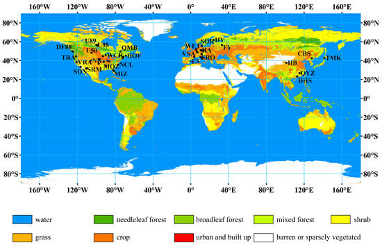
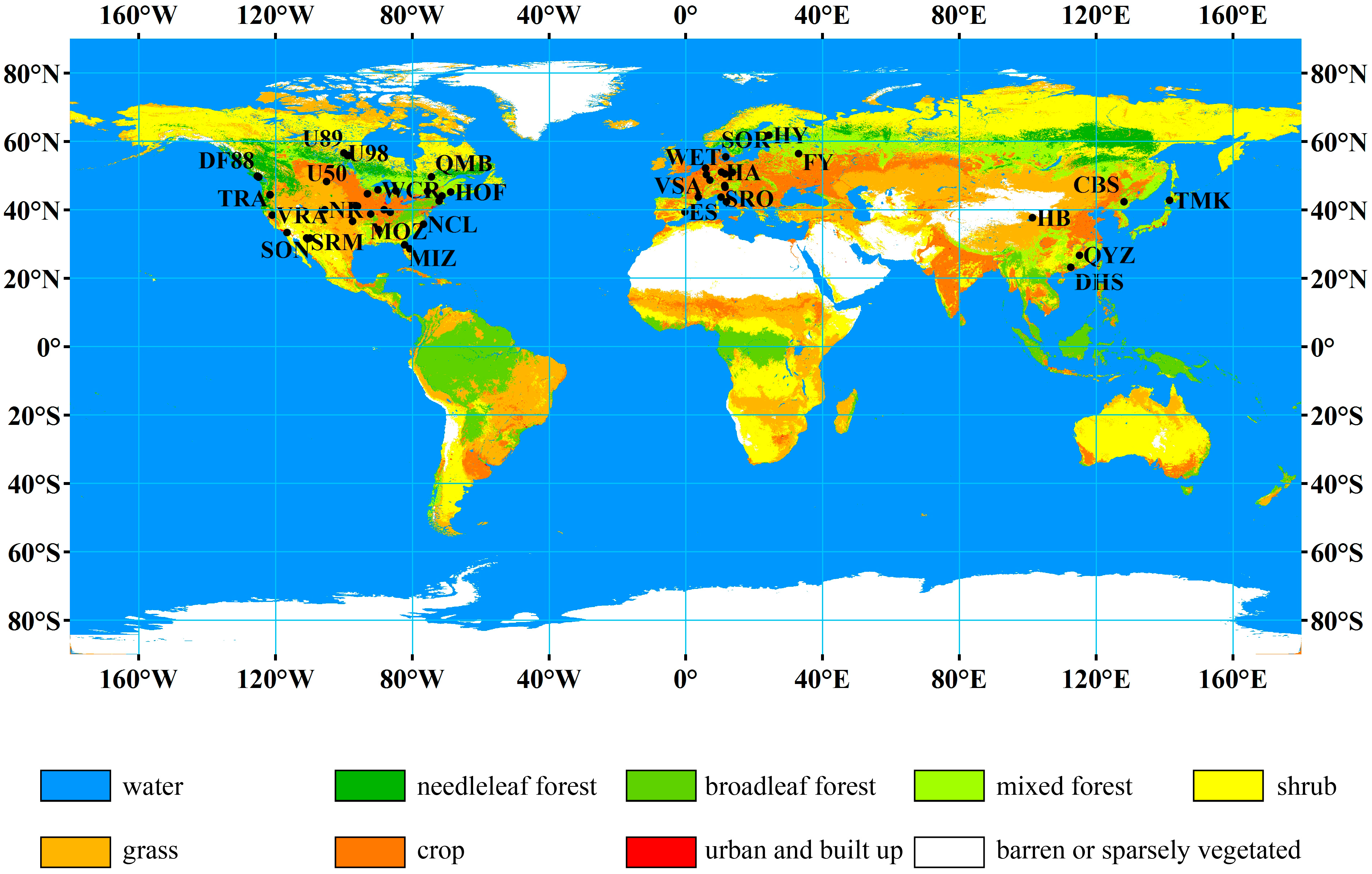
2.1. Data


| Site Name | Country | Lat. (°) | Long. (°) | Veg. Type | Opti. Years | Vali. Years | Reference |
|---|---|---|---|---|---|---|---|
| Austin Cary (ACA) | USA | 29.74 | −82.22 | NF | 2003 | 2005 | Gholz and Clark (2002) [42] |
| ARM_SGP_Main (ASM) | USA | 36.61 | −97.49 | CROP | 2003 | 2004 | Fischer et al. (2007) [43] |
| Audubon (AUD) | USA | 31.59 | −110.51 | GRASS | 2003 | 2004 | Wilson and Meyers (2007) [44] |
| BC-DFir1949 (BD49) | Canada | 49.87 | −125.33 | NF | 2003 | 2004 | Humphreys et al. (2006) [45] |
| Bartlett Experimental (BEP) | USA | 44.06 | −71.29 | BF | 2005 | 2006 | Jenkins et al. (2007) [46] |
| BC-Harvest Dfir2000 (DF00) | Canada | 49.87 | −125.29 | NF | 2003 | 2004 | Humphreys et al. (2006) [45] |
| BC-Harvest Dir1988 (DF88) | Canada | 49.53 | −124.9 | NF | 2004 | 2005 | Humphreys et al. (2006) [45] |
| Bondville (BON) | USA | 40.01 | −88.29 | CROP | 2004,2005 | 2006 | Wilson and Meyers (2007) [44] |
| Changbaishan (CBS) | China | 42.40 | 128.10 | MF | 2003 | 2004 | Zhang et al. (2006a,b) [47,48] |
| Dinghushan(DHS) | China | 23.17 | 112.53 | BF | 2003 | 2004 | Zhang et al. (2000) [49] |
| Donaldson (DON) | USA | 29.75 | −82.16 | NF | 2003 | 2004 | Gholz and Clark (2002) [42] |
| El Saler (ES) | Spain | 39.35 | −0.32 | NF | 2001,2002 | 2003 | Reichstein et al. (2006) [50] |
| Fort Peck (FPE) | USA | 48.31 | −105.1 | GRASS | 2003 | 2004 | Wilson and Meyers (2007) [44] |
| Fyodorovskoye (FY) | Russia | 56.46 | 32.92 | NF | 2001 | 2003 | Milyukova et al. (2002) [51] |
| Goodwin Creek (GCR) | USA | 34.25 | −89.87 | GRASS | 2004,2005 | 2006 | Wilson and Meyers (2007) [44] |
| Hainich (HA) | Germany | 51.08 | 10.45 | BF | 2001,2002 | 2003 | Mund et al. (2010) [52] |
| Harvard Forest (HAF) | USA | 42.54 | −72.17 | BF | 2005 | 2006 | Urbanski et al. (2007) [53] |
| Haibei (HB) | China | 37.67 | 101.33 | GRASS | 2003 | 2004 | He et al. (2013) [23] |
| Hesse (HES) | France | 48.67 | 7.07 | BF | 2001,2002 | 2003 | Granier et al. (2002) [54] |
| Howland Forest (HOF) | USA | 45.2 | −68.74 | MF | 2003 | 2004 | Hollinger et al. (1999, 2004) [55,56] |
| Hyytiala (HY) | Finland | 61.85 | 24.29 | NF | 2001 | 2002 | Kramer et al. (2002) [57] |
| Kendall (KED) | USA | 31.74 | −109.94 | GRASS | 2006 | 2007 | Scott (2010) [58] |
| Kennedy (KEN) | USA | 28.61 | −80.67 | SHRUB | 2004 | 2005 | Powell et al. (2006) [59] |
| Loobos (LOB) | Netherlands | 52.17 | 5.74 | NF | 2001,2002 | 2003 | Dolman et al. (2002) [60] |
| Mead Irrigated (MEI) | USA | 41.17 | −96.48 | CROP | 2003,2004 | 2005 | Verma et al. (2005) [61] |
| Mead Rainfed (MER) | USA | 41.18 | −96.44 | CROP | 2004 | 2005 | Verma et al. (2005) [61] |
| Metolius Intermediate (MIN) | USA | 44.45 | −121.56 | NF | 2005 | 2007 | Law et al. (2003) [62] and Thomas et al. (2009) [63] |
| Mead Irrigated Rotation (MIR) | USA | 41.16 | −96.47 | CROP | 2004 | 2005 | Verma et al. (2005) [61] |
| Mize (MIZ) | USA | 29.76 | −82.24 | SHRUB | 2003 | 2004 | Brocha et al. (2012) [64] |
| Morgan Monroe State (MMS) | USA | 39.32 | −86.41 | BF | 2003,2005 | 2006 | Schmid et al. (2000) [65] |
| Metolius New Young Pine (MNY) | USA | 44.32 | −121.6 | NF | 2004 | 2005 | Ruehr et al. (2012) [66] and Vickers et al. (2012) [67] |
| Missouri Ozark (MOZ) | USA | 38.74 | −92.2 | BF | 2005,2006 | 2007 | Gu et al. (2006) [68] |
| North Carolina Loblolly Pine (NCL) | USA | 35.8 | −76.67 | NF | 2005 | 2006 | Noormets et al. (2009) [69] |
| Neustift (NEU) | Austria | 47.12 | 11.32 | GRASS | 2002 | 2003 | Wohlfahrt et al. (2008) [70] |
| Niwot Ridge (NR) | USA | 40.03 | −105.55 | NF | 2003,2006 | 2007 | Monson et al. (2002) [71] |
| ON EpeatlandMerBleue (OEM) | Canada | 45.41 | −75.52 | SHRUB | 2001 | 2004 | Lafleur et al. (2003) [72] |
| Puechabon (PUE) | France | 43.74 | 3.6 | BF | 2001,2002 | 2003 | Allard et al. (2008) [73] |
| QC-Black Spruce (QMB) | Canada | 49.69 | −74.34 | NF | 2004 | 2005 | Bergeron et al. (2007) [74] |
| Qianyanzhou(QYZ) | China | 26.73 | 115.07 | NF | 2003 | 2004 | Yu et al. (2006) [75] |
| Renon (REN) | Italy | 46.59 | 11.43 | NF | 2002 | 2003 | Montagnani et al. (2009) [76] |
| Rosemount G19 (RG19) | USA | 44.72 | −93.09 | CROP | 2004,2005 | 2006 | Griffis et al. (2008) [77] |
| Rosemount G21 (RG21) | USA | 44.71 | −93.09 | CROP | 2004,2005 | 2006 | Bavin et al. (2009) [78] |
| Roccarespampani1 (ROC) | Italy | 42.39 | 11.92 | BF | 2002 | 2003 | Keenan et al. (2009) [79] |
| Sky Oaks New (SON) | USA | 33.38 | −116.64 | SHRUB | 2004,2005 | 2006 | Luo et al. (2007) [80] |
| Soroe (SOR) | Denmark | 55.48 | 11.65 | MF | 2001,2002 | 2003 | Pilegaard et al. (2001) [81] |
| Santa Rita Mesquite (SRM) | USA | 31.82 | −110.87 | SHRUB | 2004,2005 | 2006 | Scott (2010) [58] |
| San Rossore (SRO) | Italy | 43.73 | 10.29 | NF | 2001,2002 | 2003 | Migliavacca et al. (2011) [82] |
| Tharandt (THA) | Germany | 50.96 | 13.57 | NF | 2001,2002 | 2003 | Grünwald and Bernhofer (2007) [83] |
| Tomakomai (TMK) | Japan | 42.74 | 141.52 | NF | 2001,2002 | 2003 | Hirano et al. (2003) [84] |
| Tonzi Ranch (TRA) | USA | 38.43 | −120.97 | SHRUB | 2004,2005,2006 | 2007 | Baldocchi et al. (2004) [85] |
| UCI 1850 (U50) | Canada | 55.88 | −98.48 | NF | 2003 | 2004 | Goulden et al. (2011) [86] |
| UCI 1989 (U89) | Canada | 55.92 | −98.96 | SHRUB | 2003 | 2004 | Goulden et al. (2011) [86] |
| UCI 1998 (U98) | Canada | 56.64 | −99.95 | SHRUB | 2003 | 2004 | Goulden et al. (2011) [86] |
| UMBS (UMBS) | USA | 45.56 | −84.71 | BF | 2003,2004 | 2006 | Curtis et al. (2005) [87] |
| Vaira Ranch (VRA) | USA | 38.41 | −120.95 | GRASS | 2003,2004 | 2007 | Baldocchi et al. (2004) [85] |
| Vielsalm (VSA) | Belgium | 50.31 | 6.00 | MF | 2001,2002 | 2003 | Aubinet et al. (2001) [88] |
| Willow Creek (WCR) | USA | 45.81 | −90.08 | BF | 2003 | 2005 | Bolstad et al. (2004) [89] |
| Wetzstein (WET) | Germany | 50.45 | 11.46 | NF | 2002 | 2003 | Rebmann et al. (2009) [90] |
2.2. Methods
2.2.1. Models Used
| Vegetation Type* | DBF | ENF | EBF | MF | GRASS | CROP | savannas | OS | WS |
|---|---|---|---|---|---|---|---|---|---|
| εmax (g C/MJ)** | 1.044 | 1.008 | 1.259 | 1.116 | 0.604 | 0.604 | 0.888 | 0.774 | 0.768 |
| Tamin_max (°C) | 7.94 | 8.31 | 9.09 | 8.5 | 12.02 | 12.02 | 8.61 | 8.8 | 11.39 |
| Tamin_min (°C) | −8 | −8 | −8 | −8 | −8 | −8 | −8 | −8 | −8 |
| VPDmax (kpa) | 4.1 | 4.1 | 4.1 | 4.1 | 4.1 | 4.1 | 4.1 | 4.1 | 4.1 |
| VPDmin (kpa) | 0.93 | 0.93 | 0.93 | 0.93 | 0.93 | 0.93 | 0.93 | 0.93 | 9.3 |
| Albedo | 0.18 | 0.15 | 0.18 | 0.17 | 0.23a | 0.23b | 0.16 | 0.16 | 0.23 |
| Clumping index (Ωc) | 0.8 | 0.6 | 0.8 | 0.7 | 0.9 | 0.9 | 0.8 | 0.8 | 0.8 |
2.2.2. Parameter Optimization
2.2.3. Parameter Sensitivity Analysis
2.2.4. Model Performance Assessment
3. Results
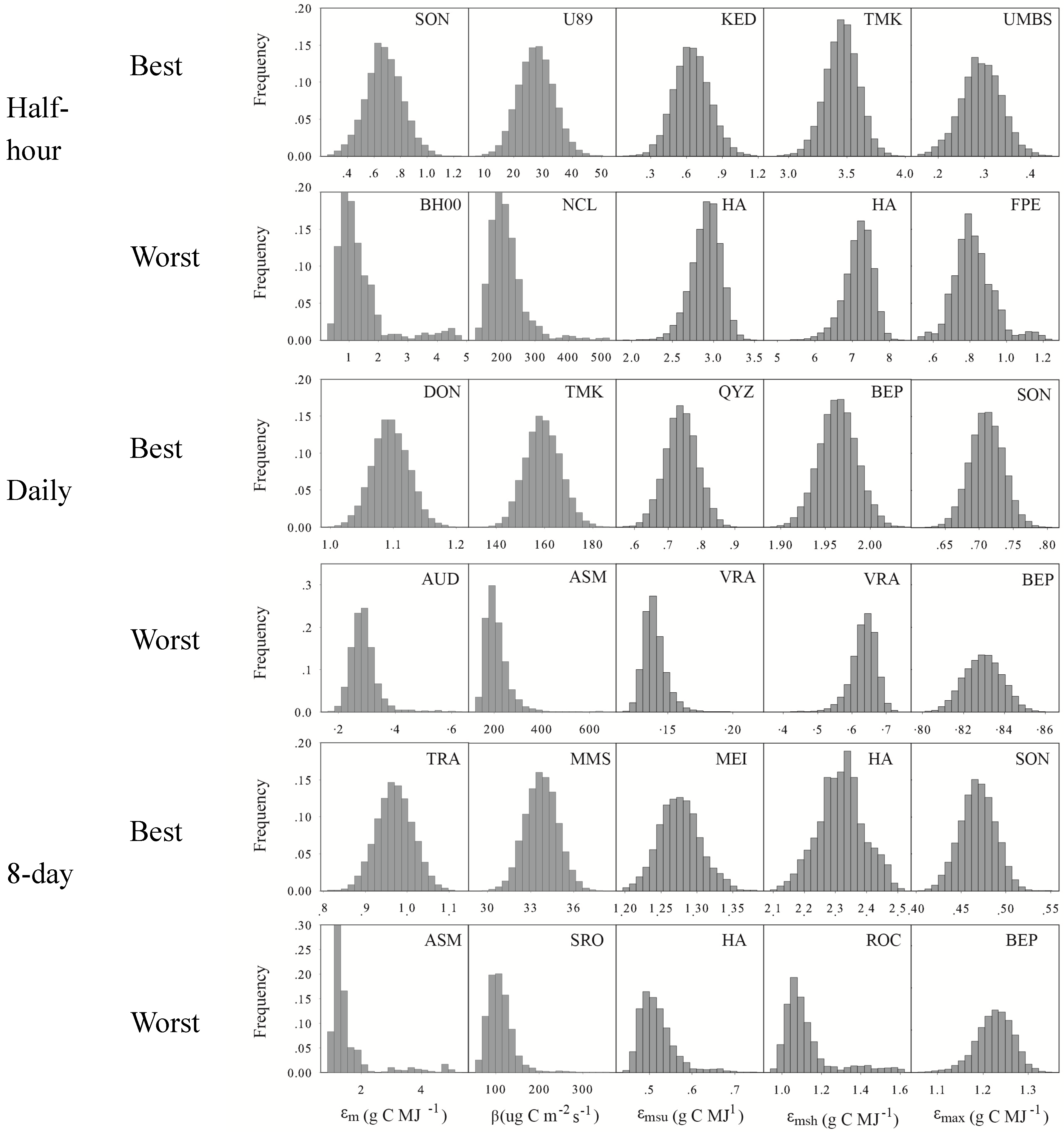
3.1. Optimized Model Parameters
| εm (g C MJ−1) | β (µg C m−2 s−1) | εmsu (g C MJ−1) | εmsh (g C MJ−1) | εmax (g C MJ−1) | ||||||||||||||||
|---|---|---|---|---|---|---|---|---|---|---|---|---|---|---|---|---|---|---|---|---|
| Mean | STD | CV (%) | Uncertainty | Mean | STD | CV(%) | Uncertainty | Mean | STD | CV(%) | Uncertainty | Mean | STD | CV(%) | Uncertainty | Mean | STD | CV(%) | Uncertainty | |
| Half-hourly | ||||||||||||||||||||
| BF | 3.52 | 1.72 | 48.93 | ±1.32 | 147.84 | 112.19 | 75.88 | ±77.50 | 0.58 | 0.15 | 25.20 | ±0.10 | 2.37 | 0.68 | 28.94 | ±0.39 | 0.88 | 0.24 | 27.39 | ±0.09 |
| CROP | 4.34 | 1.07 | 24.64 | ±1.46 | 470.48 | 235.03 | 49.96 | ±177.09 | 1.21 | 0.39 | 32.06 | ±0.16 | 5.23 | 1.90 | 36.34 | ±0.91 | 1.78 | 0.62 | 35.07 | ±0.16 |
| GRASS | 2.14 | 1.35 | 63.22 | ±1.13 | 273.55 | 333.25 | 121.83 | ±143.44 | 0.48 | 0.23 | 48.42 | ±0.16 | 1.69 | 1.06 | 62.74 | ±0.70 | 0.64 | 0.37 | 58.17 | ±0.14 |
| MF | 3.59 | 0.97 | 27.14 | ±1.27 | 214.63 | 83.46 | 38.89 | ±91.48 | 0.78 | 0.18 | 22.77 | ±0.13 | 3.33 | 0.83 | 24.91 | ±0.45 | 1.26 | 0.24 | 19.20 | ±0.11 |
| NF | 2.79 | 2.19 | 78.67 | ±0.92 | 308.14 | 272.11 | 88.31 | ±161.84 | 0.66 | 0.22 | 33.20 | ±0.16 | 2.35 | 0.79 | 33.57 | ±0.56 | 0.88 | 0.29 | 33.24 | ±0.11 |
| SHRUB | 2.41 | 3.48 | 144.64 | ±0.94 | 540.16 | 481.89 | 89.21 | ±242.72 | 0.53 | 0.17 | 32.29 | ±0.20 | 1.70 | 0.63 | 37.08 | ±0.95 | 0.65 | 0.24 | 36.44 | ±0.21 |
| Daily | ||||||||||||||||||||
| BF | 4.39 | 3.10 | 70.56 | ±1.05 | 99.88 | 93.92 | 94.04 | ±16.16 | 0.47 | 0.16 | 34.76 | ±0.02 | 2.06 | 0.63 | 30.47 | ±0.06 | 0.95 | 0.29 | 30.23 | ±0.02 |
| CROP | 12.02 | 5.05 | 42.06 | ±2.85 | 189.06 | 79.53 | 42.06 | ±23.26 | 0.95 | 0.30 | 31.47 | ±0.02 | 4.67 | 1.55 | 33.27 | ±0.12 | 1.80 | 0.58 | 32.19 | ±0.03 |
| GRASS | 6.06 | 5.94 | 98.14 | ±3.46 | 286.28 | 399.60 | 139.58 | ±143.94 | 0.44 | 0.26 | 58.18 | ±0.05 | 1.56 | 0.98 | 62.91 | ±0.17 | 0.69 | 0.44 | 63.51 | ±0.04 |
| MF | 3.41 | 0.73 | 21.48 | ±0.32 | 147.65 | 53.43 | 36.19 | ±14.80 | 0.61 | 0.14 | 22.19 | ±0.02 | 2.97 | 0.65 | 21.98 | ±0.06 | 1.40 | 0.26 | 18.76 | ±0.02 |
| NF | 2.69 | 1.79 | 66.53 | ±0.59 | 152.09 | 77.61 | 51.03 | ±36.93 | 0.54 | 0.15 | 28.38 | ±0.05 | 2.21 | 0.74 | 33.31 | ±0.11 | 0.98 | 0.32 | 32.24 | ±0.02 |
| SHRUB | 5.60 | 3.86 | 68.87 | ±5.13 | 105.57 | 51.30 | 48.59 | ±25.56 | 0.44 | 0.15 | 33.76 | ±0.05 | 1.84 | 0.64 | 34.68 | ±0.26 | 0.75 | 0.21 | 28.66 | ±0.05 |
| 8-day | ||||||||||||||||||||
| BF | 4.64 | 2.78 | 59.92 | ±1.37 | 163.58 | 271.85 | 166.19 | ±84.65 | 0.53 | 0.18 | 34.42 | ±0.11 | 1.83 | 0.59 | 32.27 | ±0.19 | 0.97 | 0.30 | 31.04 | ±0.05 |
| CROP | 14.79 | 5.21 | 35.26 | ±2.28 | 214.64 | 197.90 | 92.20 | ±82.78 | 0.96 | 0.27 | 27.95 | ±0.09 | 4.26 | 1.59 | 37.44 | ±0.31 | 1.80 | 0.58 | 32.00 | ±0.09 |
| GRASS | 3.19 | 3.93 | 123.31 | ±1.20 | 483.41 | 489.70 | 101.30 | ±192.63 | 0.48 | 0.29 | 59.81 | ±0.14 | 1.33 | 0.79 | 58.88 | ±0.28 | 0.70 | 0.45 | 64.58 | ±0.10 |
| MF | 2.39 | 0.38 | 15.97 | ±0.71 | 267.39 | 172.78 | 64.62 | ±150.71 | 0.79 | 0.18 | 22.48 | ±0.23 | 2.51 | 0.63 | 24.95 | ±0.31 | 1.45 | 0.27 | 18.64 | ±0.07 |
| NF | 2.31 | 1.66 | 71.68 | ±0.79 | 335.02 | 341.62 | 101.97 | ±206.24 | 0.68 | 0.25 | 36.09 | ±0.17 | 1.81 | 0.63 | 34.79 | ±0.28 | 1.01 | 0.34 | 33.65 | ±0.07 |
| SHRUB | 2.08 | 1.61 | 77.58 | ±1.19 | 369.31 | 399.01 | 108.04 | ±242.47 | 0.47 | 0.14 | 30.39 | ±0.14 | 1.62 | 0.77 | 47.12 | ±0.33 | 0.74 | 0.22 | 29.68 | ±0.13 |
3.2. Model Performance in Calibration Site-Years


3.3. Model Performance in Evaluation Site–years
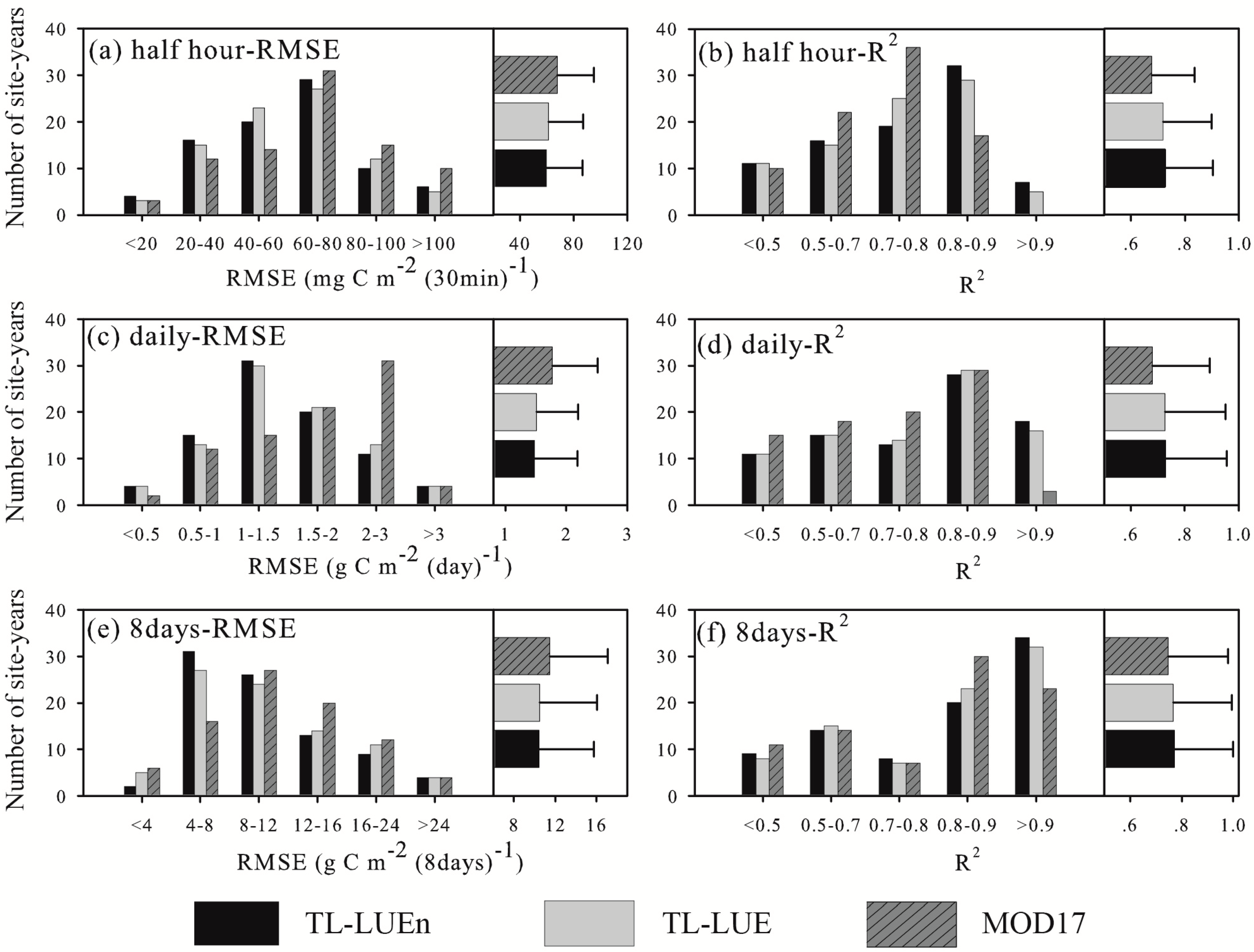
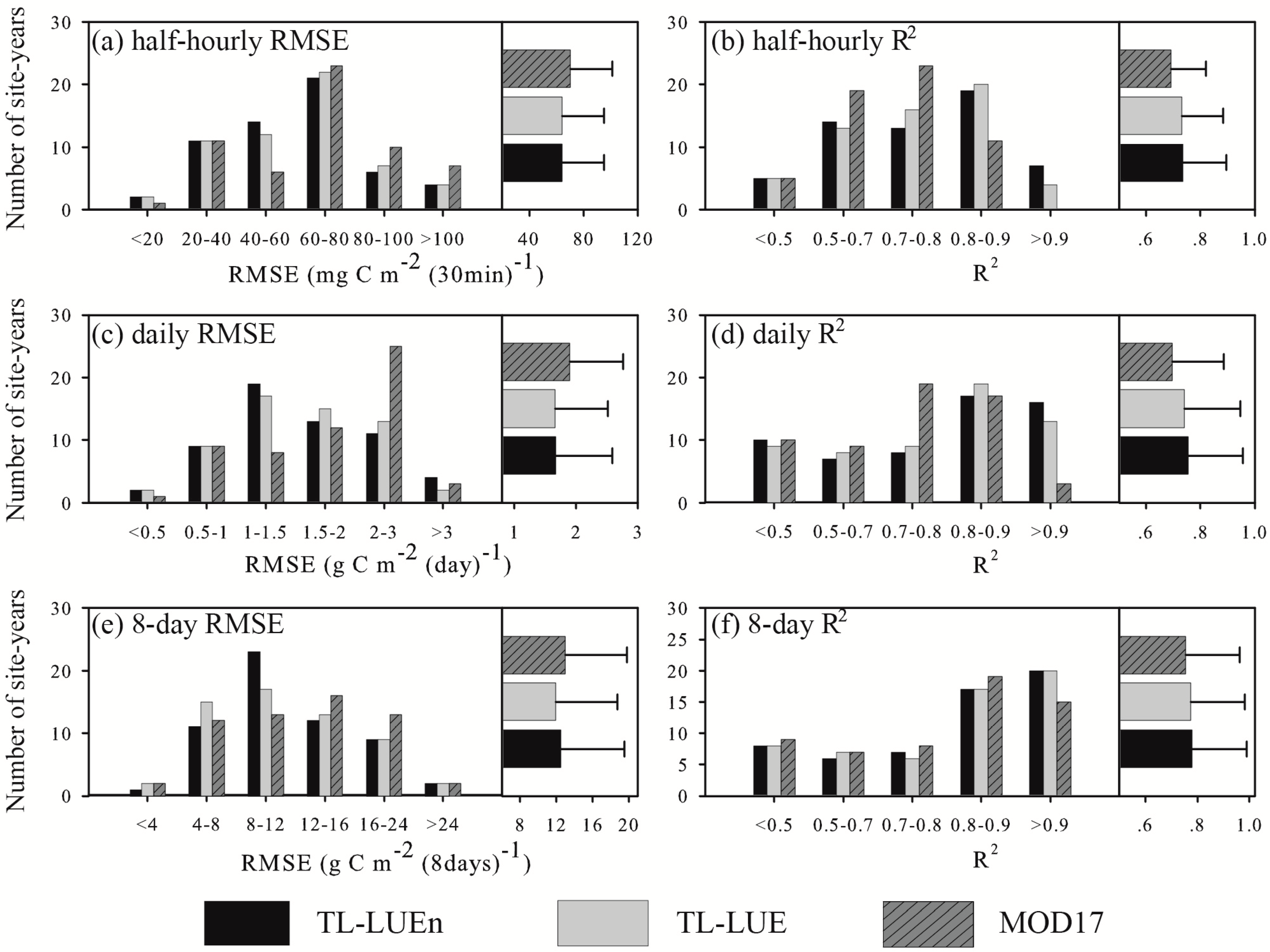
3.3.1. Model Performance at the Half-hourly Scale

| RMSE | R2 | |||||||
|---|---|---|---|---|---|---|---|---|
| TL-LUEn − TL-LUE | TL-LUEn − MOD17 | TL-LUE − MOD17 | TL-LUEn − TL-LUE | TL-LUEn − MOD17 | TL-LUE − MOD17 | |||
| Half-hourly | t stat | −0.75 | −4.33 | −5.09 | t stat | 1.12 | 6.10 | 7.13 |
| p | 0.45 | 0.00 | 0.00 | p | 0.27 | 0.00 | 0.00 | |
| Daily | t stat | 0.33 | −4.88 | −7.63 | t stat | 0.53 | 7.61 | 9.30 |
| p | 0.75 | 0.00 | 0.00 | p | 0.60 | 0.00 | 0.00 | |
| 8-day | t stat | 2.24 | −1.35 | −5.96 | t stat | 0.98 | 4.70 | 0.98 |
| p | 0.03 | 0.18 | 0.00 | p | 0.33 | 0.00 | 0.33 | |
3.3.2. Model Performance at the Daily Scale

3.3.3. Model Performance at the 8-day Scale
4. Discussion
4.1. The Ability of the Three LUE Models to Simulate GPP


4.2. The Applicability of Different Models

| Simulations | TL-LUEn | TL-LUE | MOD17 | ||||||
|---|---|---|---|---|---|---|---|---|---|
| εm | β | ΔGPPrel(%) | εmsu | εmsh | ΔGPPrel(%) | εmax | ΔGPPrel(%) | ||
| Half-hourly | 1 | - | - | −10.00 | - | - | −10.00 | - | −10.00 |
| 2 | + | - | 0.78 | + | - | −1.91 | |||
| 3 | - | + | −2.23 | - | + | 1.91 | |||
| 4 | + | + | 10.00 | + | + | 10.00 | + | 10.00 | |
| Main effect(%) | 11.50 | 8.50 | 8.09 | 11.91 | 20.00 | ||||
| Daily | 1 | - | - | −10.00 | - | - | −10.00 | - | −10.00 |
| 2 | + | - | 0.72 | + | - | −3.16 | |||
| 3 | - | + | −0.73 | - | + | 3.16 | |||
| 4 | + | + | 10.00 | + | + | 10.00 | + | 10.00 | |
| Main effect (%) | 10.72 | 9.28 | 6.84 | 13.16 | 20.00 | ||||
| 8-day | 1 | - | - | −10.00 | - | - | −10.00 | - | −10.00 |
| 2 | + | - | 0.60 | + | - | −2.48 | |||
| 3 | - | + | −1.92 | - | + | 2.48 | |||
| 4 | + | + | 10.00 | + | + | 10.00 | + | 10.00 | |
| Main effect (%) | 11.26 | 8.74 | 7.52 | 12.48 | 20.00 | ||||
4.3. Uncertainties and Remaining Issues
5. Conclusions
- (1)
- Optimized model parameters vary distinctly not only among different vegetation types, but also among different sites for the same vegetation type, especially for TL-LUEn. The parameters in TL-LUEn change sizably with temporal scales while the parameters in TL-LUE and MOD17 are almost invariant with temporal scales.
- (2)
- The overall performance of TL-LUEn was slightly but not significantly better than TL-LUE at half-hourly and daily scale, while the overall performance of both TL-LUEn and TL-LUE were significantly better (p < 0.0001) than MOD17 at the two temporal scales. The improvement of TL-LUEn over TL-LUE was relatively small in comparison with the improvement of TL-LUE over MOD17. However, the differences between TL-LUEn and MOD17, and TL-LUE and MOD17 became less distinct at 8-day scale.
- (3)
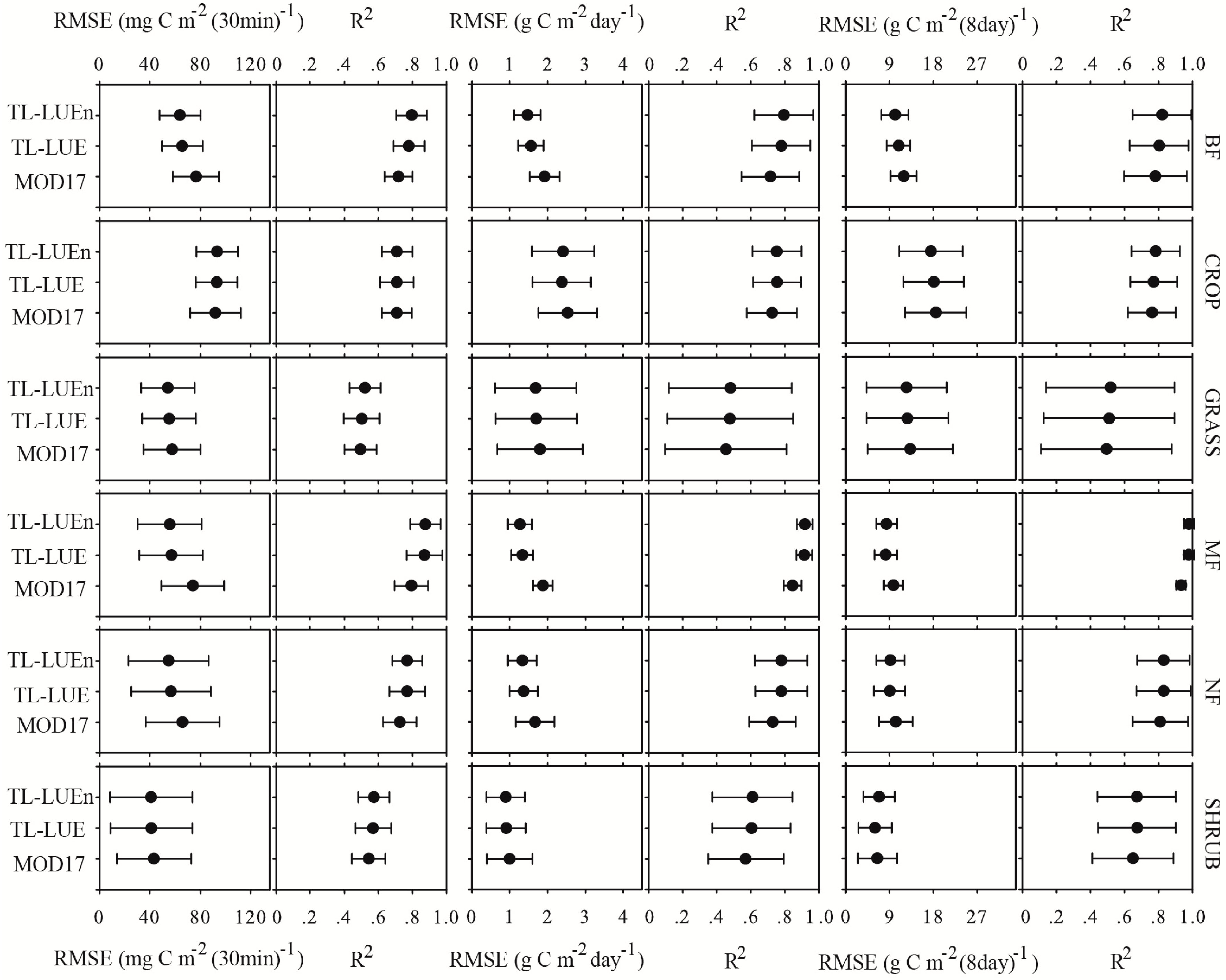
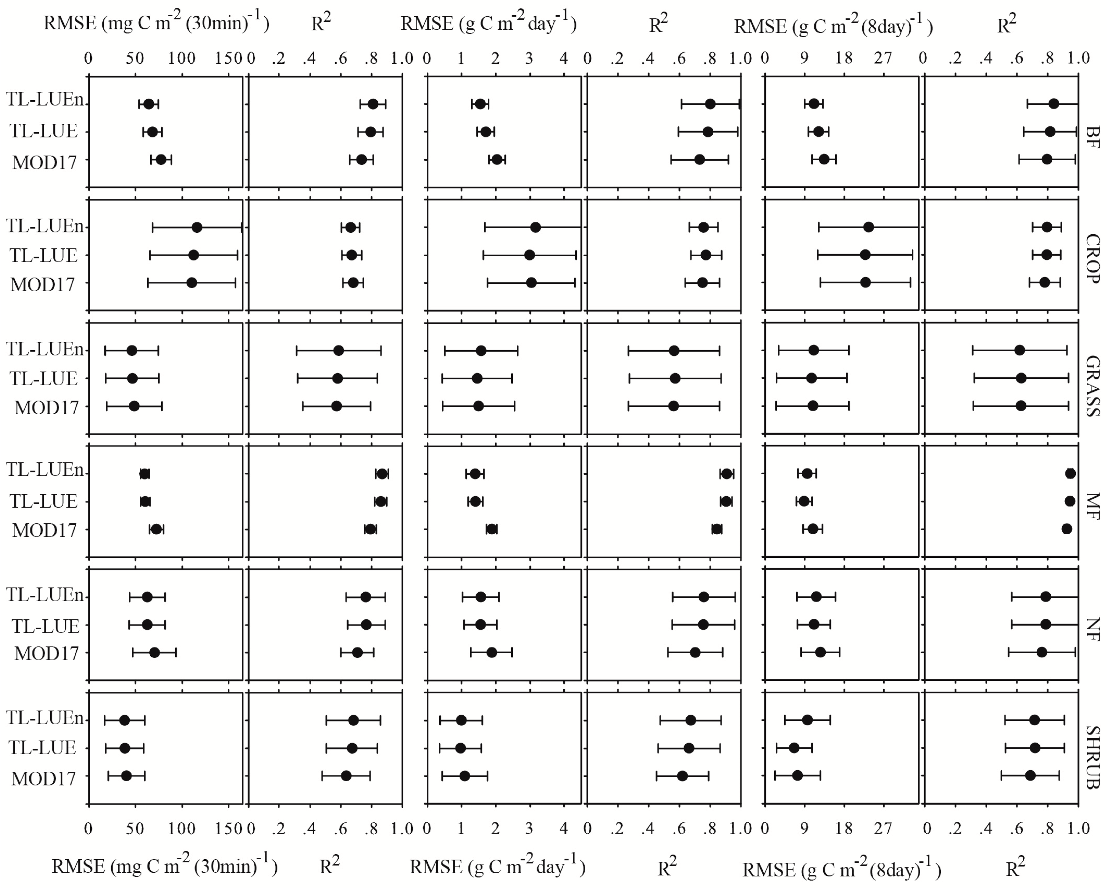
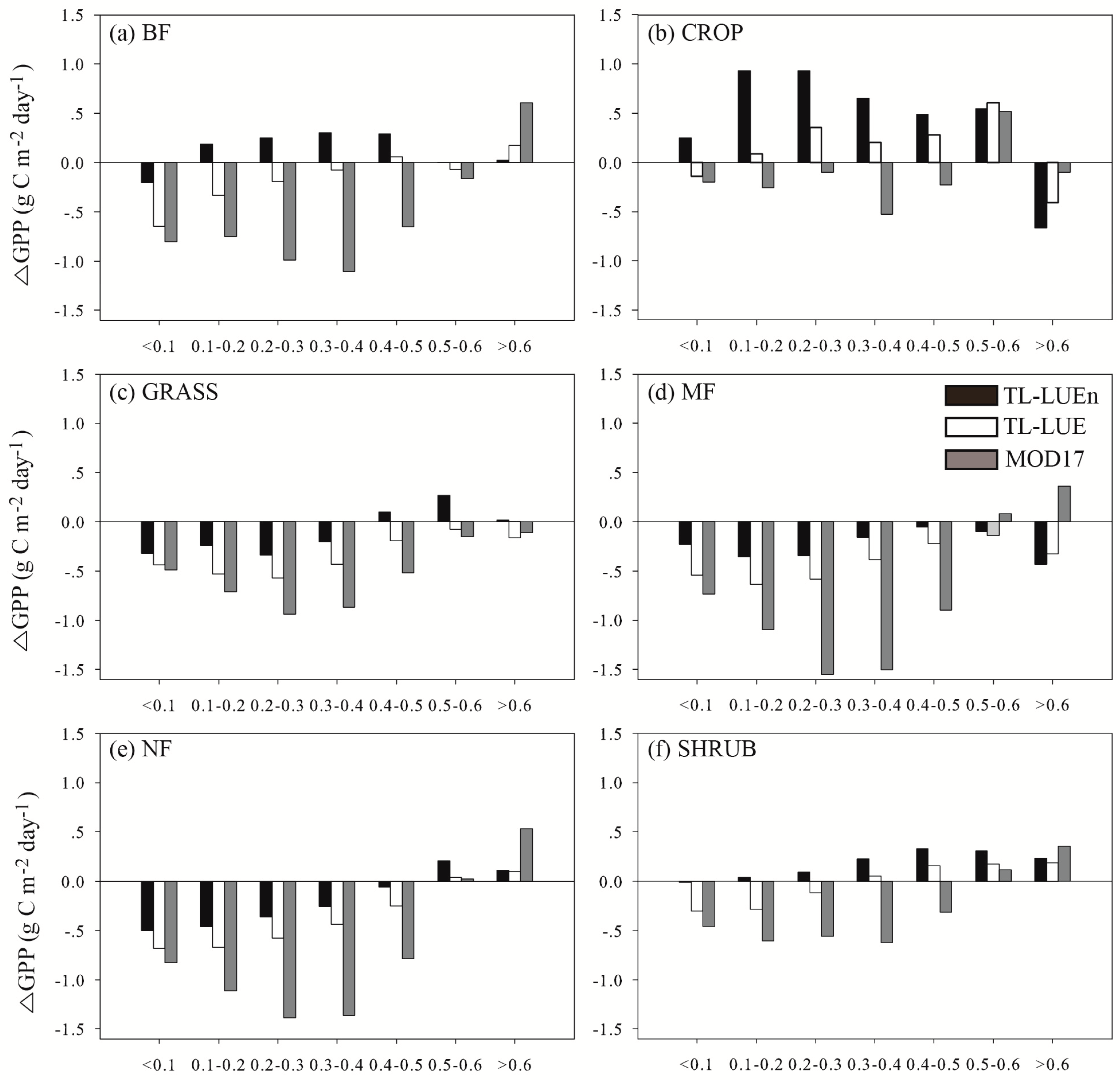
- At the half-hourly temporal scale, TL-LUEn and TL-LUE outperformed MOD17 for all vegetation types but CROP. The outperformance of TL-LUEn and TL-LUE over MOD17 was more distinct for forests than for GRASS and SHRUB vegetation types. With the increase of temporal scales, the improvement of both TL-LUEn and TL-LUE over MOD17 decreased. At the daily temporal scale, both TL-LUEn and TL-LUE performed better than MOD17 for forests and SHRUB. TL-LUE also outperformed MOD17 slightly for other non-forest types (CROP and GRASS). TL-LUEn only performed better than TL-LUE for BF. At the 8-day temporal scale, TL-LUEn only outperformed MOD17 for forests while TL-LUE performed better than MOD17 for all vegetation types. TL-LUEn only slightly outperformed TL-LUE for BF.
- (4)
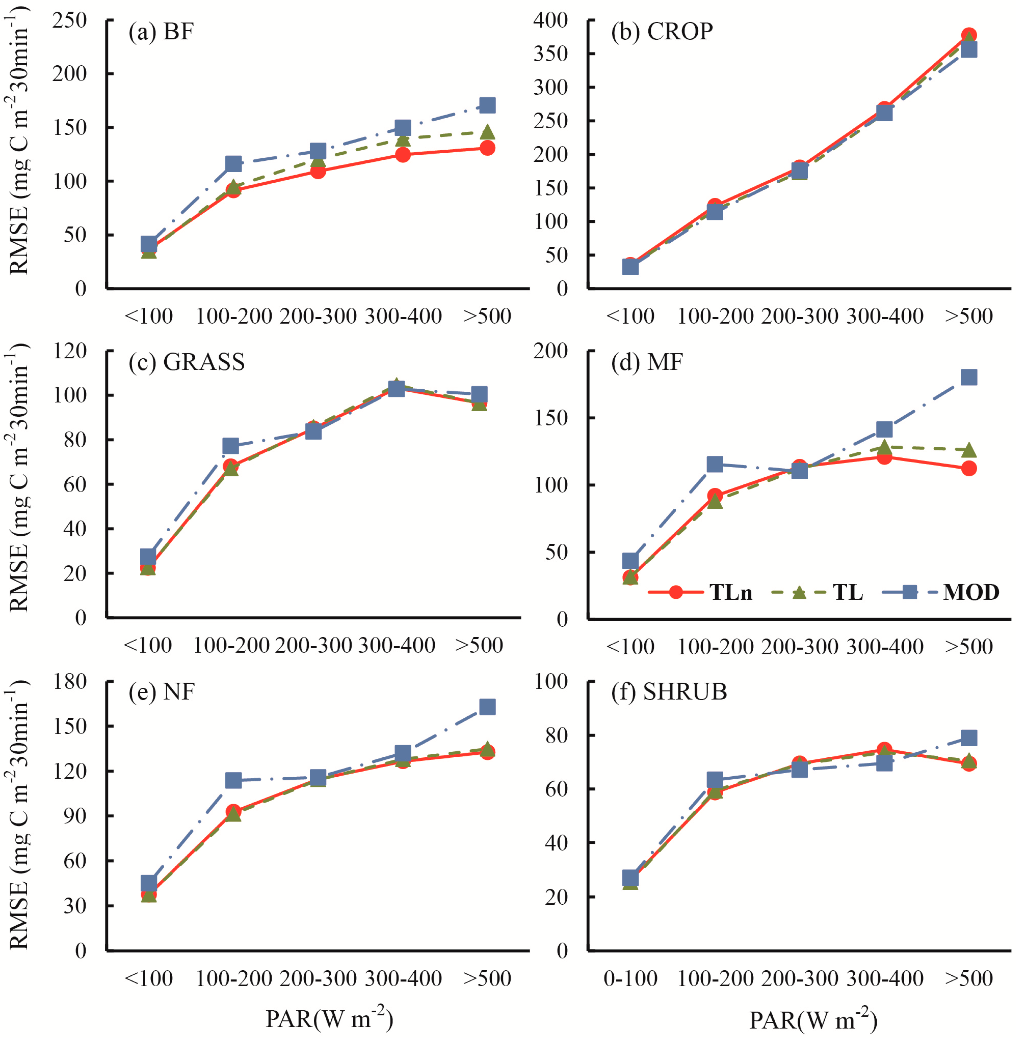
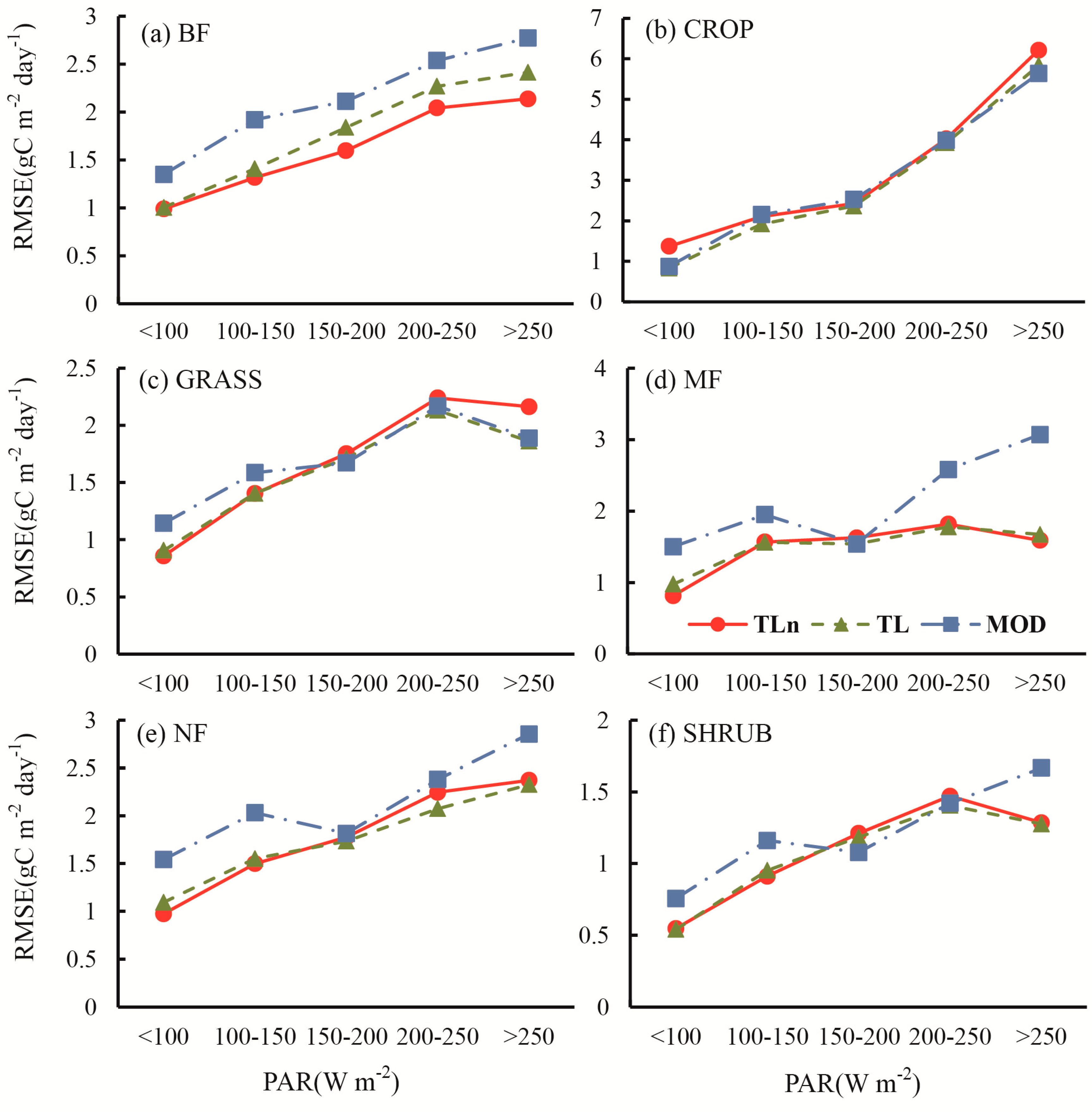
- The improvement of TL-LUEn and TL-LUE over the MOD17 for forests was mainly achieved by the correction of the underestimation of GPP under low incident PAR and the overestimation of GPP under high incident PAR occurring in the MOD17.
- (5)
- TL-LUEn is more applicable at individual sites at the half-hourly scale. TL-LUE could be regionally used at half-hourly, daily and 8-day scales, owing to its excellent performance and small parameter variations at different temporal scales and for most vegetation types. MOD17 is also an applicable option at 8-day scale.
Acknowledgements
Author Contributions
Conflicts of Interest
References
- Le Quéré, C.; Raupach, M.R.; Canadell, J.G.; Marland, G. Trends in the sources and sinks of carbon dioxide. Nature 2009, 2, 831–836. [Google Scholar]
- Beer, C.; Reichstein, M.; Tomelleri, E.; Ciais, P.; Jung, M.; Carvalhais, N.; Rödenbeck, C.; AltafArain, M.; Baldocchi, D.; Bonan, G.B.; et al. Terrestrial gross carbon dioxide uptake: Global distribution and covariation with climate. Science 2010, 329, 834–838. [Google Scholar] [CrossRef] [PubMed]
- Le Quéré, C.; Andres, R.J.; Boden, T.; Conway, T.; Houghton, R.A.; House, J.I.; Marland, G.; Peters, G.P.; van der Werf, G.R.; Ahlstrom, A.; et al. The global carbon budget 1959–2011. Earth Syst. Sci. Data 2013, 5, 165–185. [Google Scholar] [CrossRef] [Green Version]
- Zhang, F.M.; Chen, J.M.; Chen, J.Q.; Gough, C.M.; Martin, T.A.; Dragoni, D. Evaluating spatial and temporal patterns of modis gpp over the conterminous U.S. Against flux measurements and a process model. Remote Sens. Environ. 2012, 124, 717–729. [Google Scholar] [CrossRef]
- Farquhar, G.D.; von Caemmerer, S.; Berry, J.A. A biochemical model of photosynthetic CO2 assimilation in leaves of c3 species. Planta 1980, 149, 78–90. [Google Scholar] [CrossRef] [PubMed]
- Wang, F.M.; Chen, J.M.; Gonsamo, A.; Zhou, B.; Cao, F.F.; Yi, Q.X. A two-leaf rectangular hyperbolic model for estimating GPP across vegetation types and climate conditions. J. Geophys. Res. 2014. [Google Scholar] [CrossRef]
- Potter, C.S.; Randerson, J.T.; Field, C.B.; Matson, P.A.; Vitousek, P.M.; Mooney, H.A.; Klooster, S.A. Terrestrial ecosystem production: A process model based on global satellite and surface data. Glob. Biogeochem.Cy. 1993, 7, 811–841. [Google Scholar] [CrossRef]
- Running, S.W.; Nemani, R.R.; Heinsch, F.A.; Zhao, M.S.; Reeves, M.; Hashimoto, H. A continuous satellite-drived measure of global terrestrial primary production. BioSciense 2004, 54, 547–560. [Google Scholar] [CrossRef]
- Yuan, W.P.; Liu, S.G.; Zhou, G.S.; Zhou, G.Y.; Tieszen, L.L.; Baldocchi, D.; Bernhofer, C.; Gholz, H.; Goldstein, A.H.; Goulden, M.L.; et al. Deriving a light use efficiency model from eddy covariance flux data for predicting daily gross primary production across biomes. Agric. For. Meteorol. 2007, 143, 189–207. [Google Scholar] [CrossRef]
- Xiao, X.M.; Zhang, Q.Y.; Braswell, B.; Urbanski, S.; Boles, S.; Wofsy, S.; Moore, B.; Ojima, D. Modeling gross primary production of temperate deciduous broadleaf forest using satellite images and climate data. Remote Sens. Environ. 2004, 91, 256–270. [Google Scholar] [CrossRef]
- Monteith, J.L. Solar radiation and productivity in tropical ecosystems. J. Appl. Ecol. 1972, 9, 747–766. [Google Scholar] [CrossRef]
- Monteith, J.L.; Moss, C.J. Climate and the efficiency of crop production in britain. Philos. Trans. R. Soc. London, Ser. B. 1977, 281, 277–294. [Google Scholar] [CrossRef]
- Gu, L.H.; Baldocchi, D.; Verma, S.B.; Black, T.A.; Vesala, T.; Falge, E.M.; Dowty, P.R. Advantages of diffuse radiation for terrestrial ecosystem productivity. J. Geophys. Res. 2002. [Google Scholar] [CrossRef]
- Gu, L.H.; Baldocchi, D.D.; Wofsy, S.C.; Munger, J.W.; Michalsky, J.J.; Urbanski, S.P.; Boden, T.A. Response of a deciduous forest to the mount pinatubo eruption: Enhanced photosynthesis. Science 2003, 299, 2035–2038. [Google Scholar] [CrossRef] [PubMed]
- Law, B.E.; Falge, E.; Baldocchi, D.D.; Bakwin, P.; Berbigier, K.; Davis, A.J.; Dolman, M.; Falk, J.D.; Fuentes, A.; Goldstein, A.; et al. Environmental controls over carbon dioxide and water vapor exchange of terrestrial vegetation. Agric. For. Meteorol. 2002, 113, 97–120. [Google Scholar] [CrossRef]
- Roderick, M.L.; Farquhar, G.D.; Berry, S.L.; Noble, I.R. On the direct effect of clouds and atmospheric particles on the productivity and structure of vegetation. Oecologia 2001, 129, 21–30. [Google Scholar] [CrossRef]
- Choudhury, B.J. Estimating gross photosynthesis using satellite and ancillary data: Approach and preliminary results. Remote Sens. Environ. 2001, 75, 1–21. [Google Scholar] [CrossRef]
- Alton, P.B.; North, P.R.; Los, S.O. The impact of diffuse sunlight on canopy light-use efficiency, gross photosynthetic product and net ecosystem exchange in three forest biomes. Glob. Change Biol. 2007, 2007, 776–787. [Google Scholar] [CrossRef]
- Alton, P.B. Reduced carbon sequestration in terrestrial ecosystems under overcast skies compared to clear skies. Agric. For. Meteorol. 2008, 148, 1641–1653. [Google Scholar] [CrossRef]
- Cai, T.; Black, T.A.; Jassal, R.S.; Morgenstern, K.; Nesic, Z. Incorporating diffuse photosynthetically active radiation in a single-leaf model of canopy photosynthesis for a 56-year-old douglas-fir forest. Int. J. Biometeorol. 2009, 53, 135–148. [Google Scholar] [CrossRef] [PubMed]
- Zhang, M.; Yu, G.R.; Zhuang, J.; Gentry, R.; Fu, Y.L.; Sun, X.M.; Zhang, L.M.; Wen, X.F.; Wang, Q.F.; Han, S.J.; et al. Effects of cloudiness change on net ecosystem exchange, light use efficiency, and water use efficiency in typical ecosystems of china. Agric. For. Meteorol. 2011, 151, 803–816. [Google Scholar] [CrossRef]
- Propastin, P.; Ibrom, A.; Knohl, A.; Erasmi, S. Effects of canopy photosynthesis saturation on the estimation of gross primary productivity from modis data in a tropical forest. Remote Sens. Environ. 2012, 121, 252–260. [Google Scholar] [CrossRef]
- He, M.Z.; Ju, W.M.; Zhou, Y.L.; Chen, J.M.; He, H.L.; Wang, S.Q.; Wang, H.M.; Guan, D.X.; Yan, J.H.; Hao, Y.B.; et al. Development of a two-leaf light use efficiency model for improving the calculation of terrestrial gross primary production. Agric. For. Meteorol. 2013, 173, 28–39. [Google Scholar] [CrossRef]
- Chen, J.M.; Liu, J.; Cihlar, J.; Goulden, M.L. Daily canopy photosynthesis model through temporal and spatial scaling for remote sensing applications. Ecol. Model. 1999, 124, 99–119. [Google Scholar] [CrossRef]
- DePury, D.G.G.; Farquhar, G.D. Simple scaling of photosynthesis from leaves to canopies without the errors of big-leaf models. Plant Cell Environ. 1997, 20, 537–557. [Google Scholar] [CrossRef]
- Wang, Y.P.; Leuning, R. A two-leaf model for canopy conductance, photosynthesis and partitioning of available energy I: Model description and comparison with a multi-layered model. Agric. For. Meteorol. 1998, 91, 89–111. [Google Scholar] [CrossRef]
- Falge, E.; Baldocchi, D.; Olson, R.; Anthoni, P.; Aubinet, M.; Bernhofer, C.; Burba, G.; Ceulemans, R.; Clement, R.; Dolman, H.; et al. Gap filling strategies for defensible annual sums of net ecosystem exchange. Agric. For. Meteorol. 2001, 107, 43–69. [Google Scholar] [CrossRef]
- Turner, D.P.; Urbanski, S.; Bremer, D.; Wofsy, S.C.; Meyers, T.; Gower, S.T.; Gregory, M. A cross-biome comparison of daily light use efficiency for gross primary production. Glob. Change Biol. 2003, 9, 383–395. [Google Scholar] [CrossRef]
- Gao, Y.N.; Yu, G.R.; Yan, H.M.; Zhu, X.J.; Li, S.G.; Wang, Q.F.; Zhuang, J.H.; Wang, Y.F.; Li, Y.N.; Zhao, L.M.; et al. A modis-based photosynthetic capacity model to estimate gross primary production in northern China and the tibetan plateau. Remote Sens. Environ. 2014, 148, 108–118. [Google Scholar] [CrossRef]
- Lasslop, G.; Reichstein, M.; Papale, D.; Richardson, A.D.; Arneth, A.; Barr, A.; Stoy, P.; Wohlfahrt, G. Separation of net ecosystem exchange into assimilation and respiration using a light response curve approach: Critical issues and global evaluation. Glob. Change Biol. 2010, 16, 187–208. [Google Scholar] [CrossRef]
- Thanyapraneedkul, J.; Muramatsu, K.; Daigo, M.; Furumi, S.; Soyama, N.; Nasahara, K.N.; Muraoka, H.; Noda, H.M.; Nagai, S.; Maeda, T.; et al. A vegetation index to estimate terrestrial gross primary production capacity for the Global Change Observation Mission-Climate (GCOM-C)/Second-Generation Global Imager (SGLI) satellite sensor. Remote Sens. 2012, 4, 3689–3720. [Google Scholar] [CrossRef]
- Yuan, W.P.; Cai, W.W.; Xia, J.Z.; Chen, J.Q.; Liu, S.G.; Dong, W.J.; Merbold, L.; Law, B.; Arain, A.; Beringer, J.; Bernhofer, C.; Black, A.; Blanken, P.D.; et al. Global comparison of light use efficiency models for simulating terrestrial vegetation gross primary production based on the lathuile database. Remote Sens. Environ. 2014, 192–193, 108–120. [Google Scholar]
- Song, C.H. Optical remote sensing of terrestrial ecosystem primary productivity. Progr. Phys. Geogr. 2013, 37, 834–854. [Google Scholar] [CrossRef]
- Peters, W.; Jacobson, A.R.; Sweeney, C.; Andrews, A.E.; Conway, T.J.; Masarie, K.; Miller, J.B.; Bruhwiler, L.M.P.; Pétron, G.; Hirsch, A.I.; et al. An atmospheric perspective on north american carbon dioxide exchange: Carbontracker. Proc. Natl. Acad. Sci. USA 2007, 104, 18925–18930. [Google Scholar] [CrossRef] [PubMed]
- Fluxdata.org. Available online: http://www.fluxdata.org/default.aspx (accessed on 10 Decmber 2013).
- Baldocchi, D.D.; Falge, E.; Gu, L.H.; Olson, R.; Hollinger, D.; Running, S. W.; Anthoni, P.; Bernhofer, Ch.; Davis, K.; Evans, R.; et al. Fluxnet: A new tool to study the temporal and spatial variability of ecosystem-scale carbon dioxide, water vapor, and energy flux densities. Bull. Am. Meteorol. Soc. 2001, 82, 2415–2434. [Google Scholar] [CrossRef]
- Baldocchi, D.D. Breathing of the terrestrial biosphere: Lessons learned from a global network of carbon dioxide flux measurement systems. Aust. J. Bot. 2008, 56, 1–26. [Google Scholar] [CrossRef]
- Papale, D.; Valentini, A. A new assessment of european forests carbon exchange by eddy fluxes and artificial neural network spatialization. Glob. Change Biol. 2003, 9, 525–535. [Google Scholar] [CrossRef]
- Reichstein, M.; Falge, E.; Baldocchi, D.; Papale, D.; Aubinet, M.; Berbigier, P.; Bernhofer, C.; Buchmann, N.; Gilmanov, T.; Granier, A.; et al. On the separation of net ecosystem exchange into assimilation and ecosystem respiration: Review and improved algorithm. Glob. Change Biol. 2005, 11, 1424–1439. [Google Scholar] [CrossRef]
- Papale, D.; Reichstein, M.; Aubinet, M.; Canfora, E.; Bernhofer, C.; Kutsch, W.; Longdoz, B.; Rambal, S.; Valentini, R.; Vesala, T.; et al. Towards a standardized processing of net ecosystem exchange measured with eddy covariance technique: Algorithms and uncertainty estimation. Biogeosciences 2006, 3, 571–583. [Google Scholar] [CrossRef]
- Moffat, A.M.; Papale, D.; Reichstein, M.; Hollinger, D.Y.; Richardson, A.D.; Barr, A.G.; Beckstein, C.; Braswell, B.H.; Churkina, G.; Desai, A.R.; et al. Comprehensive comparison of gap-filling techniques for eddy covariance net carbon fluxes. Agric. For. Meteorol. 2007, 147, 209–232. [Google Scholar] [CrossRef]
- Gholz, H.L.; Clark, K.L. Energy exchange across a chronose-quence of slash pine forests in florida. Agric. For. Meteorol. 2002, 112, 87–102. [Google Scholar] [CrossRef]
- Fischer, M.L.; Billesbach, D.P.; Riley, W.J.; Berry, J.A.; Torn, M.S. Spatiotemporal variations in growing season exchanges of CO2, H2O, and sensible heat in agricultural fields of the southern great plains. Earth Interact. 2007, 11, 1–21. [Google Scholar] [CrossRef]
- Wilson, T.B.; Meyers, T.P. Determining vegetation indices from solar and photosynthetically active radiation fluxes. Agric. For. Meteorol. 2007, 144, 160–179. [Google Scholar] [CrossRef]
- Humphreys, E.R.; Black, T.A.; Morgenstern, K.; Cai, T.; Drewitt, G.B.; Nesic, Z.; Trofymow, J.A. Carbon dioxide fluxes in coastal douglas-fir stands at different stages of development after clearcut harvesting. Agric. For. Meteorol. 2006, 140, 6–22. [Google Scholar] [CrossRef]
- Jenkins, J.P.; Richardson, A.D.; Braswell, B.H.; Ollinger, S.V.; Hollinger, D.Y.; Smith, M.L. Refining light-use efficiency calculations for a deciduous forest canopy using simultaneous tower-based carbon flux and radiometric measurements. Agric. For. Meteorol. 2007, 143, 64–79. [Google Scholar] [CrossRef]
- Zhang, J.H.; Han, S.J.; Yu, G.R. Seasonal variation in carbon dioxide exchange over a 200-year-old chinese broad-leaved korean pine mixed forest. Agric. For. Meteorol. 2006a, 137, 150–165. [Google Scholar] [CrossRef]
- Zhang, J.H.; Yu, G.R.; Han, S.J.; Guan, D.X.; Sun, X.M. Seasonal and annual variation of CO2 flux above a broad-leaved korean pine mixed forest. Sci. China Series D: Earth Scie. 2006b, 49, 63–73. [Google Scholar]
- Zhang, L.; Luo, Y.Q.; Yu, G.R.; Zhang, L.M. Estimated carbon residence times in three forest ecosystems of eastern China: Applications of probabilistic inversion. J. Geophys. Res. 2000. [Google Scholar] [CrossRef]
- Reichstein, M.; Ciais, P.; Papale, D.; Valentini, R.; Running, S.; Vivoy, N.; Cramer, W.; Granier, A.; Ogée, J.; Allard, V.; et al. Reduction of ecosystem productivity and respiration during the european summer 2003 climate anomaly: A joint flux tower, remote sensing and modelling analysis. Glob. Change Biol. 2006, 13, 634–651. [Google Scholar] [CrossRef]
- Milyukova, I.M.; Kolle, O.; Varlagin, A.V.; Vygodskaya, N.N.; Schulze, E.D.; Lloyd, J. Carbon balance of a southern taiga spruce stand in european russia. Tellus B 2002, 54, 429–442. [Google Scholar] [CrossRef]
- Mund, M.; Kutsch, W.; Wirth, C.; Kahl, T.; Knohl, A.; Skomarkova, M.; Schulze, E. The influence of climate and fructification on the inter-annual variability of stem growth and net primary productivity in an old-growth, mixed beech forest. Tree Physiol. 2010, 30, 689–704. [Google Scholar] [CrossRef] [PubMed]
- Urbanski, S.; Barford, C.; Kucharik, C.; Pyle, E.; Budney, J.; McKain, K.; Fitzjarrald, D.; Czikowsky, M.; Munger, J.W. Factors controlling CO2 exchange on timescale from hourly to decadal at harward forest. J. Geophys. Res. 2007. [Google Scholar] [CrossRef]
- Granier, A.; Pilegaard, K.; Jensen, N.O. Similar net ecosystem exchange of beech stands located in france and denmark. Agric. For. Meteorol. 2002, 114, 75–82. [Google Scholar] [CrossRef]
- Hollinger, D.Y.; Goltz, S.M.; Davidson, E.A.; Lee, J.T.; Tu, K.; Valentine, H.T. Seasonal patterns and environmental control of carbon dioxide and water vapour exchange in an ecotonal boreal forest. Glob. Change Biol. 1999, 5, 891–902. [Google Scholar] [CrossRef]
- Hollinger, D.Y.; Aber, J.; Dail, B.; Davidson, E.A.; Goltz, S.M.; Hughes, H.; Leclerc, M.Y.; Lee, J.T.; Richardson, A.D.; Rodrigues, C.; et al. Spatial and temporal variability in forest-atmosphere CO2 exchange. Glob. Change Biol. 2004, 10, 1689–1706. [Google Scholar] [CrossRef]
- Kramer, K.; Leinonen, I.; Bartelink, H.H.; Berbigier, P.; Borghetti, M.; Bernhofer, C.; Cienciala, E.; Dolman, A.J.; Froer, O.; Gracia, C.A.; et al. Evaluation of six process-based forest growth models using eddy-covariance measurements of CO2 and H2O fluxes at six forest sites in europe. Glob. Change Biol. 2002, 8, 213–230. [Google Scholar] [CrossRef]
- Scott, R.L. Using watershed water balance to evaluate the accuracy of eddy covariance evaporation measurements for three semiarid ecosystems. Agric. For. Meteorol. 2010, 150, 219–225. [Google Scholar] [CrossRef]
- Powell, T.; Bracho, R.; Li, J.; Dore, S.; Hinkle, C.; Drake, B. Environmental controls over net ecosystem carbon exchange of scrub oak in central florida. Agric. For. Meteorol. 2006, 141, 19–34. [Google Scholar] [CrossRef]
- Dolman, A.J.; Moors, E.J.; Elbers, J.A. The carbon uptake of amid latitude pine forest growing on sandy soil. Agric. For. Meteorol. 2002, 111, 157–170. [Google Scholar] [CrossRef]
- Verma, S.B.; Dobermann, A.; Cassman, K.G.; Walters, D.T.; Knops, J.M.; Arkebauer, T.J.; Suyker, A.E.; Burba, G.G.; Amos, B.; Yang, H.; et al. Annual carbon dioxide exchange in irrigated and rainfed maize-based agroecosystems. Agric. For. Meteorol. 2005, 131, 77–96. [Google Scholar] [CrossRef]
- Law, B.E.; Sun, O.; Campbell, J.; Van Tuyl, S.; Thornton, P. Changes in carbon storage and fluxes in a chronosequence of ponderosa pine. Glob. Change Biol. 2003, 9, 510–524. [Google Scholar] [CrossRef]
- Thomas, C.K.; Law, B.E.; Irvine, J.; Martin, J.G.; Pettijohn, J.C.; Davis, K.J. Seasonal hydrology explains interannual and seasonal variation in carbon and water exchange in a semi-arid mature ponderosa pine forest in central oregon. J Geophys. Res. 2009, 114, G04006. [Google Scholar]
- Bracho, R.G.; Starr, G.; Gholz, H.; Martin, T.A.; Cropper, J.W.P.; Loescher, H.W. Controls on carbon dynamics by ecosystem structure and climate for southeastern us slash pine plantations. Ecol. Monogr. 2012, 82, 101–128. [Google Scholar] [CrossRef]
- Schmid, H.; Grimmond, C.; Cropley, F.; Offerle, B.; Su, H. Measurements of CO2 and energy fluxes over a mixed hardwood forest in the mid-western united states. Agric. For. Meteorol. 2000, 103, 357–374. [Google Scholar] [CrossRef]
- Ruehr, N.K.; Martin, J.; Law, B.E. Effects of water availability on carbon and water exchange in a young ponderosa pine forest: Above- and belowground responses. Agric. For. Meteorol. 2012, 164, 136–148. [Google Scholar] [CrossRef]
- Vickers, D.; Thomas, C.K.; Pettijohn, C.; Martin, J.G.; Law, B.E. Five years of carbon fluxes and inherent water-use efficiency at two semi-arid pine forests with different disturbance histories. Tellus B 2012, 64, 17159. [Google Scholar] [CrossRef]
- Gu, L.H.; Meyers, T.; Pallardy, S.G.; Hanson, P.J.; Yang, B.; Heuer, M.; Hosman, K.P.; Riggs, J.S.; Sluss, D.; Wullschleger, S.D. Direct and indirect effects of atmospheric conditions and soil moisture on surface energy partitioning revealed by a prolonged drought at a temperate forest site. J. Geophys. Res. 2006. [Google Scholar] [CrossRef]
- Noormets, A.; Gavazzi, M.J.; McNulty, S.G.; Domec, J.C.; Sun, G.; King, J.; Chen, J. Response of carbon fluxes to drought in a coastal plain loblolly pine forest. Glob. Change Biol. 2009, 16, 272–287. [Google Scholar] [CrossRef]
- Wohlfahrt, G.; Hammerle, A.; Haslwanter, A.; Bahn, M.; Tappeiner, U.; Cernusca, A. Seasonal and inter-annual variability of the net ecosystem CO2 exchange of a temperate mountain grassland: Effects of weather and management. J. Geophys. Res. 2008. [Google Scholar] [CrossRef]
- Monson, R.K.; Turnipseed, A.A.; Sparks, J.P.; Harley, P.C.; Scott Denton, L.E.; Sparks, K.; Huxman, T.E. Carbon sequestration in a high-elevation, subalpine forest. Glob. Change Biol. 2002, 8, 459–478. [Google Scholar] [CrossRef]
- Lafleur, P.; Roulet, N.; Bubier, J.; Frolking, S.; Moore, T. Interannual variability in the peatland-atmosphere carbon dioxide exchange at an ombrotrophic bog. Glob. Biogeochem.Cy. 2003. [Google Scholar] [CrossRef]
- Allard, V.; Ourcival, J. M.; Rambal, S.; Joffre, R.; Rocheteau, A. Seasonal and annual variation of carbon exchange in an evergreen mediterranean forest in southern france. Glob. Change Biol. 2008, 14, 714–725. [Google Scholar] [CrossRef]
- Bergeron, O.; Margolis, H.; Black, T.; Coursolle, C.; Dunn, A.; Barr, A.; Wofsy, S. Comparison of carbon dioxide fluxes over three boreal black spruce forests in canada. Glob. Change Biol. 2007, 13, 89–107. [Google Scholar] [CrossRef]
- Yu, G.R.; Wen, X.F.; Sun, X.M.; Tanner, B.D.; Lee, X.H.; Chen, J.Y. Overview of ChinaFlux and evaluation of its eddy covariance measurement. Agric. For. Meteorol. 2006, 137, 125–137. [Google Scholar] [CrossRef]
- Montagnani, L.; Manca, G.; Canepa, E.; Georgieva, E.; Acosta, M.; Feigenwinter, C.; Janous, D.; Kerschbaumer, G.; Lindroth, A.; Minach, L.; et al. A new mass conservation approach to the study of CO2 advection in an alpine forest. J. Geophys. Res. 2009. [Google Scholar] [CrossRef]
- Griffis, T.J.; Sargent, S.D.; Baker, J.M.; Lee, X.; Tanner, B.D.; Greene, J.; Swiatek, E.; Billmark, K. Direct measurement of biosphere-atmosphere isotopic CO2 exchange using the eddy covariance technique. J. Geophys. Res. 2008. [Google Scholar] [CrossRef]
- Bavin, T.K.; Griffis, T.J.; Baker, J.M.; Venterea, R.T. Impacts of reduced tillage and cover cropping on the greenhouse gas budget of a maize/soybean rotation ecosystem. Agr. Ecosyst. Environ. 2009, 134, 234–242. [Google Scholar] [CrossRef]
- Keenan, T.; Garcia, R.; Friend, A. D.; Zaehle, S.; Gracia, C.; Sabate, S. Improved understanding of drought controls on seasonal variation in mediterranean forest canopy CO2 and water fluxes through combined in situ measurements and ecosystem modeling. Biogeosciences 2009, 6, 1423–1444. [Google Scholar] [CrossRef] [Green Version]
- Luo, H.; Oechel, W.; Hastings, S.; Zulueta, R.; Qian, Y.; Kwon, H. Mature semiarid chaparral ecosystems can be a significant sink for atmospheric carbon dioxide. Glob. Change Biol. 2007, 13, 386–396. [Google Scholar] [CrossRef]
- Pilegaard, K.; Hummelshoj, P.; Jensen, N.O.; Chen, Z. Two years of continuous co2 eddy-flux measurements over a danish beech forest. Agric. For. Meteorol. 2001, 107, 29–41. [Google Scholar] [CrossRef]
- Migliavacca, M.; Reichstein, M.; Richardson, A.D.; Colombo, R.; Sutton, M.A.; Lasslop, G.; Tomelleri, E.; Wohlfahrt, G.; Carvalhais, N.; Cescatti, A. Semiempirical modeling of abiotic and biotic factors controlling ecosystem respiration across eddy covariance sites. Glob. Change Biol. 2011, 17, 390–409. [Google Scholar] [CrossRef] [Green Version]
- Grünwald, T.; Bernhofer, C. A decade of carbon, water and energy flux measurements of an old spruce forest at the anchor station tharandt. Tellus B 2007, 59, 387–396. [Google Scholar] [CrossRef]
- Hirano, T.; Hirata, R.; Fujinuma, Y.; Saigusa, N.; Yamamoto, S.; Harazono, Y.; Takada, M.; Inukai, K.; Inoue, G. Co2 and water vapor exchange of a larch forest in northern japan. Tellus B 2003, 55, 244–257. [Google Scholar] [CrossRef]
- Baldocchi, D.D.; Xu, L.K.; Kiang, N. How plant functional type, weather, seasonal drought, and soil physical properties alter water and energy fluxes of an oak-grass savanna and an annualgrassland. Agric. For. Meteorol. 2004, 123, 13–39. [Google Scholar] [CrossRef]
- Goulden, M.L.; McMillan, A.M.S.; Winston, G.C.; Rocha, A.V.; Manies, K.L.; Harden, J.W.; Bond-Lamberty, B.P. Patterns of NPP, GPP, respiration, and nep during boreal forest succession. Glob. Change Biol. 2011, 17, 855–871. [Google Scholar] [CrossRef]
- Curtis, P.S.; Vogel, C.S.; Gough, C.M.; Schmid, H.P.; Su, H.B.; Bovard, B.D. Respiratory carbon losses and the carbon use efficiency of a northern hardwood forest, 1999–2003. New Phytol. 2005, 167, 437–456. [Google Scholar] [CrossRef] [PubMed]
- Aubinet, M.; Chermanne, B.; Vandenhaute, M.; Longdoz, B.; Yernaux, M.; Laitat, E. Long term carbon dioxide exchange above a mixed forest in the belgian ardennes. Agric. For. Meteorol. 2001, 108, 293–315. [Google Scholar] [CrossRef]
- Bolstad, P.V.; Davis, K.J.; Martin, J.; Cook, B.D.; Wang, W. Component and whole-system respiration fluxes in northern deciduous forests. Tree Physiol. 2004, 24, 493–504. [Google Scholar] [CrossRef] [PubMed]
- Rebmann, C.; Zeri, M.; Lasslop, G.; Mund, M.; Kolle, O.; Schulze, E.; Feigenwinter, C. Treatment and assessment of the co2-exchange at a complex forest site in thuringia, germany. Agric. For. Meteorol. 2009, 150, 684–691. [Google Scholar] [CrossRef]
- Running, S.W.; Thornton, P.E.; Nemani, R.; Glassy, J.M. Global terrestrial gross and net primary productivity from the earth observing system. In Methods in Ecosystem Science; Sala, O.E., Jackson, R.B., Mooney, H.A., Howarth, R.W., Eds.; Springer-Verlag: New York, NY, USA, 2000; pp. 44–57. [Google Scholar]
- Monteith, J.L. The photosynthesis and transpiration of crops. Exp. Agric. 1966, 2, 1–14. [Google Scholar] [CrossRef]
- Michalsky, J.J. The astronomical almanac's algorithm for approximate solar position (1950–2050). Solar Energy 1988, 40, 227–235. [Google Scholar] [CrossRef]
- Tang, S.; Chen, J.M.; Zhu, Q.; Li, X.; Chen, M.; Sun, R.; Zhou, Y.; Deng, F.; Xie, D. LAI inversion algorithm based on directional reflectance kernels. J. Environ. Manage. 2007, 85, 638–648. [Google Scholar] [CrossRef] [PubMed]
- Grant, I.F.; Prata, A.J.; Cechet, R.P. The impact of the diurnal variation of albedo on the remote sensing of the daily mean albedo of grassland. J. Appl. Meteorol. 2000, 39, 231–244. [Google Scholar] [CrossRef]
- Singarayer, J.S.; Ridgwell, A.; Irvine, P. Assessing the benefits of crop albedo bio-geoengineering. Environ. Res. Lett. 2009, 4, 045110. [Google Scholar] [CrossRef]
- Metropolis, N.; Rosenbluth, A.W.; Rosenbluth, M.N.; Teller, A.H. Equation of state calculations by fast computing machines. J. Chem. Phys. 1953, 21, 1087–1092. [Google Scholar] [CrossRef]
- Hastings, W.K. Monte carlo sampling methods using markov chains and their applications. Biometrika 1970, 57, 97–109. [Google Scholar] [CrossRef]
- Ruimy, A.; Jarvis, P.G.; Baldocchi, D.D.; Saugier, B. Co2 fluxes over plant canopies and solar radiation: A review. Adv. Ecol. Res. 1995, 26, 1–51. [Google Scholar]
- Li, A.N.; Bian, J.H.; Lei, G.B.; Huang, C.Q. Estimating the maximal light use efficiency for different vegetation through the casa model combined with time-series remote sensing data and ground measurements. Remote Sens. 2012, 4, 3857–3876. [Google Scholar] [CrossRef]
- Braswell, B.H.; Sacks, W.J.; Linder, E.; Schimel, D.S. Estimating diurnal to annual ecosystem parameters by synthesis of a carbon flux model with eddy covariance net ecosystem exchange observations. Glob. Change Biol. 2005, 11, 335–355. [Google Scholar] [CrossRef]
- Raupach, M.R.; Rayner, P.J.; Barrett, D.J.; Defries, R.S.; Heimann, M.; Ojima, D.S.; Quegan, S.; Schmullius, C.C. Model-data synthesis in terrestrial carbon observation: Methods, data requirements and data uncertainty specifications. Glob. Change Biol. 2005, 11, 378–397. [Google Scholar] [CrossRef]
- Xu, T.; White, L.; Hui, D.F.; Luo, Y.Q. Probabilistic inversion of a terrestrial ecosystem model: Analysis of uncertainty in parameter estimation and model prediction. Glob. Biogeochem. Cy. 2006, 20, GB2007. [Google Scholar] [CrossRef]
- Box, G.E.P.; Hunter, W.G.; Hunter, J.S. Statistics for Experimenters; John Wiley & Sons, Inc.: Hoboken, NJ, USA, 1978. [Google Scholar]
- Gebremichael, M.; Barros, A.P. Evaluation of modis gross primary productivity (GPP) in tropical monsoon regions. Remote Sens. Environ. 2006, 100, 150–166. [Google Scholar] [CrossRef]
- Loucks, D.P.; van Beek, E. Model sensitivity and uncertainty analysis. In Water Resources Systems Planning and Management; UNESCO: Rome, Italy, 2005; pp. 255–290. [Google Scholar]
- Sinclair, T.R.S.T. Soybean radiation-use efficiency as influenced by nonuniform specific leaf nitrogen distribution and diffuse radiation. Crop Sci. 1993, 33, 808–812. [Google Scholar] [CrossRef]
- Hammer, G.L.; Wright, G.C. A theoretical analysis of nitrogen and radiation effects on radiation use efficiency in peanut. Austr. J. Agric. Res. 1994, 45, 575–589. [Google Scholar] [CrossRef]
- Turner, D.P.; Ritts, W.D.; Cohen, W.B.; Gower, S.T.; Running, S.W.; Zhao, M.S.; Costa, M.H.; Kirschbaum, A.A.; Ham, J.M.; Saleska, S.R.; Ahl, D.E. Evaluation of modis NPP and GPP products across multiple biomes. Remote Sens. Environ. 2006, 102, 282–292. [Google Scholar] [CrossRef]
- Garbulsky, M.F.; Peñuelas, J.; Papale, D.; Ardö, J.; Goulden, M.J.; Kiely, G.; Richardson, A.D.; Rotenberg, E.; Veenendaal, E.M.; Filella, I. Patterns and controls of the variability of radiation use efficiency and primary productivity across terrestrial ecosystems. Glob. Ecol. Biogeogr. 2011, 19, 253–267. [Google Scholar] [CrossRef]
- Xiao, J.F.; Zhuang, Q.L.; Law, B.E.; Baldocchi, D.D.; Chen, J.Q.; Richardson, A.D.; Melillo, J.M.; Davis, K.J.; Hollinger, D.Y.; Wharton, S.; et al. Assessing net ecosystem carbon exchange of u. S. Terrestrial ecosystems by integrating eddy covariance flux measurements and satellite observations. Agric. Forest Meteorol. 2011, 151, 60–69. [Google Scholar] [CrossRef]
- Chen, T.; van der Werf, G.R.; Dolman, A.J.; Groenendijk, M. Evaluation of cropland maximum light use efficiency using eddy flux measurements in North America and Europe. Geophys. Res. Lett. 2011, 38, L14707. [Google Scholar]
- Leuning, R.; Kelliher, F. M.; DePury, D.G.G.; Schulze, E.D. Leaf nitrogen, photosynthesis, conductance and transpiration: Scaling from leaves to canopy. Plant Cell Environ. 1995, 18, 1183–1200. [Google Scholar] [CrossRef]
- Hollinger, D.Y.; Kelliher, F.M.; Byers, J.N.; Hunt, J.E.; McSeveny, T.M.; Weir, P.L. Carbon dioxide exchange between an undisturbed old-growth temperate forest and the atmosphere. Ecology 1994, 75, 134–150. [Google Scholar] [CrossRef]
- Leuning, R.; Cleugh, H.A.; Zegelin, S.J.; Hughes, D. Carbon and water fluxes over a temperate eucalyptus forest and a tropical wet/dry savanna in australia: Measurements and comparison with modis remote sensing estimates. Agric. Forest Meteorol. 2005, 129, 151–173. [Google Scholar] [CrossRef]
- Hashimoto, H.; Wang, W.L.; Milesi, C.; Xiong, J.; Ganguly, S.; Zhu, Z.; Nemani, R. Structural uncertainty in model-simulated trends of global gross primary production. Remote Sens. 2013, 5, 1258–1273. [Google Scholar] [CrossRef]
- Law, B.E.; Waring, R.H. Combining remote sensing and climatic data to estimate net primary production across oregon. Ecol. Appl. 1994, 4, 717–728. [Google Scholar] [CrossRef]
- Heinsch, F.A.; Zhao, M.S.; Running, S.W.; Kimball, J.S.; Nemani, R.R.; Davis, K.J.; Bolstad, P.V.; Cook, B.D.; Desai, A.R.; Ricciuto, D.M.; et al. Evaluation of remote sensing based terrestrial productivity from modis using regional tower eddy flux network observations. IEEE Trans. Geosci. Remote Sens. 2006, 44, 1908–1925. [Google Scholar] [CrossRef]
- Ide, R.; Nakaji, T.; Oguma, H. Assessment of canopy photosynthetic capacity and estimation of GPP by using spectral vegetation indices and the light–response function in a larch forest. Agric. For. Meteorol. 2010, 150, 389–398. [Google Scholar] [CrossRef]
- Polley, H.W.; Emmerich, W.; Bradford, J.A.; Sims, P.L.; Johnson, D.A.; Saliendra, N.Z.; Svejcar, T.; Angell, R.; Frank, A.B.; Phillips, R.L.; et al. Physiological and environmental regulation of interannual variability in co2 exchange on rangelands in the western united states. Glob. Change Biol. 2010, 16, 990–1002. [Google Scholar] [CrossRef]
- Chen, J.; Zhang, H.; Liu, Z.; Che, M.; Chen, B. Evaluating parameter adjustment in the modis gross primary production algorithm based on eddy covariance tower measurements. Remote Sens. 2014, 6, 3321–3348. [Google Scholar] [CrossRef]
- Cescatti, A.; Marcolla, B.; Vannan, S.K.S.; Pan, J.Y.; Roman, M.O.; Yang, X.Y.; Ciais, P.; Cook, R.B.; Law, B.E.; Matteucci, G.; et al. Intercomparison of modis albedo retrievals and in situ measurements across the global fluxnet network. Remote Sens. Environ. 2012, 121, 323–334. [Google Scholar] [CrossRef]
Appendix

| ID | RMSE (mg C m −2 (30min)−1) | R2 | ||||||
|---|---|---|---|---|---|---|---|---|
| TL-LUEn | TL-LUE | MOD17 | TL-LUEn | TL-LUE | MOD17 | |||
| BF | BEP | 63.381 | 66.958 | 76.423 | 0.819 | 0.783 | 0.689 | |
| DHS | 60.435 | 63.478 | 71.283 | 0.724 | 0.703 | 0.633 | ||
| HA | 59.667 | 64.036 | 71.053 | 0.910 | 0.888 | 0.807 | ||
| HAF | 71.021 | 72.580 | 85.082 | 0.862 | 0.853 | 0.801 | ||
| HES | 76.049 | 85.382 | 99.336 | 0.807 | 0.774 | 0.671 | ||
| MMS | 73.369 | 75.175 | 82.751 | 0.770 | 0.759 | 0.709 | ||
| MOZ | 68.622 | 68.328 | 73.618 | 0.770 | 0.758 | 0.711 | ||
| PUE | 49.406 | 49.861 | 54.236 | 0.806 | 0.801 | 0.770 | ||
| ROC | 79.484 | 80.577 | 84.508 | 0.636 | 0.640 | 0.635 | ||
| UMBS | 49.415 | 66.195 | 79.444 | 0.900 | 0.895 | 0.851 | ||
| WCR | 56.459 | 59.721 | 75.943 | 0.899 | 0.887 | 0.822 | ||
| Average RMSE | 64.301 | 68.390 | 77.607 | Average R2 | 0.809 | 0.795 | 0.736 | |
| CROP | ASM | 48.448 | 50.368 | 46.187 | 0.599 | 0.578 | 0.642 | |
| BON | 112.395 | 108.419 | 102.831 | 0.639 | 0.650 | 0.635 | ||
| MEI | 142.000 | 139.843 | 134.365 | 0.678 | 0.687 | 0.711 | ||
| MER | 161.440 | 158.377 | 158.585 | 0.688 | 0.700 | 0.728 | ||
| MIR | 178.555 | 175.665 | 174.733 | 0.724 | 0.736 | 0.771 | ||
| RG19 | 70.821 | 69.495 | 72.853 | 0.737 | 0.744 | 0.709 | ||
| RG21 | 99.387 | 85.314 | 83.437 | 0.582 | 0.600 | 0.579 | ||
| Average RMSE | 116.149 | 112.497 | 110.427 | Average R2 | 0.664 | 0.671 | 0.682 | |
| GRASS | AUD | 21.885 | 21.481 | 22.053 | 0.200 | 0.212 | 0.276 | |
| FPE | 34.699 | 34.544 | 35.134 | 0.541 | 0.531 | 0.496 | ||
| GCR | 55.747 | 56.305 | 58.141 | 0.831 | 0.823 | 0.815 | ||
| HB | 11.792 | 14.484 | 17.945 | 0.906 | 0.853 | 0.795 | ||
| KED | 33.405 | 33.165 | 32.512 | 0.498 | 0.502 | 0.518 | ||
| NEU | 80.230 | 81.569 | 93.599 | 0.821 | 0.821 | 0.767 | ||
| VRA | 85.744 | 84.997 | 82.802 | 0.310 | 0.315 | 0.352 | ||
| Average RMSE | 46.215 | 46.649 | 48.884 | Average R2 | 0.587 | 0.580 | 0.574 | |
| MF | CBS | 65.447 | 67.410 | 78.617 | 0.819 | 0.813 | 0.750 | |
| HOF | 55.397 | 58.873 | 70.669 | 0.881 | 0.862 | 0.776 | ||
| SOR | 62.126 | 60.641 | 78.508 | 0.915 | 0.909 | 0.832 | ||
| VSA | 56.961 | 55.160 | 62.589 | 0.861 | 0.862 | 0.819 | ||
| Average RMSE | 59.983 | 60.521 | 72.596 | Average R2 | 0.813 | 0.805 | 0.750 | |
| NF | ACA | 77.015 | 76.300 | 75.549 | 0.413 | 0.413 | 0.402 | |
| BD49 | 74.576 | 78.571 | 106.579 | 0.847 | 0.834 | 0.720 | ||
| DH00 | 56.199 | 63.847 | 63.684 | 0.605 | 0.602 | 0.561 | ||
| DH88 | 50.135 | 52.940 | 76.208 | 0.881 | 0.877 | 0.782 | ||
| DON | 87.427 | 87.770 | 84.239 | 0.682 | 0.680 | 0.685 | ||
| ES | 64.787 | 57.208 | 60.443 | 0.770 | 0.769 | 0.726 | ||
| FY | 65.602 | 61.214 | 67.128 | 0.844 | 0.855 | 0.770 | ||
| HY | 31.505 | 30.950 | 38.836 | 0.951 | 0.947 | 0.885 | ||
| LOB | 75.394 | 73.753 | 80.112 | 0.782 | 0.781 | 0.739 | ||
| MIN | 62.065 | 59.961 | 64.929 | 0.826 | 0.828 | 0.788 | ||
| MNY | 42.416 | 45.296 | 44.548 | 0.738 | 0.721 | 0.663 | ||
| NCL | 93.203 | 91.163 | 116.335 | 0.838 | 0.842 | 0.793 | ||
| NR | 38.822 | 36.581 | 43.257 | 0.792 | 0.805 | 0.739 | ||
| QMB | 26.751 | 25.044 | 29.041 | 0.633 | 0.673 | 0.597 | ||
| QYZ | 78.560 | 78.520 | 80.415 | 0.756 | 0.758 | 0.747 | ||
| REN | 77.531 | 79.238 | 79.692 | 0.663 | 0.657 | 0.617 | ||
| SRO | 81.280 | 78.843 | 77.470 | 0.725 | 0.719 | 0.682 | ||
| THA | 67.968 | 68.762 | 76.497 | 0.850 | 0.848 | 0.765 | ||
| TMK | 59.161 | 64.370 | 105.229 | 0.935 | 0.919 | 0.799 | ||
| U50 | 34.898 | 30.674 | 36.441 | 0.633 | 0.710 | 0.606 | ||
| WET | 70.679 | 72.746 | 75.443 | 0.862 | 0.862 | 0.803 | ||
| Average RMSE | 62.665 | 62.560 | 70.575 | Average R2 | 0.763 | 0.767 | 0.708 | |
| SHRUB | KEN | 59.876 | 58.965 | 62.697 | 0.811 | 0.811 | 0.789 | |
| MIZ | 73.406 | 73.674 | 73.614 | 0.840 | 0.844 | 0.831 | ||
| OEM | 16.690 | 19.447 | 23.973 | 0.818 | 0.785 | 0.713 | ||
| SON | 28.248 | 29.451 | 25.293 | 0.381 | 0.400 | 0.391 | ||
| SRM | 30.431 | 29.824 | 30.056 | 0.450 | 0.457 | 0.462 | ||
| TRA | 55.896 | 52.920 | 51.908 | 0.639 | 0.663 | 0.680 | ||
| U89 | 23.456 | 21.613 | 27.365 | 0.779 | 0.781 | 0.679 | ||
| U98 | 20.229 | 23.686 | 27.612 | 0.746 | 0.648 | 0.543 | ||
| Average RMSE | 38.529 | 38.698 | 40.315 | Average R2 | 0.683 | 0.674 | 0.636 | |
| ID | RMSE (g C m −2 day −1) | R2 | ||||||
|---|---|---|---|---|---|---|---|---|
| TL-LUEn | TL-LUE | MOD17 | TL-LUEn | TL-LUE | MOD17 | |||
| BF | BEP | 1.291 | 1.401 | 1.818 | 0.914 | 0.883 | 0.794 | |
| DHS | 1.328 | 1.418 | 1.695 | 0.379 | 0.362 | 0.321 | ||
| HA | 1.590 | 1.646 | 2.165 | 0.929 | 0.909 | 0.829 | ||
| HAF | 1.495 | 1.650 | 2.155 | 0.940 | 0.923 | 0.851 | ||
| HES | 1.522 | 1.905 | 2.503 | 0.914 | 0.880 | 0.781 | ||
| MMS | 1.810 | 1.792 | 1.895 | 0.849 | 0.854 | 0.829 | ||
| MOZ | 1.824 | 1.782 | 2.055 | 0.780 | 0.770 | 0.706 | ||
| PUE | 1.477 | 1.624 | 1.888 | 0.549 | 0.524 | 0.450 | ||
| ROC | 2.006 | 2.045 | 2.063 | 0.689 | 0.670 | 0.682 | ||
| UMBS | 1.318 | 2.147 | 2.330 | 0.924 | 0.944 | 0.917 | ||
| WCR | 1.343 | 1.402 | 1.848 | 0.949 | 0.941 | 0.891 | ||
| Average RMSE | 1.546 | 1.710 | 2.038 | Average R2 | 0.801 | 0.787 | 0.732 | |
| CROP | ASM | 1.095 | 1.061 | 1.165 | 0.608 | 0.630 | 0.595 | |
| BON | 3.166 | 2.821 | 2.793 | 0.727 | 0.737 | 0.696 | ||
| MEI | 3.054 | 2.911 | 3.076 | 0.852 | 0.867 | 0.845 | ||
| MER | 4.742 | 4.396 | 4.350 | 0.855 | 0.879 | 0.863 | ||
| MIR | 5.375 | 5.075 | 4.996 | 0.835 | 0.876 | 0.875 | ||
| RG19 | 2.223 | 2.202 | 2.345 | 0.741 | 0.740 | 0.710 | ||
| RG21 | 2.476 | 2.480 | 2.570 | 0.691 | 0.691 | 0.664 | ||
| Average RMSE | 3.162 | 2.992 | 3.042 | Average R2 | 0.758 | 0.774 | 0.750 | |
| GRASS | AUD | 0.609 | 0.611 | 0.618 | 0.412 | 0.435 | 0.427 | |
| FPE | 1.147 | 1.093 | 1.091 | 0.493 | 0.507 | 0.511 | ||
| GCR | 2.312 | 1.493 | 1.608 | 0.803 | 0.806 | 0.790 | ||
| HB | 0.328 | 0.349 | 0.357 | 0.912 | 0.917 | 0.913 | ||
| KED | 0.949 | 0.948 | 0.958 | 0.574 | 0.578 | 0.560 | ||
| NEU | 2.785 | 2.755 | 2.860 | 0.740 | 0.746 | 0.733 | ||
| VRA | 2.907 | 2.938 | 2.991 | 0.025 | 0.020 | 0.013 | ||
| Average RMSE | 1.577 | 1.455 | 1.498 | Average R2 | 0.566 | 0.573 | 0.564 | |
| MF | CBS | 1.550 | 1.603 | 1.868 | 0.899 | 0.893 | 0.842 | |
| HOF | 1.039 | 1.123 | 1.661 | 0.932 | 0.922 | 0.840 | ||
| SOR | 1.386 | 1.361 | 2.024 | 0.951 | 0.948 | 0.887 | ||
| VSA | 1.606 | 1.542 | 1.966 | 0.853 | 0.862 | 0.811 | ||
| Average RMSE | 1.395 | 1.407 | 1.880 | Average R2 | 0.909 | 0.906 | 0.845 | |
| NF | ACA | 1.417 | 1.406 | 1.473 | 0.338 | 0.337 | 0.319 | |
| BD49 | 1.567 | 1.714 | 2.756 | 0.922 | 0.908 | 0.755 | ||
| DH00 | 1.495 | 1.483 | 1.619 | 0.805 | 0.809 | 0.746 | ||
| DH88 | 1.357 | 1.518 | 2.270 | 0.908 | 0.912 | 0.780 | ||
| DON | 2.057 | 2.032 | 2.073 | 0.287 | 0.279 | 0.318 | ||
| ES | 1.358 | 1.416 | 1.712 | 0.440 | 0.432 | 0.397 | ||
| FY | 1.747 | 1.703 | 2.062 | 0.877 | 0.874 | 0.795 | ||
| HY | 0.851 | 0.849 | 1.111 | 0.955 | 0.955 | 0.915 | ||
| LOB | 1.849 | 1.824 | 2.175 | 0.876 | 0.878 | 0.839 | ||
| MIN | 2.284 | 2.294 | 2.407 | 0.726 | 0.726 | 0.716 | ||
| MNY | 1.191 | 1.096 | 1.155 | 0.800 | 0.796 | 0.742 | ||
| NCL | 1.826 | 1.917 | 2.612 | 0.862 | 0.858 | 0.801 | ||
| NR | 1.030 | 1.053 | 1.194 | 0.796 | 0.799 | 0.751 | ||
| QMB | 0.618 | 0.638 | 0.727 | 0.789 | 0.779 | 0.726 | ||
| QYZ | 1.217 | 1.260 | 1.530 | 0.903 | 0.909 | 0.863 | ||
| REN | 1.906 | 1.871 | 2.016 | 0.779 | 0.778 | 0.751 | ||
| SRO | 2.68 | 2.213 | 2.425 | 0.424 | 0.437 | 0.416 | ||
| THA | 1.878 | 1.864 | 2.305 | 0.847 | 0.847 | 0.752 | ||
| TMK | 1.368 | 1.422 | 2.266 | 0.965 | 0.962 | 0.884 | ||
| U50 | 0.771 | 0.817 | 0.965 | 0.819 | 0.808 | 0.738 | ||
| WET | 2.288 | 2.276 | 2.645 | 0.818 | 0.818 | 0.773 | ||
| Average RMSE | 1.560 | 1.556 | 1.881 | Average R2 | 0.759 | 0.757 | 0.704 | |
| SHRUB | KEN | 1.070 | 1.073 | 1.398 | 0.641 | 0.641 | 0.559 | |
| MIZ | 2.377 | 2.345 | 2.536 | 0.401 | 0.410 | 0.451 | ||
| OEM | 0.590 | 0.459 | 0.520 | 0.866 | 0.899 | 0.847 | ||
| SON | 0.896 | 0.746 | 0.696 | 0.383 | 0.340 | 0.348 | ||
| SRM | 0.730 | 0.730 | 0.748 | 0.661 | 0.657 | 0.628 | ||
| TRA | 1.252 | 1.211 | 1.325 | 0.730 | 0.716 | 0.658 | ||
| U89 | 0.466 | 0.559 | 0.727 | 0.909 | 0.889 | 0.810 | ||
| U98 | 0.578 | 0.662 | 0.777 | 0.804 | 0.755 | 0.665 | ||
| Average RMSE | 0.995 | 0.973 | 1.091 | Average R2 | 0.674 | 0.663 | 0.621 | |
| Vegetation
Type | ID | RMSE(g C m −2 (8days) −1) | R2 | |||||
|---|---|---|---|---|---|---|---|---|
| TL-LUEn | TL-LUE | MOD17 | TL-LUEn | TL-LUE | MOD17 | |||
| BF | BEP | 8.797 | 9.867 | 11.087 | 0.940 | 0.908 | 0.875 | |
| DHS | 8.040 | 8.081 | 9.379 | 0.489 | 0.483 | 0.454 | ||
| HA | 11.839 | 12.680 | 15.534 | 0.948 | 0.919 | 0.893 | ||
| HAF | 10.318 | 11.533 | 13.496 | 0.952 | 0.939 | 0.905 | ||
| HES | 11.323 | 13.312 | 17.844 | 0.940 | 0.913 | 0.858 | ||
| MMS | 12.139 | 13.032 | 12.506 | 0.878 | 0.862 | 0.873 | ||
| MOZ | 10.735 | 12.913 | 13.328 | 0.859 | 0.799 | 0.788 | ||
| PUE | 10.386 | 11.343 | 13.264 | 0.564 | 0.518 | 0.443 | ||
| ROC | 14.711 | 14.755 | 14.760 | 0.731 | 0.727 | 0.738 | ||
| UMBS | 14.479 | 16.448 | 16.701 | 0.966 | 0.956 | 0.960 | ||
| WCR | 9.311 | 10.438 | 9.748 | 0.961 | 0.952 | 0.956 | ||
| Average RMSE | 11.098 | 12.218 | 13.422 | Average R2 | 0.839 | 0.816 | 0.795 | |
| CROP | ASM | 9.940 | 7.639 | 8.004 | 0.646 | 0.668 | 0.658 | |
| BON | 22.047 | 21.025 | 20.760 | 0.760 | 0.753 | 0.722 | ||
| MEI | 21.868 | 22.272 | 23.100 | 0.883 | 0.878 | 0.868 | ||
| MER | 36.640 | 34.434 | 33.774 | 0.889 | 0.888 | 0.883 | ||
| MIR | 41.373 | 39.191 | 38.325 | 0.870 | 0.886 | 0.897 | ||
| RG19 | 14.858 | 15.987 | 16.825 | 0.797 | 0.776 | 0.738 | ||
| RG21 | 18.381 | 18.880 | 19.199 | 0.718 | 0.708 | 0.694 | ||
| Average RMSE | 23.587 | 22.775 | 22.855 | Average R2 | 0.795 | 0.794 | 0.780 | |
| GRASS | AUD | 4.462 | 4.377 | 4.424 | 0.505 | 0.531 | 0.520 | |
| FPE | 8.178 | 7.494 | 7.389 | 0.565 | 0.601 | 0.614 | ||
| GCR | 12.983 | 10.570 | 11.432 | 0.841 | 0.84 | 0.832 | ||
| HB | 1.467 | 1.825 | 1.632 | 0.977 | 0.963 | 0.973 | ||
| KED | 7.285 | 6.912 | 6.773 | 0.620 | 0.670 | 0.656 | ||
| NEU | 20.615 | 20.126 | 20.91 | 0.776 | 0.779 | 0.769 | ||
| VRA | 22.565 | 22.917 | 23.431 | 0.032 | 0.020 | 0.010 | ||
| Average RMSE | 11.079 | 10.603 | 10.856 | Average R2 | 0.617 | 0.629 | 0.625 | |
| MF | CBS | 9.285 | 10.630 | 11.117 | 0.944 | 0.936 | 0.918 | |
| HOF | 6.798 | 6.388 | 7.703 | 0.96 | 0.955 | 0.935 | ||
| SOR | 11.469 | 9.027 | 12.070 | 0.959 | 0.960 | 0.938 | ||
| VSA | 10.844 | 9.517 | 12.613 | 0.929 | 0.933 | 0.906 | ||
| Average RMSE | 9.599 | 8.891 | 10.876 | Average R2 | 0.948 | 0.946 | 0.924 | |
| NF | ACA | 9.207 | 9.107 | 9.201 | 0.349 | 0.382 | 0.380 | |
| BD49 | 10.080 | 10.342 | 13.791 | 0.943 | 0.952 | 0.904 | ||
| DH00 | 10.258 | 10.962 | 10.835 | 0.846 | 0.850 | 0.841 | ||
| DH88 | 9.043 | 10.307 | 14.822 | 0.943 | 0.949 | 0.880 | ||
| DON | 14.970 | 14.370 | 14.779 | 0.217 | 0.213 | 0.215 | ||
| ES | 11.749 | 10.039 | 12.075 | 0.490 | 0.467 | 0.437 | ||
| FY | 13.414 | 13.072 | 14.767 | 0.889 | 0.888 | 0.829 | ||
| HY | 5.923 | 5.976 | 6.865 | 0.971 | 0.964 | 0.951 | ||
| LOB | 15.885 | 13.218 | 14.689 | 0.943 | 0.940 | 0.926 | ||
| MIN | 17.790 | 17.128 | 17.869 | 0.832 | 0.830 | 0.829 | ||
| MNY | 7.965 | 7.875 | 8.036 | 0.870 | 0.857 | 0.808 | ||
| NCL | 10.917 | 13.249 | 17.512 | 0.872 | 0.857 | 0.808 | ||
| NR | 6.918 | 7.253 | 7.520 | 0.853 | 0.851 | 0.852 | ||
| QMB | 8.092 | 7.034 | 7.159 | 0.589 | 0.586 | 0.577 | ||
| QYZ | 8.782 | 8.131 | 9.146 | 0.951 | 0.953 | 0.939 | ||
| REN | 14.123 | 13.660 | 13.975 | 0.862 | 0.863 | 0.862 | ||
| SRO | 20.316 | 15.779 | 18.341 | 0.466 | 0.478 | 0.433 | ||
| THA | 14.245 | 13.288 | 14.906 | 0.899 | 0.896 | 0.872 | ||
| TMK | 9.117 | 9.443 | 10.819 | 0.968 | 0.972 | 0.963 | ||
| U50 | 5.158 | 4.878 | 5.818 | 0.895 | 0.887 | 0.854 | ||
| WET | 20.463 | 18.842 | 21.864 | 0.878 | 0.882 | 0.862 | ||
| Average RMSE | 11.639 | 11.141 | 12.609 | Average R2 | 0.787 | 0.787 | 0.763 | |
| SHRUB | KEN | 5.735 | 6.356 | 8.740 | 0.701 | 0.660 | 0.535 | |
| MIZ | 18.357 | 16.033 | 19.194 | 0.454 | 0.475 | 0.435 | ||
| OEM | 8.708 | 3.493 | 3.302 | 0.933 | 0.938 | 0.912 | ||
| SON | 13.356 | 5.074 | 4.735 | 0.403 | 0.407 | 0.455 | ||
| SRM | 5.992 | 5.427 | 5.358 | 0.737 | 0.734 | 0.721 | ||
| TRA | 14.741 | 8.007 | 8.603 | 0.758 | 0.797 | 0.758 | ||
| U89 | 4.485 | 4.168 | 4.582 | 0.868 | 0.909 | 0.895 | ||
| U98 | 5.674 | 4.391 | 4.793 | 0.867 | 0.813 | 0.782 | ||
| Average RMSE | 9.631 | 6.619 | 7.413 | Average R2 | 0.715 | 0.717 | 0.687 | |
© 2015 by the authors; licensee MDPI, Basel, Switzerland. This article is an open access article distributed under the terms and conditions of the Creative Commons Attribution license (http://creativecommons.org/licenses/by/4.0/).
Share and Cite
Wu, X.; Ju, W.; Zhou, Y.; He, M.; Law, B.E.; Black, T.A.; Margolis, H.A.; Cescatti, A.; Gu, L.; Montagnani, L.; et al. Performance of Linear and Nonlinear Two-Leaf Light Use Efficiency Models at Different Temporal Scales. Remote Sens. 2015, 7, 2238-2278. https://doi.org/10.3390/rs70302238
Wu X, Ju W, Zhou Y, He M, Law BE, Black TA, Margolis HA, Cescatti A, Gu L, Montagnani L, et al. Performance of Linear and Nonlinear Two-Leaf Light Use Efficiency Models at Different Temporal Scales. Remote Sensing. 2015; 7(3):2238-2278. https://doi.org/10.3390/rs70302238
Chicago/Turabian StyleWu, Xiaocui, Weimin Ju, Yanlian Zhou, Mingzhu He, Beverly E. Law, T. Andrew Black, Hank A. Margolis, Alessandro Cescatti, Lianhong Gu, Leonardo Montagnani, and et al. 2015. "Performance of Linear and Nonlinear Two-Leaf Light Use Efficiency Models at Different Temporal Scales" Remote Sensing 7, no. 3: 2238-2278. https://doi.org/10.3390/rs70302238