Article

InSAR Digital Elevation Model Void-Filling Method Based on Incorporating Elevation Outlier Detection

1
School of Geoscience and Info-Physics, Central South University, Changsha 410083, China
2
Hunan Geological Disaster Monitoring, Early Warning and Emergency Rescue Engineering Technology Research Center, Changsha 410004, China
*
Author to whom correspondence should be addressed.
Remote Sens. 2024, 16(8), 1452; https://doi.org/10.3390/rs16081452
Submission received: 31 March 2024 / Revised: 16 April 2024 / Accepted: 17 April 2024 / Published: 19 April 2024

Abstract

:
Accurate and complete digital elevation models (DEMs) play an important fundamental role in geospatial analysis, supporting various engineering applications, human activities, and scientific research. Interferometric synthetic aperture radar (InSAR) plays an increasingly important role in DEM generation. Nonetheless, owing to its inherent characteristics, gaps often appear in regions marked by significant topographical fluctuations, necessitating an extra void-filling process. Traditional void-filling methods have operated directly on preexisting data, succeeding in relatively flat terrain. When facing mountainous regions, there will always be gross errors in elevation values. Regrettably, conventional methods have often disregarded this vital consideration. To this end, this research proposes a DEM void-filling method based on incorporating elevation outlier detection. It accounts for the detection and removal of elevation outliers, thereby mitigating the shortcomings of existing methods and ensuring robust DEM restoration in mountainous terrains. Experiments were conducted to validate the method applicability using TanDEM-X data from Sichuan, China, Hebei, China, and Oregon, America. The results underscore the superiority of the proposed method. Three traditional methods are selected for comparison. The proposed method has different degrees of improvement in filling accuracy, depending on the void status of the local terrain. Compared with the delta surface fill (DSF) method, the root mean squared error (RMSE) of the filling results has improved by 7.87% to 51.87%. The qualitative and quantitative experiments demonstrate that the proposed method is promising for large-scale DEM void-filling tasks.

Graphical Abstract

1. Introduction

Digital elevation models (DEMs) are common digital geographic information products and important geospatial information sources [1]. They provide information about the spatial relief of the Earth’s surface [2]. A high-quality DEM is of great importance for scientific research and can be widely used in geological and landform research [3], hydrological research [4], glacier research [5], and smart cities [6]. Interferometric synthetic aperture radar (InSAR) technology is widely used in the field of deformation monitoring and is also an effective way to generate large-scale DEMs [7,8]. However, there are always voids in InSAR-DEMs, especially in mountainous areas [9,10]. DEM voids are therefore limiting factors for applications [11,12].
There are lots of different methods with which to fill InSAR-DEM voids. SRTM, an earlier nearly global DEM with uniform global quality using bistatic InSAR technology, has brought about a wealth of void-filling research [13,14,15,16]. A common idea is to perform interpolation, relying on the elevations around the voids to calculate the missing elevation, and proceed layer-by-layer until all voids are filled. Currently, widely used interpolation methods are inverse distance weighting (IDW), kriging, and spline, without resorting to auxiliary data [14,17]. According to the method characteristics, the selection of points used for interpolation will greatly affect the filling results. The elevations around the voids are not always reliable, resulting in discontinuity in the interface area between the voids and non-void areas [13]. To smooth the results, some scholars have proposed to first reconstruct a smooth plane in the voids. Additionally, the high-frequency features around the voids were then extracted and applied to the filling plane to simulate the details [18]. This method can only create simulated terrain, and filling accuracy is difficult to guarantee.
It is of great interest to properly consider external auxiliary data to improve the accuracy of DEM void filling. The selection of auxiliary data is a key factor, such as extracting valley lines from Landsat sensor imagery [19], night time ASTER thermal imagery data [20], and shadow maps from multispectral images [21,22].In fact, these auxiliary data are not homogeneous with those of DEMs, and are not as simple and direct as DEM. External DEMs in the same area are the most commonly used auxiliary data [13,23,24,25]; the classic one is the fill and feather (F&F) method [15]. The void is replaced directly with external data, and the boundary bias around it is eliminated through feathering, which has the potential to blur edges and has no theoretical basis. Furthermore, the delta surface fill (DSF) method has been proposed. The DSF method achieves filling closer to the original surface by adjusting the deviation between the raw data and external data around the void [13]. Deep learning has also been employed in DEM void filling, but the need for rich datasets and unstable performance still make it dominant in specific applications [26,27]. Furthermore, voids in DEMs are often accompanied by the emergence of elevation outliers, especially around voids. These outliers affect not only the reliability of the raw data but also the filling performance.
Some studies have focused on removing elevation outliers in DEMs [28,29,30]. In optical DEM generation, the same set of stereo image pairs can be used to produce two different DEMs by exchanging the main and auxiliary images [31]. The similarity measurement method uses the statistical comparison of these two DEMs to determine elevation outliers. The local elevation histograms and adaptive irregular triangulation networks are specially used for TanDEM-X DEM to detect low-elevation outliers [32]. Two-dimensional Kalman filtering can be employed to remove outliers in the DEMs generated by Sentinel-1 images and effectively reduce DEM errors [33]. These DEM outlier detection methods mainly focus on refining complete DEMs, especially those in urban areas. There are no studies that incorporate elevation outlier removal into the filling of raw DEMs with voids, especially in mountainous areas. Considering outlier removal in DEM void filling is critical for accurate DEM filling.
In this study, the InSAR-DEM voids are filled by incorporating elevation outlier detection. Outliers are detected and removed by a well-designed process and subsequently treated as voids. Differences from existing methods include (1) the utilization of a novel DEM outlier detection concept combined with an optimal void-filling approach and (2) an emphasis on filling voids in InSAR-DEM within mountainous terrain with numerous elevation outliers. The paper is structured as follows: Section 2 introduces the methodology, while Section 3 and Section 4 validate and analyze the method’s performance using TanDEM-X data. The conclusions are summarized in Section 5.

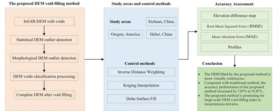
2. Materials and Methods

This section presents the detailed principles of the proposed void-filling method based on incorporating elevation outlier detection. Figure 1 illustrates the overall flow chart of the method. This method consists of the following steps: Firstly, preprocess the input DEMs to ensure that the resolution is uniform and mutually registered. This includes standardizing horizontal and vertical datum, resampling the external DEM to match the raw DEM resolution, and achieving precise registration through the iterative closest point (ICP) principle. This preprocessing ensures consistency between the area represented by the external DEM data obtained during void filling and the desired area. Secondly, DEM outlier detection and removal, explained in detail below, is applied to eliminate incorrect elevation values in raw DEM. Thirdly, DEM void filling should retain and utilize the raw DEM data as much as possible, and only introduce external DEM when the lack of external data assistance will lead to poor results. We found that smaller voids can be recovered well by interpolation, but the filling effect is poor when the voids are larger. According to the need to introduce external data to fill DEM voids, they are divided into two categories: large voids and small voids. When the void is small, simple interpolation is enough, so there is no need to introduce external data [34]. Theoretically, the size of the voids that interpolation can handle is different under different terrain conditions. The flatter the terrain, the wider the range in which interpolation can work [14]. For the convenience of calculation, this paper uses a threshold to classify large voids and small voids, which has proven to be a feasible approach in DEM void filling tasks [34]. Experiments suggest that this threshold is 16 pixels in mountainous areas; we used this fixed threshold in subsequent experiments. A void connected domain with more than 16 pixels is considered a large void, and vice versa, a small void. Finally, the DSF method is employed to fill the large voids, while IDW interpolation is used to fill the small voids. Combine the filling results of large and small voids to obtain the complete DEM finally filled by this method. IDW is an algorithm with a simple principle and will not be introduced here. Therefore, the two most important parts of the method, DEM outlier detection and removal and DSF, will be introduced in detail below.

2.1. DEM Outlier Detection and Removal

Comprehending the concept and origins of elevation outliers enhances the precision of finding solutions. Elevation outliers, or aberrant elevation values within a DEM, significantly deviate from actual elevations. Manifesting as jumps, bulges, depressions, or erratic trends, they commonly arise in undulating local terrains with low image coherence, resulting in unwrapping failures [35,36]. Typically, they manifest in the vicinity of extensive voids, as illustrated in Figure 2. The chaotic colors in (a) and dark hues in (b) indicate the presence of numerous elevation outliers surrounding voids in the area.
The detection and removal of DEM elevation outliers include two parts based on statistical principles and morphological principles, respectively. After outlier detection based on statistical and morphological principles, the elevation outliers in the raw InSAR-DEM were well detected. They will be treated as data voids and subsequently merged with the raw data voids. The following are two consecutive steps for DEM elevation outlier detection and removal: The processed DEM will be input into the next step.

2.1.1. DEM Outlier Removal Based on Statistical Detection

Notably, existing methods for detecting DEM elevation outliers share a common trait—utilizing the statistical characteristics of elevation points as the detection foundation [28,31,37]. Motivated by this, we propose a statistical method for detecting elevation errors suitable for InSAR-DEM. In optical DEMs, reversing the reference and target images generates two DEMs for comparison. Similarly, InSAR-produced DEMs can be compared with existing external DEMs, assuming consistent conditions. Deviations between the two DEMs are expected due to them describing the same terrain with theoretically limited fluctuations. In theory, if neither the InSAR-DEM nor the external DEM contain systematic errors, the elevation difference between the two should be normally distributed. Then the point where the elevation difference is far away from the mean difference between InSAR-DEM and external DEM can be considered to have a very small probability of occurrence, so it is considered an outlier. Three times the standard deviation is a commonly used criterion in statistics for detecting outliers [38], so we used this standard as the basis for statistical detection principles. It must be noted that the multiple of the standard deviation does not necessarily have to be 3. The larger the multiple, the smaller the number of outliers detected. The smaller the multiple, the greater the possibility of removing reliable points. The experimental recommendation is to set it between 2 and 4. In addition, the normalized median absolute deviation (NMAD) can also be tried as a threshold, which will not be listed here [39]. Formulae (1)–(4) derive the statistical outlier detection principle of three times the standard deviation, with d e m r a w being raw DEMs, d e m e x t e r n a l being the external DEM, d being the difference between the two DEMs, σ being the standard deviation of the difference, and μ being the mean difference. Figure 3 further illustrates the statistical removal principle graphically.
d = d e m r a w d e m e x t e r n a l
σ = d 2 n
μ = d n
d i μ > 3 σ , i o u t l i e r s d i μ 3 σ , i o u t l i e r s

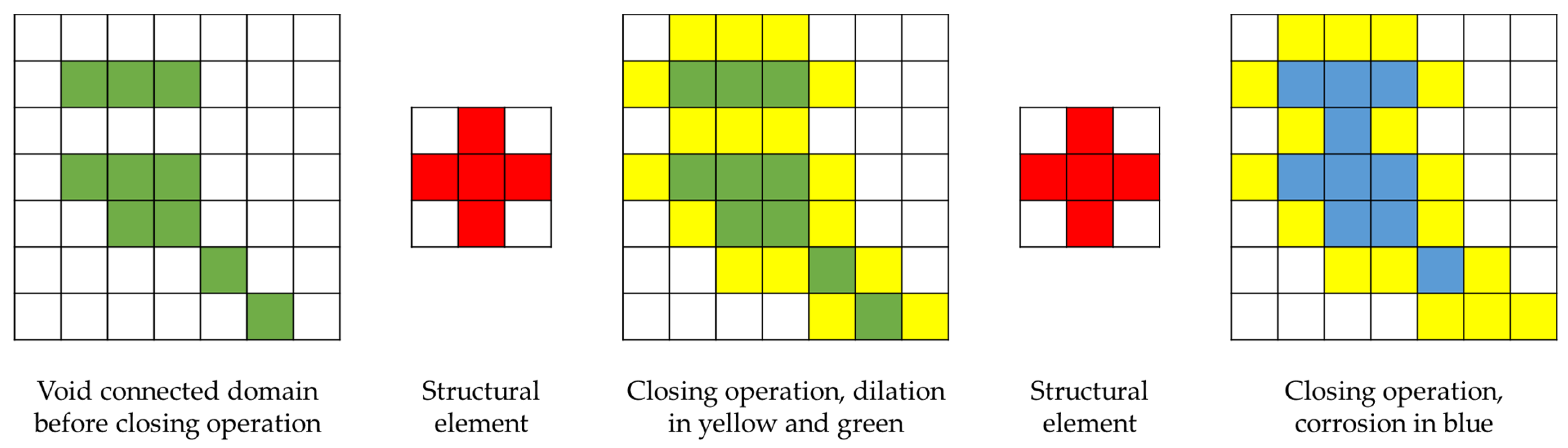
2.1.2. DEM Outlier Removal Based on Morphological Detection

Ideally, statistical principles would be sufficient to detect elevation outliers, but the actual situation is much more complex. Due to the disparate acquisition periods of external DEMs and raw DEMs, coupled with the generally limited accuracy of external DEMs, a substantial number of elevation outliers persist around voids even after statistical detection. As void filling heavily relies on the elevation values in proximity to voids, more meticulous detection of these outliers is imperative. To address this, elevation outlier detection based on morphological principles is proposed. Landform segmentation can be performed using morphological operations on DEM, which proves the potential of morphological principles to assist in DEM processing [40].
Morphological detection of elevation outliers consists of the following steps: Firstly, convert the DEM with voids after detecting elevation outliers based on the above statistical principles into a binary image. Where there is data, it is assigned a value of 0, and where there is no data, it is assigned a value of 1. Secondly, dilation and corrosion operations are performed on this binary image, which are collectively called the closing operation. The dilation operation can fill in some graphics defects, and the erosion operation can remove protruding burrs on some graphics [41]. The combination of dilation and corrosion allows adjacent small voids to be merged and void boundaries to be smoother. Specific examples of dilation and corrosion operations are shown in Figure 4. Thirdly, the changed points after morphological processing are compared with the coherence during the InSAR-DEM production process. If the standards are met, the morphological processing results will be retained. If the standards are not met, the morphological processing results will be cancelled. The changing points include the increase and decrease in void points. Only the increased points that are less than the coherence threshold meet the standard, and the decreased points that are greater than the coherence threshold meet the standard. Because morphological processing lacks a theoretical foundation related to DEM, adding coherence constraints can prevent arbitrary processing. The selection of the coherence threshold is empirical. In this article, it is selected as 0.8 through experiments, which is also applicable in most cases. Finally, we can obtain a binary image after morphological operations and coherence constraints, in which the range of voids is updated. The newly added non-zero value points in this binary map are the morphological detection results of elevation outliers.

2.2. Delta Surface Fill

Conventional void filling addresses only the data inconsistency at a void’s edge, potentially yielding inaccuracies. The DSF method aims to globally adjust all external data filled into a void, extending beyond a void’s edge adjustment [13]. This involves computing the difference between raw data and external auxiliary data within a specified overlap range along the void’s edge. As mentioned before, the DSF method is used to fill large voids. Here we take the example of filling a large void. The method encompasses the following steps:
  • Computing the delta surface of raw DEMs and external DEMs;
  • Internal filling of delta surface voids;
  • Delta surface voids’ edge interpolation;
  • Combining external DEMs and the delta surface.
Firstly, a difference is made between the raw DEM and the external DEM. Secondly, large voids in the delta surface are identified, and a fixed value is assigned to their centers. The fixed value assigned to void centers is the average of the delta surface within a certain outward range. The range size relates to the local terrain complexity and DEM resolution, with an experimental recommendation of 5–15 pixels. Thirdly, interpolate the remaining voids in the delta surface using the IDW method for a smooth transition. Lastly, add and merge the delta surface with the external DEM to obtain the DSF filling result. Figure 5 elucidates the DSF implementation process.

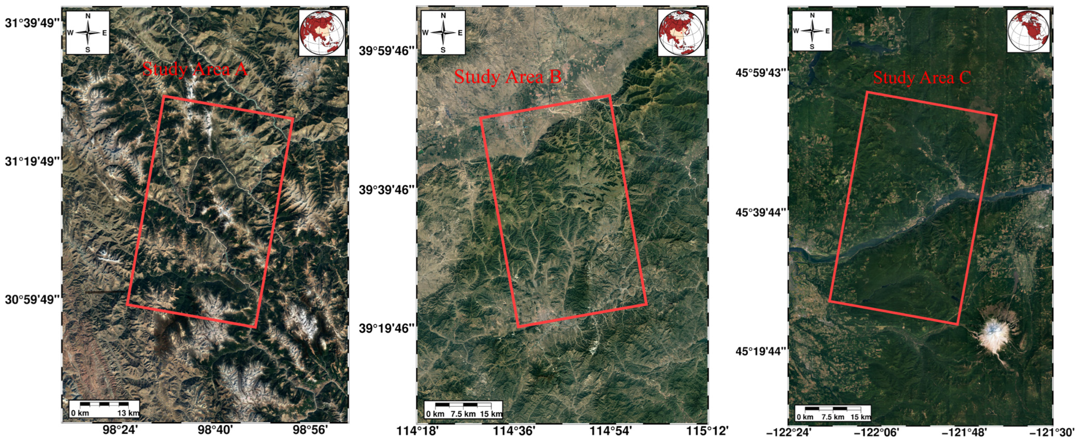
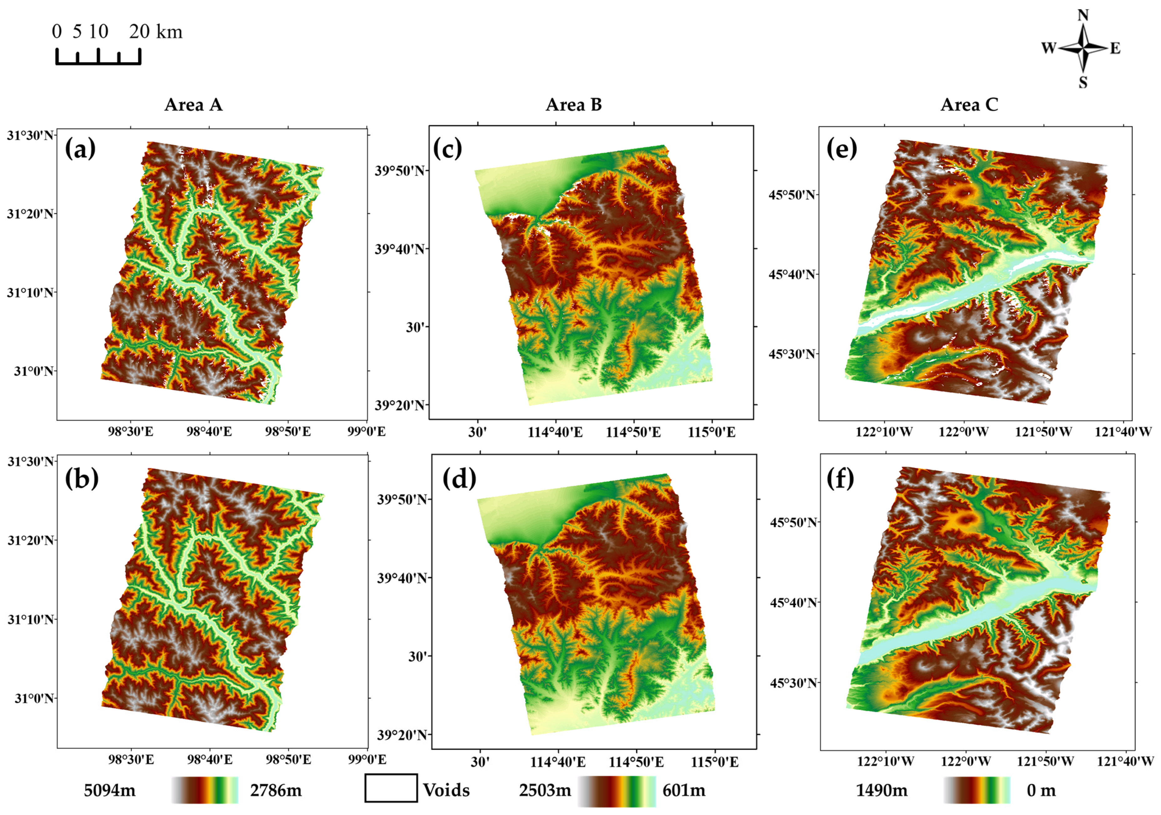
2.3. Study Area and Experimental Data

Since the outstanding innovation of this method is the inclusion of elevation outlier detection, mountainous areas with many elevation outliers are the terrain scenarios mainly effective for. In plain areas, the effect of this method is close to that of the traditional DSF method. In addition, if the void filling process is used to process the voids in the water area DEM, the elevation obtained will not be a horizontal plane. The processing of the water area DEM is generally completed by water Flattening [34]. Taking comprehensive considerations into account, we used three different mountainous terrains to test the performance of this method. In order to assess the practical efficacy of the proposed method, a real-data experiment was undertaken, centered on the challenges associated with DEM production in mountainous regions known for prevalent data voids. Three TanDEM-X satellite datasets were chosen for this investigation. The reference DEMs come from the ALOS PALSAR DEM with a 12.5 m resolution and the USGS 3DEP LiDAR DEM with a 10 m resolution [42], which are the highest quality DEMs that can be collected in their respective areas. The evaluation shows that both ALOS PALSAR DEM and LiDAR DEM have high accuracy and are sufficient to estimate the void filling effect in InSAR-DEM [43,44]. Figure 6 displays the geographical location of the study area via an optical image, delineated by a red rectangular box. Figure 7 presents raw TanDEM-X satellite-derived DEMs (Figure 7a,c,e) generated through interferometry processing, alongside high-precision ground verification DEM data (Figure 7b,d,f). Table 1 gives detailed information about prepared datasets. Leveraging ground verification data enables stereotypical analysis and comparison, as well as facilitating a comprehensive, quantitative, and detailed assessment of different methods for addressing the void-filling task.

3. Results

3.1. Void-Filling Results via Different Methods

There are both traditional methods and deep learning methods for void filling in DEM. Deep learning methods have many application cases in the field of DEM void filling, such as void filling using GAN networks. Deep learning methods can sometimes achieve better performance than traditional methods, but this performance is highly related to the training data and network parameters and is not as stable and reliable as traditional methods [26]. The method we proposed focuses on performance in large-scale DEM void-filling tasks, and deep learning methods do not yet meet this requirement. Therefore, only representative traditional methods are selected for comparative analysis. In the traditional DEM void-filling methods, two principal approaches to void filling exist: The first entails employing interpolation methods to address voids devoid of external auxiliary data. Representative methods within this category include the IDW and kriging interpolation techniques. The second approach involves resolving inconsistencies between the DEM and external auxiliary data by employing external auxiliary data to fill the voids. Various types of external auxiliary data are available for this path, with DEMs being the most commonly utilized. A well-established and acknowledged method for this purpose is the DSF method. Consequently, in our experiment, we opted for the IDW, kriging, and DSF methods as traditional group comparison methods. The external DEM, sourced from Copernicus, possesses a 30 m resolution. Data preprocessing involves resampling external source DEMs and aligning different source DEMs, ensuring a uniform resolution and reference datum for external sources and raw DEMs, and facilitating meaningful comparisons.
To observe methodological nuances, two small, rugged mountainous areas were chosen in all of areas A, B and C for meticulous analysis and comparison. Figure 8 depicts the locations of these six areas, illustrating the voids’ spatial extent before and after elevation outlier detection by method in this article. The white background in Figure 8 indicates DEM voids. The first row displays raw DEM void areas, while the second row exhibits void areas after elevation outlier removal. After detection, void areas expand, connecting some initially fragmented void groups and rendering void shapes more regular. Generally, elevation values surrounding voids bear low reliability, and elevation outlier detection yields additional results around voids, aligning with the original purpose of elevation detection. Accurate elevation outlier detection forms the basis for reliable subsequent filling. Consistent detection outcomes and theoretical expectations underpin subsequent experimental procedures.
Table 2 further details the proportions of pixels with distinct elevation values in a DEM, categorized as raw DEM void pixels, detected outlier pixels, and reliable area pixels. The proportions of detected elevation outliers exhibit significant variations across the six areas, influenced by distinct raw void proportions and elevation outlier conditions. The objective of assessing these proportions is to discern changes in filling accuracy and the affected elevation value area. Notably, the proportion of detected elevation outliers does not signify the accuracy of detection or filling. And the proposed method relies on the void mask after elevation outlier detection, while the three traditional methods use the raw void mask in the following experiments.
Subsequently, the filling of voids in the six areas was executed using three traditional methods and the proposed approach, with the results depicted in Figure 9. Examination of the raw DEMs reveals concentrated voids in regions of abrupt terrain changes, presenting a substantial challenge for void filling due to their considerable size. In such scenarios, mere interpolation proves ineffective. Both the IDW and kriging methods yield similar interpolation outcomes, generating textures within the voids that deviate from the terrain. The DSF method, aided by an external DEM, mitigates the formation of such inconsistent textures. Nonetheless, noticeable elevation disorders and errors surround the raw voids in the DSF results. The proposed method rectifies these discrepancies within DSF, yielding visually continuous and smooth filling results. Moreover, in comparison with the reference DEM, the proposed method demonstrates complete consistency in terrain texture. Despite the higher original resolution of reference DEMs, the proposed method retains more terrain details.

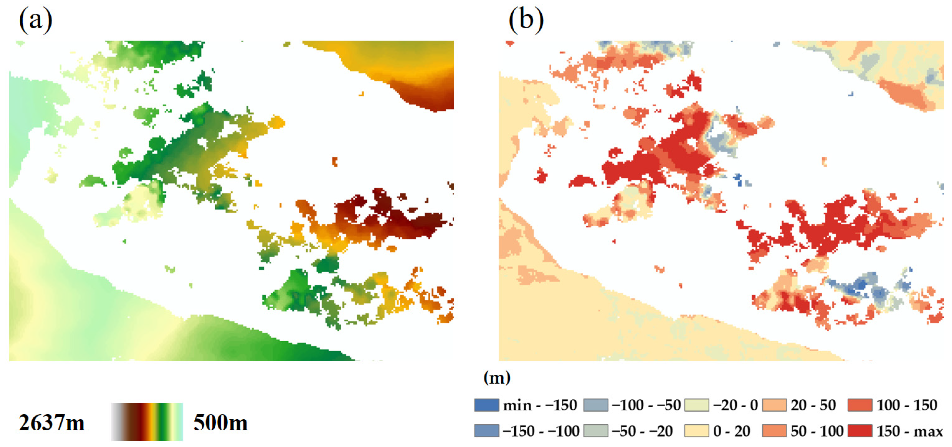
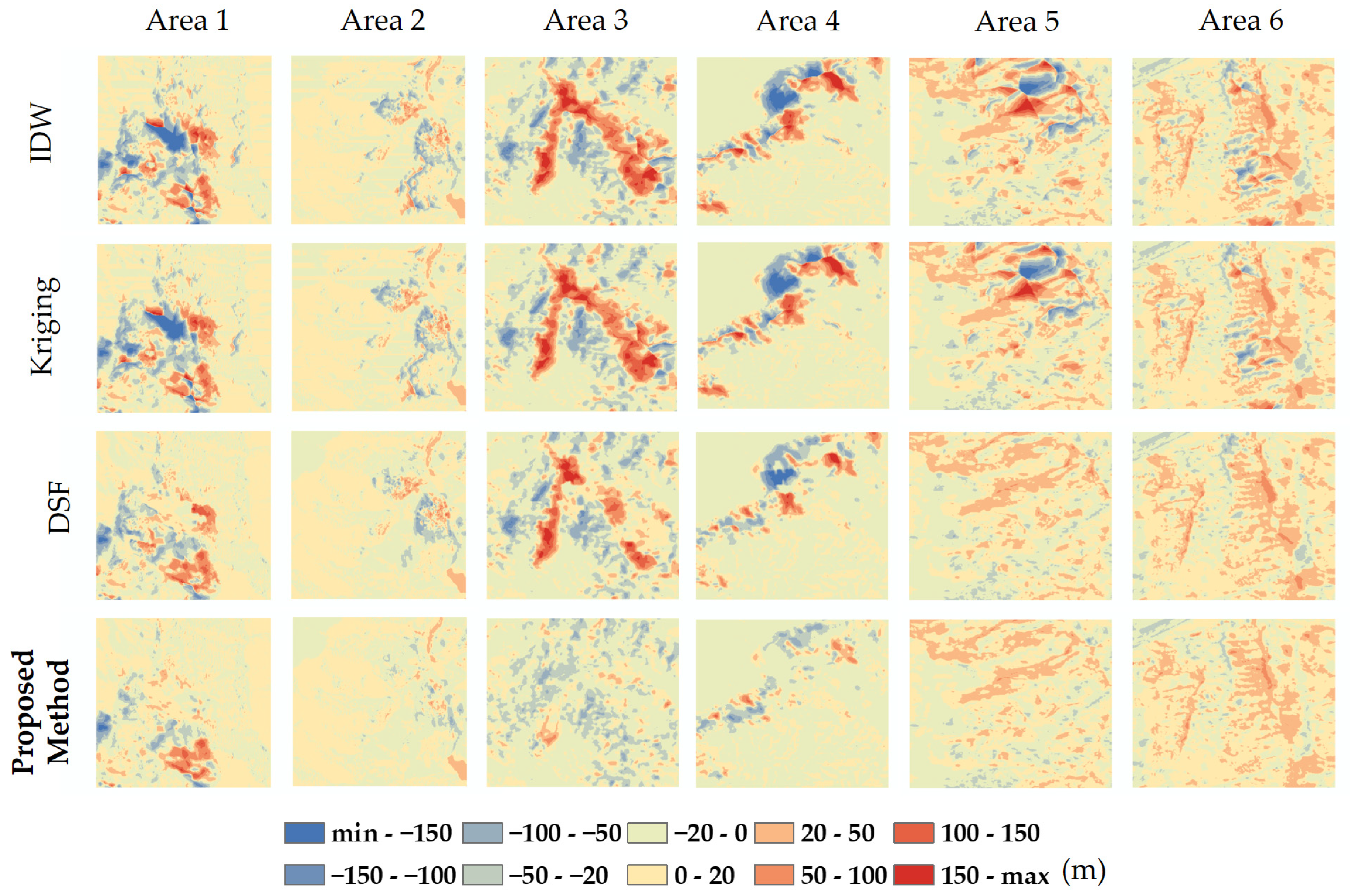
3.2. Elevation Difference Analysis

DEM data exhibits a broad value range, spanning from hundreds to thousands of meters, with the void-filling-induced floating data range typically confined within tens of meters. Consequently, the disparities in DEM-filled elevation values are inadequately discerned in an elevation map mirroring the vast DEM range. A mere DEM comparison proves insufficient for a comprehensive method evaluation. Preferably, a more effective approach involves distinguishing void-filling outcomes from the reference DEM to derive an elevation difference map.
Figure 10 contrasts the filling results of different methods with reference DEMs, presenting respective elevation difference maps. Color classification is based on the difference in magnitude, with darker colors indicating greater discrepancies. Across all areas, the difference maps exhibit a characteristic wherein the absolute value of most elevation differences hovers around 0, signifying successful co-registration. The IDW and kriging methods manifest the darkest colors, particularly around raw DEM voids, revealing a pivotal limitation in the absence of external data. Without precise void area information, void elevation data cannot be accurately reconstructed. Introducing external data through the DSF method significantly reduces the absolute value of elevation differences within voids, underscoring the imperative nature of external auxiliary data. Lastly, the proposed method further diminishes absolute elevation differences by eliminating elevation outliers, almost entirely rectifying a substantial number of errors. In comparison to all three traditional methods, the proposed method closely aligns with reference DEMs in void reconstruction, demonstrating superior elevation difference performance.
In addition to visually presenting elevation differences, the difference map facilitates the quantitative analysis of void-filling accuracy through commonly used indicators—the root mean squared error (RMSE) and mean absolute error (MAE) [14,45]. They are calculated as follows:
R M S E = 1 n i = 1 n h i H i 2
M A E = 1 n i = 1 n h i H i
h i and H i represent the filled DEM elevation and reference DEM elevation of the i-th point, and n represents the total number of elevation points. This research incorporates these indicators, providing Table 3 and Table 4. The IDW and kriging methods exhibit the highest RMSE values, whereas the DSF method shows a decline, and the proposed method consistently demonstrates the smallest RMSE in each region, aligning with previous analyses. We selected the best-performing DSF method from the comparison methods for further comparison and calculated the RMSE improvement ratio of the proposed method relative to the DSF method. In the six different enlarged areas selected, the degree of improvement ranges from 7.87% to 51.87%. This improvement correlates with the local area’s elevation outliers. The MAE results in Table 4 align with the RMSE analysis in Table 3 and will not be reiterated.

3.3. Important Terrain Void-Filling Performance Analysis by Profile

DEMs serve a crucial role in extracting and depicting significant terrain changes and features, where the discontinuity and reasonableness of terrain transformations are pivotal considerations. Drawing profiles of DEMs along selected cross-section lines at key locations provides a viable means with which to assess these factors. In Figure 11, two orthogonal sections were extracted from each of the aforementioned six small areas, and corresponding elevation change curves were plotted below. Cross-section line selection criteria involve opting for lines passing through void centers with heightened complexity and choosing two orthogonal lines to ensure sample representativeness, offering multidimensional insights. Figure 11 illustrates cross-section drawing using different methods: three colored dotted lines correspond to the traditional methods, the green solid line represents the proposed method, and the red solid line represents the reference DEM.
The proposed method’s profile exhibits the highest consistency with the reference DEM. While local elevation changes lack the detailed precision of the reference DEM, they generally capture accurate terrain characteristics. Several phenomena associated with the proposed method warrant in-depth exploration. Firstly, in raw DEMs with no void areas (depicted as a white background), the three traditional methods maintain complete consistency since they preserve raw data values. The proposed method diverges from these three traditional methods due to elevation outlier removal, resulting in changes that align the outcome more closely with the reference DEM. Secondly, within raw data void areas (gray background value), DSF and the proposed methods produce similar results, converging toward greater similarity within large voids and ultimately achieving consistency. This similarity arises from both methods using the same external DEM for filling. The difference is mainly reflected in the transition of the edges of the voids; the proposed method’s transition is more natural and aligns with reality. Thirdly, the filling outcomes of the IDW and Kriging methods are nearly identical, with minor distinctions. This uniformity arises from the shared configuration in the experiment’s interpolation process, utilizing common parameters such as interpolation reference point selection, the search point method, and interpolation order. While acknowledging that different interpolation parameters yield diverse outcomes, this research strives for comparability by employing shared parameters among methods. The quantitative results in Table 5 also indicate that the proposed method achieves lower elevation differences than the other methods.
In the void-filling task within the experimental area, the analysis of filling results, elevation differences, and profiles indicates that the proposed method surpasses traditional methods qualitatively and quantitatively.

4. Discussion

4.1. The Impact of Elevation Outlier Removal on DEM Void Filling

Whether it involves interpolation or external auxiliary data, the quality of raw DEM data significantly influences void-filling results. Interpolation-based void filling relies on raw DEMs for interpolating voids. Void filling with external data assistance is also contingent on the raw DEM’s quality for two reasons: First, the filling result borrows the trend surface of external auxiliary data, necessitating a task akin to ‘registering’ external data in raw DEM. Second, at void edges, a transition task resembling interpolation principles is inevitable.
Prior to void filling, ensuring the reliability of raw DEMs is crucial. In some regions, InSAR-produced DEMs exhibit elevation outliers, as depicted in Figure 2, resistant to resolution through coherence masks during interferometry processing. Addressing this concern, a void-filling method incorporating elevation outlier detection was introduced. Figure 8 illustrates void mask changes pre- and post-elevation outlier detection, highlighting the imperative nature of outlier detection. After detection, the remaining DEM elevation values are comparatively reliable, enhancing DEM quality and refining void areas for an easier void-filling process. Elevation outlier removal notably improves void-filling efficacy, as supported by Table 3 and Table 4, and Figure 10. Extending the elevation outlier detection concept to other void-filling methods, performed prior to filling, holds potential for progress. While this study concentrates on evaluating the proposed void-filling method’s impact, further exploration of combining elevation outlier detection with traditional void-filling methods is a prospective research direction.

4.2. Suitable Situations and Future Improvement Directions of the Proposed Method

This method is very effective in quickly filling DEM voids in large-scale mountainous DEMs, with two key characteristics. Firstly, it is tailored for the adaptability of DEM terrain, particularly well-suited for rugged mountainous areas prone to data voids, often of considerable size. Traditional interpolation methods falter in addressing extensive voids, whereas the proposed method adeptly handles both large and small voids. In order to explore whether it is necessary to divide the voids into large voids and small voids for separate processing, we conducted an experiment in area C. And the accuracy of the statistical results for the two processing strategies are listed in Table 6. It must be noted that the difference between the two strategies is only in the small voids, so the statistical accuracy here is the accuracy within the small voids rather than the entire DEM. Experiments show that, compared to processing all voids uniformly, dividing the voids into large and small voids and processing them separately can improve the accuracy of the results. The difficulty and effect of the DSF void-filling method used in this study for a large void depend on whether the elevation around the void is reliable. Therefore, although the void becomes larger after the elevation outliers are removed, the elevation around the void becomes more reliable, the difficulty of filling is reduced, and the effect is improved.
Secondly, the method is tailored for DEM data with locally poor quality, such as low coherence or difficulty in phase unwrapping due to mountainous terrain and vegetation. The elevation outlier removal step effectively eliminates poor-quality elevation points, mitigating adverse effects. In other terrain scenarios, the advantages of this method are not obvious. For example, in plain areas, the DEM obtained by InSAR has high quality and reliability and few elevation outliers. The effect of this method is close to that of the DSF method. For another example, in the water areas, the filled water terrain is messy, which is inconsistent with the actual situation of the water being flat and requires special water flattening processing.
Regarding the selection and impact of external source DEM, It’s essential to clarify that, although in most cases, the resolution and accuracy of external DEMs are lower than those of raw DEMs, using a small amount in voids is a viable alternative. In void-filling tasks for large voids, the quality of the selected external DEM significantly impacts the reconstructed elevation quality within the void. Opting for a high-quality DEM is imperative to ensure void-filling quality. Additionally, the external DEM resolution should not significantly differ from that of raw DEMs to prevent the occurrence of a ‘patch’ effect caused by resolution disparities in void reconstruction.
Every method has limitations, and the proposed method is no exception. These limitations also point to areas for future improvement and can be outlined in two key aspects: on the one hand, by employing methods like terrain factor extraction and raw DEM-based analysis to enhance the accuracy of elevation outlier detection; on the other hand, by enhancing the resolution of the external DEM by integrating optical images or SAR intensity maps, replacing the basic resampling step to ensure improved data quality consistency in the filling results.

5. Conclusions

In this research, the concept of DEM elevation outlier detection and removal was introduced into the traditional DEM void-filling process, and a void-filling method based on incorporating elevation outlier detection is proposed. The proposed method detected and removed outliers existing in raw DEMs by combining statistical principles and morphological principles, thereby improving the quality of void filling. Three experimental datasets from Sichuan, China; Hebei, China; and Oregon, America, were applied to conduct real experiments. The three classic traditional methods of IDW, kriging, and DSF were selected as control methods. The experimental results show that, compared with traditional methods, both qualitative and quantitative filling results have been greatly improved. Compared with the DSF method, the RMSE of the filling results by the proposed method has improved by 7.87% to 51.87%. The proposed method can solve the problems of elevation outliers existing in raw DEMs and achieve significant improvements in filling quality. In addition, the analysis also found that, this method has its preferred application situation, which is rugged mountainous areas. And the elevation outlier detection and removal method in this article could be generalized and applied to other DEM void-filling methods to improve the quality of DEM void filling in different situations.

Author Contributions

Conceptualization, Z.H., R.G. and J.H.; methodology, Z.H. and J.H.; software, R.G. and J.H.; validation, Z.H., R.G. and J.H.; formal analysis, Z.H. and R.G.; investigation, Y.Y., K.J. and L.L.; resources, R.G., J.H. and H.F.; data curation, Z.H., R.G. and H.F.; writing—original draft preparation, Z.H., R.G. and J.H.; writing—review and editing, all authors; visualization, Z.H., Y.Y. and K.J.; supervision, R.G., J.H. and H.F.; project administration, R.G. and J.H.; funding acquisition, R.G. and J.H. All authors have read and agreed to the published version of the manuscript.

Funding

This work was supported by the National Natural Science Foundation of China under grants 42030112 and 42201432, the science and technology innovation program of Hunan Province (No. 2022RC3042), and the science and technology innovation program of Fujian Province (No. 2021Y3001).

Data Availability Statement

The original contributions presented in the study are included in the article, further inquiries can be directed to the corresponding author.

Acknowledgments

The Authors would like to thank DLR for providing the TanDEM-X data and USGS for providing LiDAR DEM (U.S. Geological Survey, 2023, 1/3rd arc-second Digital Elevation Models (DEMs)—USGS National Map 3DEP Downloadable Data Collection: U.S. Geological Survey).

Conflicts of Interest

The authors declare no conflicts of interest.

References

  1. Lakshmi, S.E.; Yarrakula, K. Review and critical analysis on digital elevation models. G Eofizika 2018, 35, 103–284. [Google Scholar] [CrossRef]
  2. Tarolli, P. High-resolution topography for understanding Earth surface processes: Opportunities and challenges. Geomorphology 2014, 216, 295–312. [Google Scholar] [CrossRef]
  3. Badura, J.; Przybylski, B.A. Application of digital elevation models to geological and geomorphological studies-some examples. Przegląd Geol. 2005, 53, 977–983. [Google Scholar]
  4. Wechsler, S. Uncertainties associated with digital elevation models for hydrologic applications: A review. Hydrol. Earth Syst. Sci. 2007, 11, 1481–1500. [Google Scholar] [CrossRef]
  5. Racoviteanu, A.E.; Manley, W.F.; Arnaud, Y.; Williams, M.W. Evaluating digital elevation models for glaciologic applications: An example from Nevado Coropuna, Peruvian Andes. Glob. Planet. Chang. 2007, 59, 110–125. [Google Scholar] [CrossRef]
  6. Zhou, G.; Bao, X.; Ye, S.; Wang, H.; Yan, H. Selection of optimal building facade texture images from UAV-based multiple oblique image flows. IEEE Trans. Geosci. Remote Sens. 2020, 59, 1534–1552. [Google Scholar] [CrossRef]
  7. Geymen, A. Digital elevation model (DEM) generation using the SAR interferometry technique. Arab. J. Geosci. 2014, 7, 827–837. [Google Scholar] [CrossRef]
  8. Zheng, W.; Hu, J.; Lu, Z.; Hu, X.; Sun, Q.; Liu, J.; Zhu, J.; Li, Z. Enhanced Kinematic Inversion of 3-D Displacements, Geometry, and Hydraulic Properties of a North-South Slow-Moving Landslide in Three Gorges Reservoir. J. Geophys. Res. Solid Earth 2023, 128, e2022JB026232. [Google Scholar] [CrossRef]
  9. Hirt, C. Artefact detection in global digital elevation models (DEMs): The Maximum Slope Approach and its application for complete screening of the SRTM v4.1 and MERIT DEMs. Remote Sens. Environ. 2018, 207, 27–41. [Google Scholar] [CrossRef]
  10. Dowding, S.; Kuuskivi, T.; Li, X. Void fill of SRTM elevation data—Principles, processes and performance. In ASPRS Images to Decision: Remote Sensing Foundation for GIS Applications; ASPRS: Bethesda, MD, USA, 2004; pp. 12–16. [Google Scholar]
  11. Ma, H.; Zhou, W.; Zhang, L. DEM refinement by low vegetation removal based on the combination of full waveform data and progressive TIN densification. ISPRS J. Photogramm. Remote Sens. 2018, 146, 260–271. [Google Scholar] [CrossRef]
  12. Yan, W.Y. Scan line void filling of airborne LiDAR point clouds for hydroflattening DEM. IEEE J. Sel. Top. Appl. Earth Obs. Remote Sens. 2021, 14, 6426–6437. [Google Scholar] [CrossRef]
  13. Grohman, G.; Kroenung, G.; Strebeck, J. Filling SRTM voids: The delta surface fill method. Photogramm. Eng. Remote Sens. 2006, 72, 213–216. [Google Scholar]
  14. Reuter, H.I.; Nelson, A.; Jarvis, A. An evaluation of void-filling interpolation methods for SRTM data. Int. J. Geogr. Inf. Sci. 2007, 21, 983–1008. [Google Scholar] [CrossRef]
  15. Luedeling, E.; Siebert, S.; Buerkert, A. Filling the voids in the SRTM elevation model—A TIN-based delta surface approach. ISPRS J. Photogramm. Remote Sens. 2007, 62, 283–294. [Google Scholar] [CrossRef]
  16. Hall, O.; Falorni, G.; Bras, R.L. Characterization and quantification of data voids in the shuttle radar topography mission data. IEEE Geosci. Remote Sens. Lett. 2005, 2, 177–181. [Google Scholar] [CrossRef]
  17. Dong, G.; Huang, W.; Smith, W.A.; Ren, P. A shadow constrained conditional generative adversarial net for SRTM data restoration. Remote Sens. Environ. 2020, 237, 111602. [Google Scholar] [CrossRef]
  18. Wecker, L.; Samavati, F.; Gavrilova, M. Contextual void patching for digital elevation models. Vis. Comput. 2007, 23, 881–890. [Google Scholar] [CrossRef]
  19. Ling, F.; Zhang, Q.; Wang, C. Filling voids of SRTM with Landsat sensor imagery in rugged terrain. Int. J. Remote Sens. 2007, 28, 465–471. [Google Scholar] [CrossRef]
  20. Crippen, R.E.; Hook, S.J.; Fielding, E.J. Nighttime ASTER thermal imagery as an elevation surrogate for filling SRTM DEM voids. Geophys. Res. Lett. 2007, 34. [Google Scholar] [CrossRef]
  21. Hogan, J.; Smith, W.A. Refinement of digital elevation models from shadowing cues. In Proceedings of the 2010 IEEE Computer Society Conference on Computer Vision and Pattern Recognition, San Francisco, CA, USA, 13–18 June 2010; pp. 1181–1188. [Google Scholar]
  22. Dong, G.; Huang, W.; Smith, W.A.; Ren, P. Filling voids in elevation models using a shadow-constrained convolutional neural network. IEEE Geosci. Remote Sens. Lett. 2019, 17, 592–596. [Google Scholar] [CrossRef]
  23. Jarvis, A.; Reuter, H.I.; Nelson, A.; Guevara, E. Hole-Filled SRTM for the Globe Version 4. The CGIAR-CSI SRTM 90 m Database. 2008, Volume 15, p. 5. Available online: http://srtm.csi.cgiar.org (accessed on 3 November 2023).
  24. Huber, M.; Osterkamp, N.; Marschalk, U.; Tubbesing, R.; Wendleder, A.; Wessel, B.; Roth, A. Shaping the global high-resolution TanDEM-X digital elevation model. IEEE J. Sel. Top. Appl. Earth Obs. Remote Sens. 2021, 14, 7198–7212. [Google Scholar] [CrossRef]
  25. Robinson, N.; Regetz, J.; Guralnick, R.P. EarthEnv-DEM90: A nearly-global, void-free, multi-scale smoothed, 90m digital elevation model from fused ASTER and SRTM data. ISPRS J. Photogramm. Remote Sens. 2014, 87, 57–67. [Google Scholar] [CrossRef]
  26. Li, S.; Hu, G.; Cheng, X.; Xiong, L.; Tang, G.; Strobl, J. Integrating topographic knowledge into deep learning for the void-filling of digital elevation models. Remote Sens. Environ. 2022, 269, 112818. [Google Scholar] [CrossRef]
  27. Qiu, Z.; Yue, L.; Liu, X. Void filling of digital elevation models with a terrain texture learning model based on generative adversarial networks. Remote Sens. 2019, 11, 2829. [Google Scholar] [CrossRef]
  28. López, C. Improving the elevation accuracy of digital elevation models: A comparison of some error detection procedures. Trans. GIS 2000, 4, 43–64. [Google Scholar] [CrossRef]
  29. Chen, C.; Liu, F.; Li, Y.; Yan, C.; Liu, G. A robust interpolation method for constructing digital elevation models from remote sensing data. Geomorphology 2016, 268, 275–287. [Google Scholar] [CrossRef]
  30. Chen, C.; Li, Y. A robust multiquadric method for digital elevation model construction. Math. Geosci. 2013, 45, 297–319. [Google Scholar] [CrossRef]
  31. Schultz, H.; Riseman, E.M.; Stolle, F.R.; Woo, D.-M. Error detection and DEM fusion using self-consistency. In Proceedings of the Seventh IEEE International Conference on Computer Vision, Kerkyra, Greece, 20–27 September 1999; pp. 1174–1181. [Google Scholar]
  32. Zhang, K.; Gann, D.; Ross, M. Detection of Low Elevation Outliers in TanDEM-X DEMs With Histogram and Adaptive TIN. IEEE Trans. Geosci. Remote Sens. 2021, 60, 5101213. [Google Scholar] [CrossRef]
  33. Ghannadi, M.A.; Alebooye, S.; Izadi, M.; Moradi, A. A method for Sentinel-1 DEM outlier removal using 2-D Kalman filter. Geocarto Int. 2022, 37, 2237–2251. [Google Scholar] [CrossRef]
  34. González, C.; Bachmann, M.; Bueso-Bello, J.-L.; Rizzoli, P.; Zink, M. A fully automatic algorithm for editing the tandem-x global dem. Remote Sens. 2020, 12, 3961. [Google Scholar] [CrossRef]
  35. Chukwuocha, A.C. Outlier based selection and accuracy updating of digital elevation models for urban area projects. Afr. J. Environ. Sci. Technol. 2018, 12, 258–267. [Google Scholar]
  36. Zhang, W.; Wang, W.; Chen, L. Constructing DEM based on InSAR and the relationship between InSAR DEM’s precision and terrain factors. Energy Procedia 2012, 16, 184–189. [Google Scholar] [CrossRef]
  37. Felicísimo, A.M. Parametric statistical method for error detection in digital elevation models. ISPRS J. Photogramm. Remote Sens. 1994, 49, 29–33. [Google Scholar] [CrossRef]
  38. Curran-Everett, D. Explorations in statistics: Standard deviations and standard errors. Adv. Physiol. Educ. 2008, 32, 203–208. [Google Scholar] [CrossRef] [PubMed]
  39. Höhle, J.; Höhle, M. Accuracy assessment of digital elevation models by means of robust statistical methods. ISPRS J. Photogramm. Remote Sens. 2009, 64, 398–406. [Google Scholar] [CrossRef]
  40. Sathymoorthy, D.; Palanikumar, R.; Sagar, B. Morphological segmentation of physiographic features from DEM. Int. J. Remote Sens. 2007, 28, 3379–3394. [Google Scholar] [CrossRef]
  41. Haralick, R.M.; Sternberg, S.R.; Zhuang, X. Image analysis using mathematical morphology. IEEE Trans. Pattern Anal. Mach. Intell. 1987, 532–550. [Google Scholar] [CrossRef] [PubMed]
  42. U.S. Geological Survey. 1/3rd Arc-Second Digital Elevation Models (DEMs)—USGS National Map 3DEP Downloadable Data Collection; US Geological Survey: Reston, VA, USA, 2023.
  43. Ferreira, Z.A.; Cabral, P. Vertical Accuracy Assessment of ALOS PALSAR, GMTED2010, SRTM and Topodata Digital Elevation Models. In Proceedings of the GISTAM, Online, 23–25 April 2021; pp. 116–124. [Google Scholar]
  44. Stoker, J.; Miller, B. The accuracy and consistency of 3d elevation program data: A systematic analysis. Remote Sens. 2022, 14, 940. [Google Scholar] [CrossRef]
  45. Zheng, X.; Xiong, H.; Yue, L.; Gong, J. An improved ANUDEM method combining topographic correction and DEM interpolation. Geocarto Int. 2016, 31, 492–505. [Google Scholar] [CrossRef]
Figure 1. Void-filling flow chart of the proposed method based on incorporating elevation outlier detection.
Remotesensing 16 01452 g001
Figure 2. DEM outlier example. (a) the actual elevation; (b) the residual map of (a) compared to the reference DEM.
Remotesensing 16 01452 g002
Figure 3. Statistical outlier detection scheme. (a) An example of a statistical histogram of elevation differences between an InSAR-DEM and an external DEM; elevation mean difference μ and standard deviation σ are listed; (b) A schematic diagram of outlier distribution under normal distribution, data outside the two red dashed lines represent outliers.
Remotesensing 16 01452 g003
Figure 4. Dilation and corrosion morphology operations. Examples are shown before the operation, after the dilation operation, and after the dilation and corrosion operation. Green represents the initial void range, yellow represents the void range added by the dilation operation, blue represents the void range retained after the corrosion operation, and red represents the structural elements of the morphological operation.
Remotesensing 16 01452 g004
Figure 5. DSF implementation process. Various colors: light green for DEM data, red for data voids, and pink for the delta surface. (a) is raw DEMs; (b) is external DEMs; (c) = (b) − (a) is the delta surface corresponding to step (I); (d) is the delta surface center filled in large voids by mean value, corresponding to step (II); (e) is the delta surface filled and interpolated entirely, corresponding to step (III); (f) = (b) − (e) is the filled DEM corresponding to step (IV). Red represents void pixels, pink represents elevation difference pixels, and green represents elevation pixels.
Remotesensing 16 01452 g005
Figure 6. The location of the study areas and data coverage (red rectangular box). A, B, and C are data coverage maps of the three study areas of Sichuan, Hebei, and Oregon respectively.
Remotesensing 16 01452 g006
Figure 7. Raw DEMs (a,c,e) generated by TanDEM-X and reference DEMs (b,d,f). (a,b) correspond to area A, (c,d) correspond to area B, and (e,f) correspond to area C.
Remotesensing 16 01452 g007
Figure 8. Two small areas were enlarged in area A, area B and area C, named area 1, area 2, area 3, area 4, area 5, and area 6. These areas, denoted as raw voids and voids after elevation outlier detection, will be used in subsequent experiments. The white background in the enlarged figure represents voids.
Remotesensing 16 01452 g008
Figure 9. Comparison of the filling results of six different areas using different methods. The white background in the figure represents voids.
Remotesensing 16 01452 g009
Figure 10. Enlarged view of the elevation difference of DEMs filled through different methods.
Remotesensing 16 01452 g010
Figure 11. Profile performance of enlarged figures of the six areas using different void-filling methods. The location of the section lines is indicated by purple and yellow line segments.
Remotesensing 16 01452 g011
Table 1. Detailed information about the prepared datasets.
LocationLandformDatatypeData SourceSpatial
Resolution
Image Size
(Pixels)
Void Pixels
Area ASichuan,
China
Plateau,
bare ground
Raw DEMTanDEM-X10 m5538 × 4572654,907
Reference DEMALOS PALSAR12.5 m4430 × 3658-
Area BHebei,
China
Mountain,
low vegetation
Raw DEMTanDEM-X10 m6016 × 4818176,085
Reference DEMALOS PALSAR12.5 m4813 × 3854-
Area COregon,
America
Mountain,
High vegetation
Raw DEMTanDEM-X10 m6043 × 4986807,757
Reference DEMLiDAR10 m6054 × 6001-
Table 2. Statistics on the pixel proportion of voids, detected outliers, and reliable area for different study areas.
Raw DEM Voids
(%)
Detected Outliers
(%)
Reliable Area
(%)
Area 118.728.1873.10
Area 210.745.9483.32
Area 316.8217.1666.02
Area 413.526.9579.53
Area 527.669.9762.37
Area 618.2911.2370.48
Table 3. Elevation RMSE of different void-filling methods in six areas. The data in bold in the table are the best performing methods.
RMSE (m)Improvement (%)
IDWKrigingDSFProposed MethodCompared to DSF
Area 147.4047.0026.7622.1517.23
Area 216.1815.8012.828.7331.90
Area 346.6046.3938.5818.5751.87
Area 439.1738.9029.8215.0449.56
Area 533.7533.1016.6515.347.87
Area 623.4423.0319.3517.638.89
Table 4. Elevation MAE of different void-filling methods in six areas. The data in bold in the table are the best performing methods.
MAE (m)Improvement (%)
IDWKrigingDSFProposed MethodCompared to DSF
Area 121.9821.7714.1811.1421.44
Area 29.128.967.185.6721.03
Area 328.4328.2922.8713.5840.62
Area 417.4417.3913.248.4835.95
Area 520.7020.3213.1912.138.04
Area 617.3417.1315.1614.097.06
Table 5. Elevation accuracy of the selected profiles in Figure 11. The data in bold in the table are the best performing methods.
MAE of Line 1 (m) MAE of Line 2 (m)
IDWKrigingDSFProposed MethodIDWKrigingDSFProposed
Method
Area 142.4542.4620.6414.7435.1735.176.755.82
Area 217.5717.148.106.377.457.014.804.58
Area 339.9439.7834.7013.8051.7251.7240.2518.57
Area 438.8638.6127.468.3022.2622.0016.4410.84
Area 537.4636.3013.6412.5815.1015.1013.2810.67
Area 627.6026.8117.8517.2916.2915.4712.6913.30
Table 6. The accuracy statistics table for separate processing and unified processing of large and small voids. Only counts the accuracy within small voids. The data in bold in the table are the best performing methods.
RMSE (m)MAE (m)
separate large and small voids process14.5611.55
unify large and small voids process14.7211.83
Disclaimer/Publisher’s Note: The statements, opinions and data contained in all publications are solely those of the individual author(s) and contributor(s) and not of MDPI and/or the editor(s). MDPI and/or the editor(s) disclaim responsibility for any injury to people or property resulting from any ideas, methods, instructions or products referred to in the content.

