Ocean Satellite Data Fusion for High-Resolution Surface Current Maps

Abstract

Real-time reconstruction of ocean surface currents is a challenge due to the complex, non-linear dynamics of the ocean, the small number of in situ measurements, and the spatio-temporal heterogeneity of satellite altimetry observations. To address this challenge, we introduce HIRES-CURRENTS-Net, an operational real-time convolutional neural network (CNN) model for daily ocean current reconstruction. This study focuses on the Mediterranean Sea, a region where operational models have great difficulty predicting surface currents. Notably, our model showcases higher accuracy compared to commonly used alternative methods. HIRES-CURRENTS-Net integrates high-resolution measurements from the infrared or visible spectrum—high resolution Sea Surface Temperature (SST) or chlorophyll (CHL) images—in addition to the low-resolution Sea Surface Height (SSH) maps derived from satellite altimeters. In the first stage, we apply a transfer learning method which uses a high-resolution numerical model to pre-train our CNN model on simulated SSH and SST data with synthetic clouds. The observation of System Simulation Experiments (OSSEs) offers us a sufficient training dataset with reference surface currents at very high resolution, and a model trained on this data can then be applied to real data. In the second stage, to enhance the real-time operational performance of our model over previous methods, we fine-tune the CNN model on real satellite data using a novel pseudo-labeling strategy. We validate HIRES-CURRENTS-Net on real data from drifters and demonstrate that our data-driven approach proves effective for real-time sea surface current reconstruction with potential operational applications such as ship routing.

1. Introduction

The increase in the spatial resolution in both numerical models and remote sensing observations (infrared or visible image) allows for the observation of the complex, non-linear dynamics of oceanic currents. The signatures of both large-scale mesoscale eddies or meanders and submesoscale structures such as small intense eddies or filaments are identifiable, by an experienced oceanographer, in high-resolution satellite imagery of Sea Surface Temperatures (SSTs) and the visible spectrum (e.g., chlorophyll reflectance). However, these satellite observations do not provide a direct reconstruction of the ocean surface velocity field and remain incomplete due to cloud coverage and noise. Direct in situ measurements of the ocean currents (moorings, drifters or oceanographic campaigns) are sparse and cannot be used to build real-time current maps. Today, the standard method that has led to major advances in the global and continuous monitoring of ocean surface currents [1,2] is based on the geostrophic balance assumption and involves interpolating sparse and inhomogenous measurements of Sea Surface Height (SSH). However, this method suffers from a strong spatio-temporel filtering and cannot detect fine-scale structures or small submesocale eddies [3,4]. This poses significant challenges for the real-time reconstruction of surface currents both in coastal areas and in the open ocean. Detecting ocean currents is vital to our understanding of global heat exchanges, the transport of pollutants and of biogeochemical components between the coast and the open sea. Moreover, precise and reliable knowledge of daily surface currents at high resolution allows for short-term optimal ship routing [5], a low-cost/low-risk solution that can be immediately deployed to advance shipping decarbonization.

SSH, SST, chlorophyll, and other variables are connected by physical relationships determined by ocean circulation. This relationship can be exploited by combining different types of observational satellite data in a multi-modal framework. For example, SST and chlorophyll can be obtained at a high resolution (around 1 km), while interpolated SSH data from satellite altimetry are available at a coarser resolution (around 8 km in the Mediterranean Sea and around 26 km for global products). On days with minimal cloud cover, SST and visible spectra often reveal the signatures of small-scale eddies, whereas such details might be absent in low-resolution SSH interpolations. Conversely, SSH measurements can provide valuable data even in cloudy conditions, thereby supplementing SST and chlorophyll observations.

Real-time operational daily now-casts of ocean surface currents are broadly categorized into three groups: numerical modeling, satellite altimetry geostrophic currents, and new data-driven approaches. In particular, advances in AI computer vision have lead to exponential growth in data-driven methods in oceanography [6,7,8].

Numerical ocean modeling have played an essential role in representing and forecasting ocean currents [9]. These operational ocean models consist of a numerical solution to a set of partial differential equations describing the ocean dynamics, its physical properties, and the main external forces. The increase in computational power now allows for global ocean circulation models to routinely resolve oceanic currents with an horizontal resolution of around 10 km. For instance, the Mercator–Ocean model [10] assimilates data from satellite and in situ observations in real time to produce operational now-casts and forecasts of global ocean currents among other variables at 1/12° [11]. However, the reliability and accuracy of these operational models is limited by the quantity and heterogeneity of the data available for numerical assimilation, and by the assimilation scheme itself. Moreover, the spatial resolution of these operational models does not model sub-mesoscale velocity gradients. Numerical models with very high spatial resolution (about 1 km or even less) exist for regional configurations such as the Mediterranean Sea [12], the North Atlantic [13], or in the Indian Ocean [14], but the lack of ocean observations at this resolution limits the accuracy of their forecasts in operational scenarios. However, these models are very useful for studying, or analyzing a posteriori, the sub-mesoscale dynamics of the ocean, especially in coastal regions. Moreover, the accuracy and quantity of these simulated data are also great assets for neural methods trained through supervised learning.

Satellite altimetry missions such as TOPEX/POSEIDON and Jason have been a fundamental tool for measuring SSH, allowing estimation of geostrophic ocean currents [15,16,17]. As along-track altimetry measurements are sparse, methods such as the Kalman filter provide an optimal way to interpolate between observed data points [18,19]. The state-of-the-art interpolated SSH product AVISO/DUACS [20] optimally interpolates data from multiple altimetry satellites and additionally applies geophysical corrections. Geostrophic currents can then be estimated from this interpolated SSH product. Recent missions such as SWOT will improve the quality of altimetry data in the very near future [21,22] by providing wide-swath observations. Nevertheless, the daily geographic coverage of SWOT will remain sparse in the near future.

Convolutional Neural Networks (CNNs) have emerged as a groundbreaking class of deep learning models that have revolutionized the field of computer vision and image analysis. Inspired by the human visual system, CNNs are specifically designed to process and interpret visual data efficiently. These models apply convolutional operations which involve sliding a set of learnable filters over the input image to extract relevant features. These filters detect various patterns such as edges, textures, and shapes, hierarchically combining them to recognize more complex structures. Through multiple layers of convolutions interspersed with activation functions like ReLU and pooling layers, CNNs progressively learn abstract representations of the input data [23,24]. This hierarchical feature learning enables CNNs to achieve state-of-the-art performance in tasks such as image classification, object detection, and image segmentation [25].

Super Resolution (SR) has been a rapidly advancing field of application of CNNs [26], where a Low-Resolution (LR) image is upsampled into a High-Resolution (HR) version. The problem of reconstructing ocean currents from sparse SSH information and other observations is similar to other problems of super-resolution in the computer vision literature. The authors of [26] train a convolutional neural network to output a high-resolution image from a low-resolution image. In particular, skip connections are demonstrated to be useful in increasing the computational efficiency and learning local and global information for super-resolution tasks in [27].

The U-Net model introduced in [28], initially designed for biomedical image segmentation, finds wide application across many different tasks due to its convolutional architecture, skip connections, and generative capabilities. Notably, the U-Net architecture has proven useful in many tasks in oceanography, including eddy detection [29,30,31], identification of algae blooms [32,33], and detecting or classifying sea ice [34,35]. The U-Net model is also a backbone of many recent diffusion models, such as in [36], where it is used for image super-resolution.

Recent state-of-the-art methods for ocean currents reconstruction use neural networks to learn non-linear representations from satellite observations. These methods are generally trained on simulated data, and are then evaluated either on simulated data from an excluded test set or on real data such as drifters. System Simulation Experiments (OSSEs) such as [37,38,39] are based on geophysical models and have proven essential in training data-driven methods. An OSSE is a modeling experiment used to evaluate the value of a new observing system when actual observational data are not available. The OSSE setup comprises a nature run, a data assimilation system, and software tasked with simulating ‘observations’ derived from the nature run while incorporating realistic observation errors. Numerous studies train models to reconstruct SSH using simulated data from the Gulf Stream [37], such as 4DVarNet (Fablet et al. [8]) and the CNN-based method RESAC (Thiria et al. [40]). Nardelli et al. [7] use simulated data from the Mediterranean Sea [38] to reconstruct SSH and surface currents. In more recent developments, Archambault et al. [41] and Martin et al. [42,43] present training strategies for learning the SSH field without simulated data by computing loss only along the tracks of SSH observations. Self-supervised or unsupervised methods can help close the domain gap between simulations (often in precise geographical contexts) and real data at a global scale.

Estimation of currents from SST signatures has existed in the literature since the 1980s, including [44,45,46,47]. In the aforementioned studies [7,8,40,41], incorporating high-resolution SST images notably enhances SSH reconstruction. However, the SST data are affected by clouds and so the models may not achieve strong performance when the SST product is inaccurate due to high levels of clouds. Chlorophyll concentrations are also a proxy indicator of ocean currents [48,49,50]. Culoto et al. [51] use chlorophyll, SST, and SSH observation data in combination with a clustering strategy to reconstruct 3D salinity profiles. In [38], the authors provide simulated observations of chlorophyll, but to the best of our knowledge, there are no data-driven methods trained to predict ocean currents from signatures in chlorophyll distribution.

In this study, we develop a real-time operational pipeline for high-resolution ocean surface current reconstruction which outperforms standard methods (Figure 1). We train an encoder–decoder convolutional neural network with multi-modal inputs to predict the velocity field. Our model is trained using an Observing System Simulation Experiment (OSSE). In contrast to previous methods, our method can be applied to a cloudy SST images (L3 SST) rather than interpolated cloud-free SST products (L4 SST). Notably, our model showcases consistent performance when presented with either L3 (cloudy) or L4 (interpolated) SST data, a significant improvement over previous approaches. Additionally, our novel pseudo-labeling strategy allows us to fine-tune our model on real data, closing the domain gap and increasing robustness in operational applications. Moreover, our pseudo-labeling strategy allows for us to integrate alternative inputs which may not be available in OSSEs, such as chlorophyll.

To validate our results on real satellite observations, we use sparse in situ measurements obtained from drifters. Our results demonstrate that our approach leads to improved reconstruction accuracy for both current intensity and direction compared to standard methods. Furthermore, our model demonstrates promising potential for operational deployment in practical applications, particularly in optimizing ship routing.

2. Data and Methods

We train and evaluate our model using both simulated and real data from the Mediterranean Sea. In the following sections, we describe the real data used for operational applications as well as for fine-tuning our model (Section 2.1), the simulated dataset used for initial training (Section 2.2) and our drifter dataset used for the model evaluation (Section 2.3). Then, we describe our main method, particularly the architecture used for HIRES (Section 2.4), our training strategy using simulated data with artificial clouds (Section 2.5), and our pseudo-labeling procedure for fine-tuning on real data (Section 2.6), which also allows for us to include alternative inputs to our model such as chlorophyll. We provide details on our evaluation metrics (Section 2.7) and two commonly used baselines with which we compare our results (Section 2.8). We also provide additional implementation details (Section 2.9).

2.1. Real Satellite Data

We use real satellite data to measure SSH and the U and V components of surface currents from altimetry, as well as SST and chlorophyll from the infrared and visible spectra. These data are available daily in near real time.

Altimetry: We use the AVISO/DUACS multimission altimeter products [20] that provide daily gridded SSH maps, distributed by the Copernicus Marine Service (CMEMS) (https://data.marine.copernicus.eu/product/SEALEVEL_EUR_PHY_L4_MY_008_068/description, accessed 10 January 2024). These gridded SSH maps are calculated using optimal interpolation of altimetry tracks, and are available in both real time and delayed time. The real-time gridded SSH product interpolates altimetry tracks from previous days, while the delayed-time gridded SSH product is of better quality due to the inclusion of future altimetry observations (6 future days). To further improve the quality of the altimetry when using this as an input to our model, we apply the cyclogeostrophic correction proposed in [52]. The geostrophic surface currents U and V are computed from the gridded SSH maps and are thus at the same resolution as the SSH.

SST: Infrared satellite imagery measures the temperature of the Earth (land or sea) by detecting heat energy in the infrared spectrum. We use L3 and L4 SST images at a resolution of around 1 km (0.01°) [53] (https://data.marine.copernicus.eu/product/SST_MED_SST_L4_NRT_OBSERVATIONS_010_004/description, accessed 10 January 2024). The L4 SST images are cloud-free due to interpolation techniques, whilst cloudy pixels in the L3 SST images are labeled as missing. Gridded high-resolution images of L4 and L3 SST are available in real time.

Chlorophyll: We use remote sensing reflectance (RRS) as a proxy variable for chlorophyll concentration. RRS is the ratio of water-leaving radiance to the downwelling irradiance, and it can be used as a measure of chlorophyll due to the absorption and scattering characteristics of chlorophyll in water. Chlorophyll absorbs light in specific wavelength regions, particularly in the blue spectrum. We choose a wavelength of 412 nm. RRS at this wavelength is available as an L3 product (with clouds) in real time at a resolution of around 1 km (0.01°) (https://data.marine.copernicus.eu/product/OCEANCOLOUR_MED_BGC_L3_MY_009_143/description, accessed 10 January 2024).

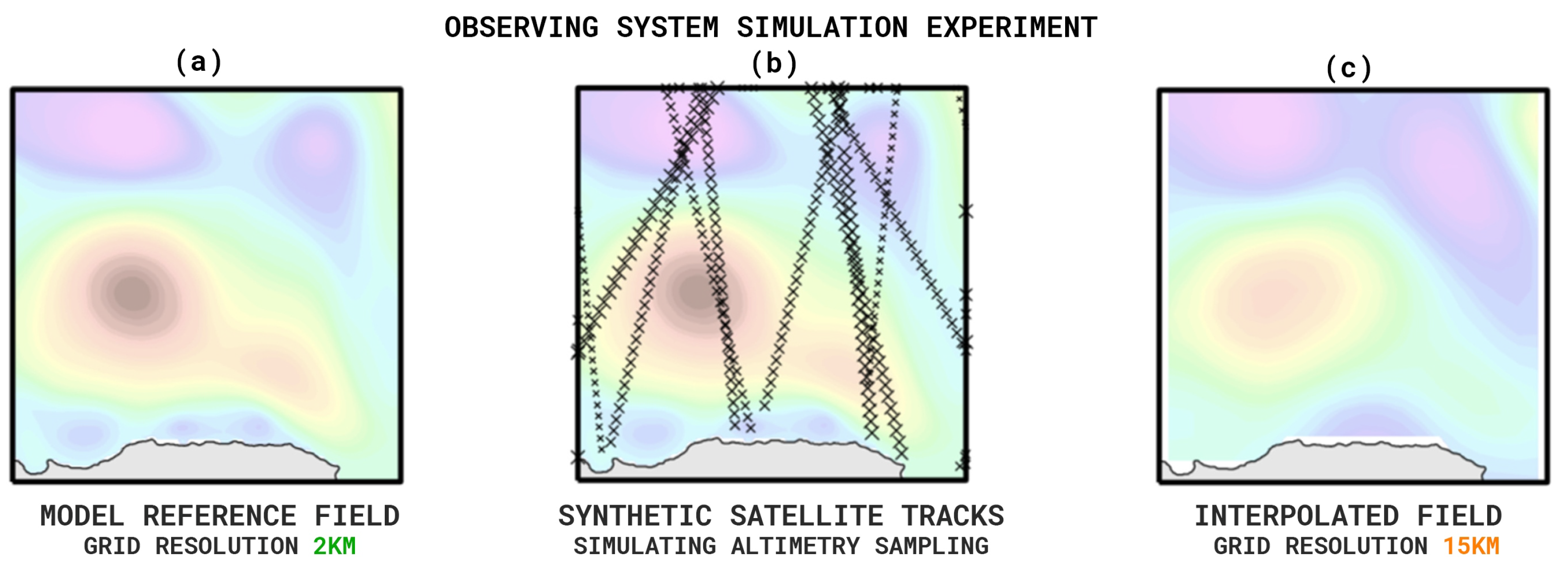
2.2. Simulated Satellite Data

Geophysical simulations of the ocean allow for us to train data-driven methods using supervised learning because we have access to sufficient quantities of ground truth labels. To train our model, we use the CROCO Numerical Model of the Ocean (http://www.croco-ocean.org), a realistic numerical simulation of ocean circulation [12]. In particular, we use simulations from the Mediterranean Sea with assimilated data from 2015 and 2016, which we split into training and validation sets, respectively. This allows for us to to capture seasonal variations both during evaluation and model training. CROCO solves fluid dynamics equations on a grid with a horizontal resolution of 2 km, providing numerous parameters including ageostrophic surface velocities (vector components U and V) as well as SSH and SST fields.

The reference ground truth of SSH provided by the CROCO model simulations, as seen in Figure 2a, needs to be downsampled in an inhomogeneous manner in order to reproduce the exact observation error found in the satellite altimetry data. An Observing System Simulation Experiment (OSSE) allows the use to imitate low-resolution SSH products using optimal interpolation methods. Synthetic satellite tracks from a four-satellite configuration are reproduced through the SWOT simulation method presented in [54], providing realistic measurement errors and noise. Figure 2b illustrates a representation of synthetic satellite tracks covering the numerical field generated by the CROCO model. The resulting synthetically observed field is then processed to compute gridded fields with the same interpolation schema that is utilized for the production of gridded AVISO/DUACS SSH satellite data [20]. It consists of an inhomogeneous spatiotemporal interpolation between the sampled points by the synthetic tracks, shown in Figure 2c. The resolution is thus downgraded from a high-resolution version of a 2 km grid size to a low-resolution version of a 15 km grid size. The high-resolution SST, the low-resolution SSH, and the corresponding geostrophic U and V are used as inputs to our model; the high-resolution SSH and ageostrophic U and V are ground truth outputs used as supervision.

The infrared observation that provides SST is unable to retrieve data under cloud coverage that is often present at the observation time, so the SST contains missing data points. Since the simulated SST data that we use for training are cloud-free, we artificially add cloud to the training image patches. We sample clouds from real L3 SST observations to ensure that the distribution of our synthetic clouds used in training follows that of real observations.

2.3. Drifter Data

To evaluate the models on real data, we use in situ measurements of sea surface currents from autonomous drifting buoys that are passively transported by the ocean surface currents. We use two years (2021–2022) of drifter observations from the Mediterranean Sea as a test set illustrated in Figure 3. To remove noise, we use a 24 h sliding window filter to smooth drifter motions. With the application of optimal ship routing in consideration, we filter our drifter test set to only observations of current magnitudes of above 0.25 m/s, as low magnitude currents have little effect on route optimization. We consider sets of observations from a particular drifter on a particular day (drifter days), which we compare to our daily current predictions. This offers us in total 2724 drifter day observations from different locations on the Mediterranean Sea. These sets of observations come from a total of 102,429 observations from a total of 112 drifters. In the pseudo-labeling stage of our method, described later in Section 2.6, we restrict this test set to 1588 drifter day observations from 2022, as we use 2021 observations during training.

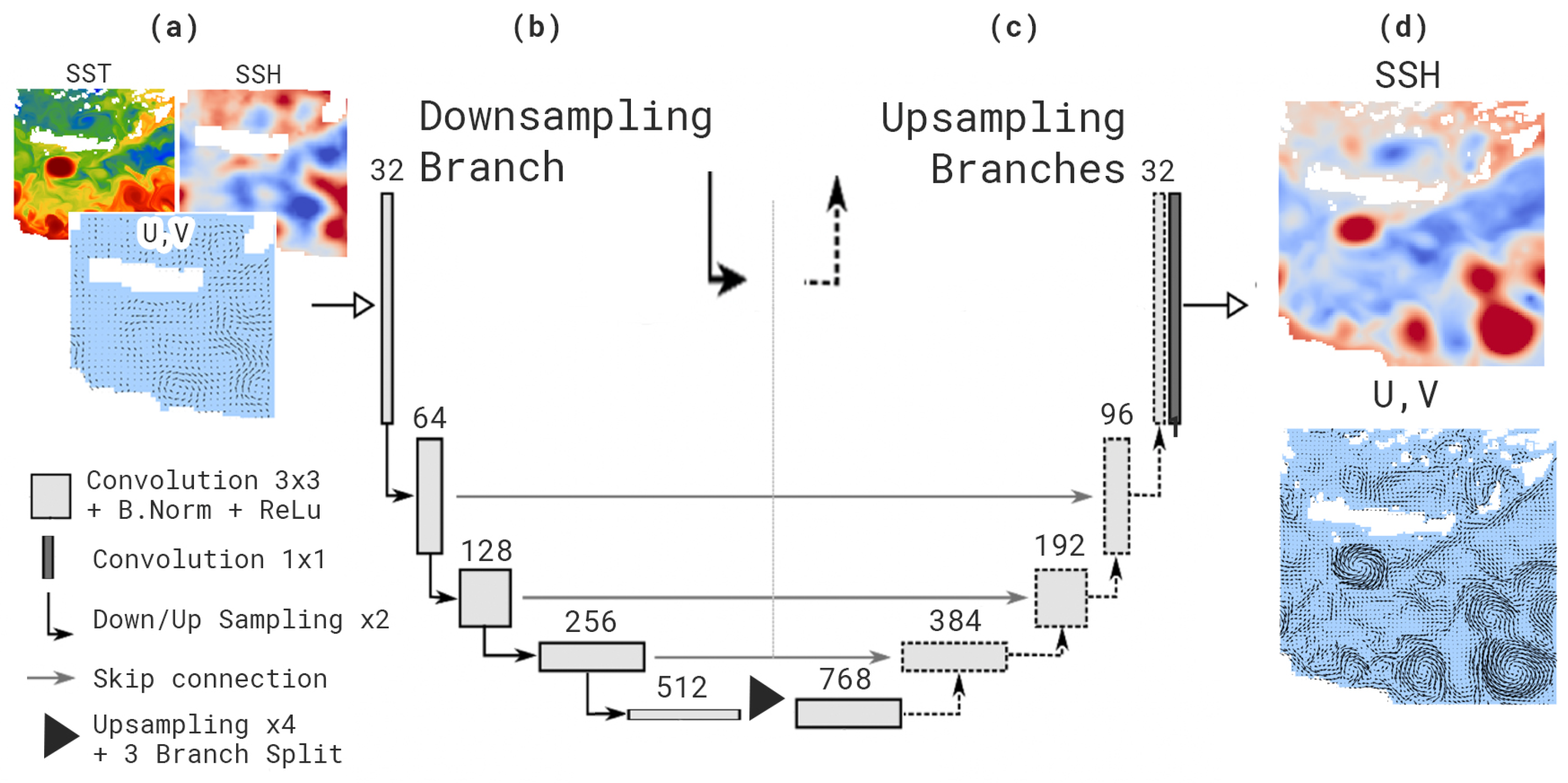
2.4. Model Architecture

Our model architecture is a U-Net encoder–decoder, specifically designed for multi-channel image-to-image problems. We refer to [28] for a detailed description of U-Net architecture. In the encoder, each block comprises two $3\times 3$ convolution operations with a ReLU activation, followed by a max-pooling layer that reduces the spatial dimension by a factor of 2. The decoder follows a similar structure, but instead of the max-pooling layer, we employ a nearest neighbor up-sampling operation. Skip connections concatenate features from the down-sampling to the up-sampling branch, enabling multi-scale spatial sampling by progressively transforming the input image size. This approach allows for us to capture ocean dynamics across various spatial scales. In [55], the authors demonstrate that batch normalization layers shrink the standard deviation of residual features, leading to performance degradation in super-resolution networks. Consequently, we opt to remove batch normalization layers.

Our primary model, called HIRES-CURRENTS-Net, takes four 2D inputs (SST, SSH, U, and V) and produces three 2D outputs (SSH, U, and V). Figure 4 provides an example of an input/output pair. Our model architecture is illustrated in Figure 5. In the traditional U-Net implementation, there is a single encoder and decoder, where the encoder and decoder may process multi-channel images. In our approach, however, the inputs are fed into the encoder as a multi-channel image, but we employ three separate single-channel decoders to produce SSH, U, and V outputs. This modification to the U-Net architecture is introduced in [56], demonstrating enhanced performance in a task of ocean eddy segmentation using similar data as shown in [30]. The rationale behind this adjustment is rooted in the distinct nature of the produced outputs (SSH, U, and V); thus, employing a single decoder for all outputs might lead to a decrease in performance. In Section 3.5, we provide ablation studies comparing the performance of a single multi-channel decoder to that of multiple decoders for each channel.

Our loss function is a weighted MSE loss computed for each of the output channels $Y\in \{\mathrm{SSH},\mathrm{U},\mathrm{V}\}$ at each pixel with index $(i,j)$ where $i\in \{1,\dots ,N\}$ and $j\in \{1,\dots ,M\}$ for an image of size $N\times M$, which in our case is $128\times 128$ pixels. Weights $w_{ij}$ are equal to 0 if the pixel is on land and are proportional to the magnitude of ground truth currents if the pixel is on water. Y denotes ground truth and $\widehat{Y}$ denotes our prediction of each output variable.

$$MS{E}_Y=\frac{1}{N\times M}\sum _{j=1}^M\sum _{i=1}^N{w}_{ij}{(Y_{ij}-{\widehat{Y}}_{ij})}^2$$

(1)

The total loss is computed as

$$MS{E}_{total}=MS{E}_{SSH}+MS{E}_U+MS{E}_V.$$

(2)

2.5. Training with Artificial Clouds

To enhance model robustness to clouds in real-time operational SST observations, we add artificial clouds to the simulated data used in training. The cloud bank is constructed by taking random crops of clouds from past SST images. The distribution of these artificial clouds thus reflects the real distribution of clouds observed in SST images. To simplify the analysis of the impact of clouds on the performance of our model, we divide cloud coverage into four categories: low (0–40%), medium (40–60%), high (60–80%), and very high (80–100%), illustrated in Figure 6.

2.6. Fine-Tuning on Real Observations

In order to reduce the possible domain gap between the simulated training data and real satellite data, we propose a novel pseudo-labeling strategy. In order to obtain high-quality pseudo-labels for real data, we input high-quality altimetric data and high-quality SST data to the model, which are not available in real-time operational settings. In real-time operational settings, our model inputs altimetric data available in real time, derived from interpolating altimetric observations from previous days. However, delayed-time altimetric interpolations are of higher quality due to additional observations from future dates. We can thus input delayed-time altimetry to our model to obtain higher-quality pseudo-labels for fine-tuning our model on real data. Also, we can consider only low-cloud SST images. In Section 3.3, we demonstrate that by using high-quality altimetric data and low-cloud SST images, we obtain very accurate predictions of currents. These pseudo-labels can then be used to fine-tune our model using inputs which are available in real time. We can also use the pseudo-labels to train the model on alternative high-resolution inputs such a chlorophyll concentration.

2.7. Evaluation Metrics

Ocean drifters provide sparse measurements of the direction and magnitude of ocean currents, allowing comparisons of our model with ground truth observational data. Our evaluation metrics are designed with real-time operational applications in mind, such as optimal ship routing.

As described in Section 2.3, our drifter evaluation set contains D = 102,429 observations from $N=2724$ unique drifter days, i.e., a set of $n_j$ observations for a particular drifter on a particular day (drifter day $j\in \{1,\dots ,N\}$, where ${\sum }_{j=1}^N{n}_j=D$). We consider two metrics: the percentage of correctly predicted angles and the percentage of correctly predicted magnitude values for our set of drifter day observations. These simple and interpretable metrics capture the frequency of correct predictions of the direction and magnitude of the force of the currents applied to a ship or another floating object in the ocean.

Equation (3) describes the angle and magnitude metrics, where $f_{\left\{\mathrm{a},\mathrm{m}\right\}}\left(d_{ij},{\widehat{d}}_{ij}\right)$ is either the absolute circular angle difference ($f_{\mathrm{a}}$) or the absolute magnitude difference ($f_{\mathrm{m}}$) between the drifter observation $d_{ij}$ and our prediction ${\widehat{d}}_{ij}$ for a single drifter observation i for drifter day j. The function $\mathbb{1}$ is the identity function, outputting 1 when the average angle or magnitude difference is below a certain threshold $T_{\left\{\mathrm{a},\mathrm{m}\right\}}$ and 0 otherwise.

$$\frac{1}{N}\sum _{j=1}^N\mathbb{1}\left(\left(\frac{1}{n_j}\sum _{i=1}^{n_j}{f}_{\left\{\mathrm{a},\mathrm{m}\right\}}\left(d_{ij},{\widehat{d}}_{ij}\right)\right)\le T_{\left\{\mathrm{a},\mathrm{m}\right\}}\right)$$

(3)

In practice, $T_{\mathrm{a}}={45}^{\circ }$ and $T_{\mathrm{m}}=0.15$ m/s. As low-magnitude currents do not have a strong impact on ships, we consider only drifter observations which measure currents of over $0.25$ m/s during evaluation, and the average magnitude of currents measured by drifters in our test set is $0.3$ m/s. The threshold of $0.15$ m/s thus corresponds to an around 50% error in current magnitudes.

2.8. Comparison to Baselines

We compare to two commonly used baselines: Mercator and AVISO/DUACS optimal interpolation. The Mercator baseline uses the Mercator-Ocean [10] assimilated geophysical model, available in real time. The AVISO/DUACS baseline is a daily AVISO/DUACS [20] multimission altimeter product providing real-time gridded geostrophic U and V components of ocean surface currents using optimal interpolation.

2.9. Implementation Details

When training on simulated data, we employ a learning rate of ${10}^{-4}$ and conduct training over 100,000 random crops of the Mediterranean Sea. This number of random crops was chosen by evaluating our model on a small subset of drifters, which are not included in our test set. We find that when we train our model on additional random samples, it tends to overfit to the simulated data and generalizes less well to the real data.

We use an Adam optimizer with a weight decay parameter of ${10}^{-3}$. The image pixel size is set to $128\times 128$, and a batch size of 16 is utilized. Each channel of every input image undergoes normalization based on the mean and standard deviation of the respective image. This alleviates systematic biases which may be present between the simulated data used during training and the real satellite observations which are used during evaluation. Throughout training, the output high-resolution predictions of SSH, U, and V are normalized using the per-image means and standard deviations of the input low-resolution SSH, U, and V, respectively.

The crops are randomly selected from the training area area, and only those containing at least $50\%$ of the crop size of non-missing values related to the land are retained. Land values are excluded from the loss function calculation, and we proportionally weight the loss by the magnitude of the current, as detailed in Section 2.4. Cloud areas are masked with a constant out-of-distribution value across all patches with artificial clouds.

3. Results

In this section, we present our experimental results when training on simulated data (Section 3.1), training using artificial clouds (Section 3.2), and training using pseudo-labels on real data (Section 3.3). We also show qualitative results (Section 3.4) and provide supplementary justifications of our choice of model architecture with ablation studies (Section 3.5).

3.1. Training on Simulated Data

We train our model using cloud-free SST, low-resolution SSH, U, and V from the CROCO OSSE as inputs, the simulated high-resolution ground truth values of SSH, and ageostrophic U and V (velocity field of currents). During the evaluation on real data, we use cloud-free interpolated L4 SST as an input. Our HIRES-CURRENTS-Net model (HIRES-CUR) achieves better performance than the commonly used methods of real-time operational estimates of ocean currents, according to our evaluation strategy on real drifter observations, as shown in Table 1. HIRES-CURRENTS-Net correctly predicts the angles of the currents measured by drifters 72% of the time, while Mercator correctly predicts 52% of the angles measured by drifters and AVISO/DUACS correctly predicts 68% of the currents measured by drifters. Our model also obtains 46% of correct magnitude predictions—a significant boost compared to AVISO/DUACS (39%) and Mercator (33%). As AVISO/DUACS is a stronger baseline than Mercator, we compare our models with AVISO/DUACS in future evaluations for simplicity.

Table 1. Performance comparison of the standard methods (Mercator and AVISO/DUACS) and our model HIRES-CUR. We evaluate the results on the drifter test set with high (>0.25 m/s) magnitudes based on two evaluation metrics: correct angles percentage described in Equation (3) and illustrated in Figure 7 and correct magnitude percentage described in Equation (3). The threshold to define the correct angle prediction is chosen as angle error $\theta <$ 45°. The threshold to define the correct magnitude prediction is chosen as absolute magnitude error $|\Delta M|<$ 0.15 m/s. HIRES-CUR outperforms common methods of real-time operational predictions of ocean currents, such as AVISO/DUACS and Mercator. Best results are in bold font.

Model	Correct Angles, %	Correct Magnitudes, %
Mercator	50.26	32.56
AVISO/DUACS	67.86	38.57
HIRES-CUR	71.73	45.73

Table 1. Performance comparison of the standard methods (Mercator and AVISO/DUACS) and our model HIRES-CUR. We evaluate the results on the drifter test set with high (>0.25 m/s) magnitudes based on two evaluation metrics: correct angles percentage described in Equation (3) and illustrated in Figure 7 and correct magnitude percentage described in Equation (3). The threshold to define the correct angle prediction is chosen as angle error $\theta <$ 45°. The threshold to define the correct magnitude prediction is chosen as absolute magnitude error $|\Delta M|<$ 0.15 m/s. HIRES-CUR outperforms common methods of real-time operational predictions of ocean currents, such as AVISO/DUACS and Mercator. Best results are in bold font.

Model	Correct Angles, %	Correct Magnitudes, %
Mercator	50.26	32.56
AVISO/DUACS	67.86	38.57
HIRES-CUR	71.73	45.73

Whilst optimal interpolation reconstructs currents from sparse altimetry observations, our HIRES-CURRENTS-Net model additionally has access to high-resolution information from SST images.

Table 2. Performance comparison of standard method AVISO/DUACS and our model trained using SST as an extra input channel (HIRES-CUR) and without SST as an input (HIRES-CUR w/o SST) based on the evaluation metrics described in Table 1. Evaluation is performed only on currents with high (>0.25 m/s) magnitudes. The boost in correctly predicted angles when using HIRES-CUR with respect to AVISO/DUACS comes from the high-resolution SST inputs, with visible signatures of ocean surface currents. Best results are in bold font.

Model	Correct Angles, %	Correct Magnitudes, %
AVISO/DUACS	67.86	38.57
HIRES-CUR w/o SST	66.56	43.50
HIRES-CUR	71.73	45.73

presents a comparison between HIRES-CURRENTS-Net trained with and without SST as an input, demonstrating that high-resolution SST information is required to provide a significant boost.

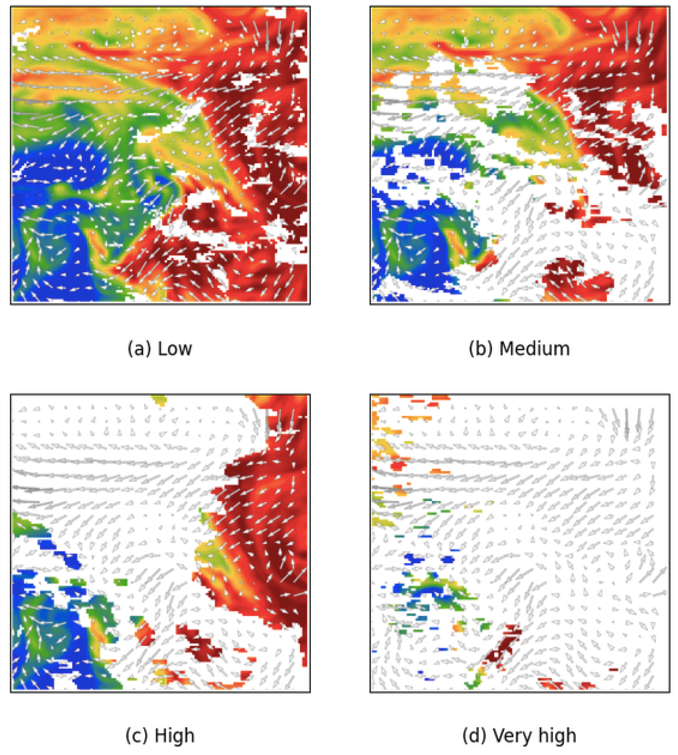
3.2. Cloud Robustness

One likely source of performance degradation in our model is the presence of clouds, which obstructs the observation of SST. In order to increase the robustness of our model when the SST data are inaccurate or missing, we train the model using artificial clouds.

Table 3. Performance comparison of our model trained on simulated satellite data with synthetic clouds (HIRES-CUR-cloud) and without synthetic clouds (HIRES-CUR) on the input SST images. The models are evaluated on the drifter test set with high (>0.25 m/s) magnitudes using both L3 and L4 SST products as inputs. The evaluation metrics are described in Table 1. By incorporating artificial clouds during training, we slightly boost the performance of HIRES on the L4 SST (from 71.73% to 73.20%) and obtain a significant boost in performance for the L3 SST (from 61.23% to 72.47%), demonstrating that we can apply the model to L3 SST data instead of L4 SST data with only a minor loss in performance. Best results are in bold font.

Input	Model	Correct Angles, %	Correct Magnitudes, %
L4 SST	HIRES-CUR	71.73	45.73
	HIRES-CUR-cloud	73.20	48.13
L3 SST	HIRES-CUR	61.23	40.23
	HIRES-CUR-cloud	72.47	48.17

shows that incorporating artificial clouds during training offers a boost in performance on drifters, increasing the percentage of correct angles from 72% to 73% and the percentage of correct magnitudes from 44% to 46%.

Moreover, training the model using artificial clouds allows for us to apply the model to L3 SST data, where pixels with clouds are missing, unlike L4 SST data which requires an additional processing step to interpolate over cloudy pixels. Table 3 shows that when trained using clouds and applied to L3 SST data, HIRES still performs well, with 72% correctly predicted angles, in comparison to the same model applied to L4 SST data, which achieves 73% correctly predicted angles. In both cases, our model achieves 48% correctly predicted magnitudes. When HIRES is not trained using artificial clouds, the model performs poorly. This is expected as the model does not see missing pixels during training.

The performance of our model is impacted by cloud cover.

Table 4. Performance comparison of standard method AVISO/DUACS and our models trained with synthetic clouds (HIRES-CUR-cloud) and without synthetic clouds (HIRES-CUR) on the SST images, evaluated on the drifter test set with high (>0.25 m/s) magnitudes on each of the four categories of the cloud cover. The evaluation metrics are described in Table 1. Errors in HIRES-CUR predictions are correlated with cloud coverage, but training our model using synthetic clouds offers a performance boost, particularly in areas with medium to very high cloud coverage. Best results are in bold font.

% Clouds	Model	Correct Ang., %	Correct Mag., %	# Drifter-Days
≥80% (very high)	AVISO/DUACS	62.28	32.70	896
	HIRES-CUR	62.31	35.27
	HIRES-CUR-cloud	65.18	41.18
60–80% (high)	AVISO/DUACS	66.43	38.52	283
	HIRES-CUR	68.94	44.52
	HIRES-CUR-cloud	71.02	48.76
40–60% (medium)	AVISO/DUACS	67.66	40.26	303
	HIRES-CUR	69.33	46.86
	HIRES-CUR-cloud	75.25	53.14
<40% (low)	AVISO/DUACS	72.57	42.73	1163
	HIRES-CUR	80.49	53.83
	HIRES-CUR-cloud	79.19	52.02

decomposes the evaluation metrics by percentage of cloud cover for the baseline model AVISO/DUACS, for HIRES-CURRENTS-Net trained without artificial clouds (HIRES-CUR), and for HIRES-CURRENTS-Net trained with artificial clouds (HIRES-CUR-cloud). The model is applied to L4 SST inputs for fair comparison between HIRES-CUR and HIRES-CUR-cloud.

Our model outperforms AVISO/DUACS even when cloud cover is high. However, as expected, the error of our model is correlated with the percentage of clouds present in the SST image. The percentage of correct angles when HIRES-CURRENTS-Net is trained without clouds is 65–66% when there are 80–100% of clouds in the SST image but is 79–80% when there are 0–40% of clouds in the SST image. When there are 80–100% of clouds in the SST image, the percentage of correct magnitudes is 35% when HIRES-CURRENTS-Net is trained without clouds and 41% when HIRES-CURRENTS-Net is trained with clouds. When there are less than 40% of clouds in the SST image, the percentage of correct magnitudes is 54% when HIRES-CURRENTS-Net is trained without clouds and 52% when HIRES-CURRENTS-Net is trained with clouds. The performance boost due to training on artificial clouds is particularly significant in areas with very high to medium cloud coverage, increasing the percentage of correctly predicted angles from 62% to 65% for areas with very high cloud coverage, from 69% to 71% for high cloud coverage, and from 69% to 75% when there is medium cloud coverage.

We note that the error of AVISO/DUACS is also correlated with the percentage of clouds due to the seasonal stratification effect, where the upper layers of the ocean during winter are well mixed and ocean dynamics are more difficult to observe by altimeter observations.

3.3. Training on Real Data

To decrease the domain gap between training on simulated data and applying our model in real-time operational contexts, we apply a pseudo-labeling strategy to train our model on high-quality labels on real data. To acquire these labels, we apply our model to input data in areas with 0–40% cloud coverage and delayed-time altimetry data, which is of better quality than data available in real time.

Table 5. Performance of the HIRES-CUR model on the drifter test set with high (>0.25 m/s) magnitudes and low (<40%) cloud cover given the real-time and delayed-time altimetry as inputs. The evaluation metrics are described in Table 1. When applied to delayed-time altimetric data, our model predicts the correct angle for 81.33% of observations, and the correct magnitude for 56% of observations with the low cloud cover. These high-quality labels can then be used to fine-tune or train models using real data and inputs available in real time. Best results are in bold font.

% Clouds	Model	Input	Correct Ang., %	Correct Mag., %
<40% (low)	HIRES-CUR	Real-time	80.49	53.83
		Delayed-time	81.33	56.00

compares results on drifters for the HIRES-CURRENTS-Net model applied to low-cloud areas using both real-time and delayed-time altimetry inputs. When using delayed-time inputs in low-cloud areas, our model predicts the correct angle of drifter motion for 81% of observations and the correct magnitude for 56% of observations.

The HIRES-CUR-ftune model is trained on OSSE data from CROCO and fine-tuned using pseudo-labels from our most accurate predictions.

Table 6. Performance comparison of the standard method (AVISO/DUACS) and our models trained with synthetic clouds (HIRES-CUR-cloud) and then fine-tuned using pseudo-labels (HIRES-CUR-ftune) on the drifter test set with high (>0.25 m/s) magnitudes on both L3 and L4 SST data. The evaluation metrics are described in Table 1. By fine-tuning the model on real data with pseudo-labels, we increase the number of correctly predicted angles from 72% to 73% for both L4 SST and L3 SST inputs. However, the magnitude performance decreases after fine-tuning. Best results are in bold font.

Input	Model	Fine-Tuning	Correct Ang., %	Correct Mag., %
-	AVISO/DUACS	-	65.22	33.10
L4 SST	HIRES-CUR-cloud	None	72.23	43.07
	HIRES-CUR-ftune	Real	73.32	41.32
L3 SST	HIRES-CUR-cloud	None	72.29	44.04
	HIRES-CUR-ftune	Real	73.30	41.58

shows the results on correct angle and magnitude predictions for the real data pipeline. By fine-tuning our model on pseudo-labels, we obtain a small boost in performance when using L4 SST inputs. When using L3 SST inputs, we obtain a small boost in the percentage of correctly predicted angles, but also a slight decrease in the percentage of correctly predicted magnitudes.

Furthermore, our pseudo-labels allow for us to train our model using data which are not available in the geophysical simulation used for training, such as chlorophyll concentration.

Table 7. Performance comparison of the standard method (AVISO/DUACS) and our model trained from scratch employing pseudo-labels (HIRES-CUR-real) using L3 SST and L3 chlorophyll data as an extra input channel on the drifter test set with high (>0.25 m/s) magnitudes. The evaluation metrics are described in Table 1. Our pseudo-labeling strategy allows for us to train models from scratch on real data and alternative inputs such as chlorophyll. The performance of the model trained from scratch is slightly lower than the performance of the models pre-trained on simulated data (see Table 6), but it is still strong. Best results are in bold font.

Input	Model	Pre-Train	Correct Ang., %	Correct Mag., %
-	AVISO/DUACS	-	65.22	33.10
L3 SST	HIRES-CUR-real	None	70.34	43.95
L3 CHL	HIRES-CUR-real	None	69.90	42.00

illustrates how we can train our model from scratch using either SST data or chlorophyll concentration. Although the model trained from scratch on real data using pseudo-labels does not perform as well as the model trained on simulated data (HIRES-CUR-cloud) and the model fine-tuned on real data (HIRES-CUR-ftune), shown in Table 6, performance is still strong and significantly better than that of AVISO/DUACS.

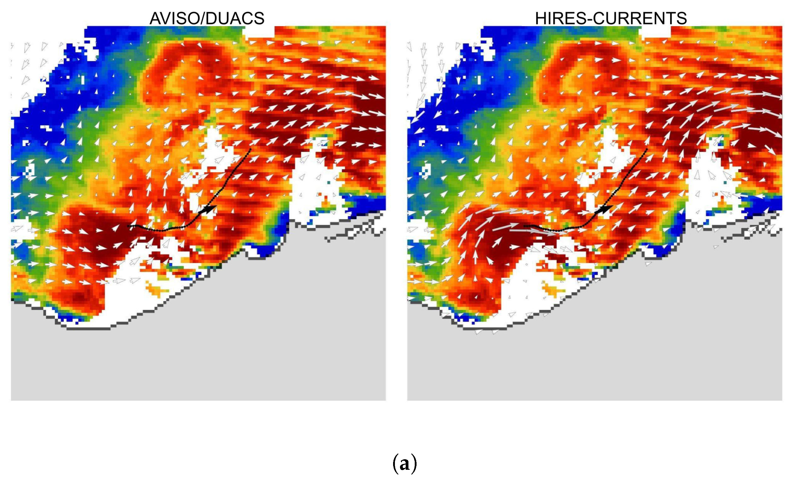
3.4. Qualitative Results

Our HIRES-CURRENTS-Net model is able to better localize fast-moving structures or better capture small-scale structures which are visible in the SST signal but which are missed by standard methods of altimetric interpolation of sparse altimetric tracks. Figure 8 shows that interpolated altimetric data (AVISO/DUACS) can incorrectly localize fast-moving or under-sampled structures, whilst our HIRES-CURRENTS-Net model detects small structures from the high-resolution SST signature. Moreover, we notice that HIRES-CURRENTS-Net tends to increase the magnitudes of fast-moving structures. This potentially contributes to the higher accuracy of predicted magnitudes on drifters, as shown in Table 1.

Figure 9 provides visualizations of velocity field predictions superimposed on SST input images in areas surrounding drifter observations. These examples further illustrate fine-scale structures captured by our model and omitted by AVISO/DUACS. In Figure 9b, a pair of small eddies is not resolved by AVISO/DUACS but is captured by HIRES-CURRENTS-Net, allowing for the model to accurately reconstruct the direction of currents around the drifter observation. Figure 9c shows an example of SST input partially obscured by clouds. Despite the missing data, our model predicts currents that align with the observed direction of the drifter.

In Figure 10, we provide a visualization of the vorticity field predicted by AVISO/DUACS and predicted by HIRES-CURRENTS-Net on CROCO-simulated data from the validation set. These examples clearly illustrate the capacity of HIRES-CURRENTS-Net to learn fine-scale structures present in the ground truth.

3.5. Further Ablations and Results

In this section, we present further ablation studies and results. We show results with and without using SSH as an input (low resolution) and as an output variable (high resolution). We also present results using a single decoder or multiple decoders in our U-Net architecture. Finally, we show that the model from Table 1 also outperforms AVISO/DUACS on the CROCO-simulated data.

Using SSH as input/output: Although our evaluation metrics only compare the angle and magnitude of predicted currents with respect to drifter observations, we also output high-resolution SSH predictions.

Table 8. Performance comparison of our model trained with SSH as an input (HIRES-CUR) and without SSH as an input (HIRES-CUR w/o SSH) based on the evaluation metrics described in Table 1. Evaluation is performed only on currents with high (>0.25 m/s) magnitudes. The performance of our model on drifters improves when including additional variable SSH as an input (low resolution) and as an output (high resolution). The results show that including SSH slightly improves angle accuracy and significantly improves magnitude accuracy. Best results are in bold font.

Model	Correct Angles, %	Correct Magnitudes, %
HIRES-CUR w/o SSH	71.18	39.65
HIRES-CUR	71.73	45.73

compares our results when using low-resolution SSH as an input or as an output, showing that performance on predicting the angle and magnitude of currents is better when including this additional variable both as a low-resolution input and a high-resolution output.

Impact of single/multiple decoders: 

Table 9. Performance comparison of the HIRES-CUR model with a single or multiple decoders based on the evaluation metrics described in Table 1 applied to our drifter test set. Evaluation is performed only on currents with high (>0.25 m/s) magnitudes. Our model with 3 decoders achieves better results when predicting angles and magnitudes than our model with 1 decoder. Best results are in bold font.

# Decoders	Model	Correct Angles, %	Correct Magnitudes, %
1	HIRES-CUR	69.13	45.30
3	HIRES-CUR	71.73	45.73

shows the impact of having a single or multiple decoders. Having three separate decoders rather than a single decoder helps the model achieve greater accuracy when predicting the angle and magnitude of drifters.

Evaluation on CROCO: 

Table 10. Performance comparison of the standard method (AVISO/DUACS) and our model (HIRES-CUR) on the validation set of the simulated satellite data obtained from the CROCO model. Here, the metrics are the average pixel-wise angle error and the average pixel-wise magnitude error for currents about 0.25 m/s when compared to the simulated ground truth values. Our HIRES model outperforms the baseline optimal interpolation method and better predicts both current angles and magnitudes. Best results are in bold font.

Model	Average Angle Error, Degrees	Average Magnitude Error, m/s
AVISO/DUACS	38.61	0.16
HIRES-CUR	26.87	0.12

shows the results of evaluating our model on the CROCO validation set. The evaluation metrics here are the average absolute angle difference and the average absolute magnitude difference between our predictions of the ocean currents and the ground truth from the simulation, filtered to ground truth magnitude values of above $0.25$ m/s. We find that our model outperforms the baseline optimal interpolation method and better predicts both the angle and the magnitude of ocean currents.

4. Discussion

In this study, we developed a real-time operational model to predict daily now-casts of ocean currents based on the fusion of multiple satellite observations: satellite altimetry data alongside high-resolution infrared images of sea surface temperature or visible images of surface chlorophyll. This fusion of different satellite observations having distinct spatial resolution is possible due to recent advances in computer vision. Evaluation on in situ measurements from drifters showed that the performance of our CNN model is superior to other commonly used alternative methods. Using qualitative examples, we illustrated that our model is capable of detecting sub-mesoscale structures which cannot be detected on standard AVISO/DUACS products. Although new generations of wide-swath altimeters (SWOTs) can resolve sub-mesoscale dynamics [2], it will take many years to deploy a constellation of SWOT satellites able to map the global ocean in real time. Hence, in the near future, the spatial resolution of real-time observations of surface geostrophic currents is still restricted by spatio-temporal interpolation of the nadir altimeters. In comparison, the fusion of multiple satellite observations using computer vision provides a reliable reconstruction of surface currents at high resolution to capture both mesoscale and sub-mesoscale features.

A similar approach using the Observing System Simulation Experiment to train a deep learning model was performed by Nardelli et al. [53] to describe the sea surface height at high resolution. However, we can only retrieve the geostrophic currents from the SSH field, while our approach targets the full surface velocity, including cyclostrophic components. The other key difference is that our model is robust to partial cloud coverage and can be applied both on L4 or L3 SST data, with little difference in performance. Furthermore, we introduce a novel pseudo-labeling strategy, allowing for our model to be fine-tuned on real data to reduce the domain gap between real and simulated data. We demonstrated that our model can also be trained from scratch using alternative inputs such as chlorophyll.

Another noteworthy extension of our work is the proposition of a quantitative comparison with in situ data using specifics metrics focused on strong currents that have a significant impact on horizontal advection or the speed over ground of large cargos. Figure 11 represents the comparison between a reference drifter database and our HIRES-CURRENTS-Net model and two standard methods, MERCATOR and AVISO/DUACS in terms of angle error for different thresholds (see Figure 7). The plot shows that in terms of surface current direction, our model substantially outperforms both algorithms for the given angle thresholding strategies.

Our HIRES-CURRENTS-Net model is fully operational for short-term optimal routing of ships. With high-resolution predictions of ocean currents, it is possible to compute optimal trajectories between two sea ports in order to save time and fuel by following favorable currents. As illustrated in Figure 12, a roll-on/roll-off cargo ship traveling along the Algerian coast in November 2023 benefited from this approach. Initially, its path was hindered by several coastal eddies, which can be accurately located using our method. We use isochrone methods to compute waypoints to propose an optimal route, which we propose one day in advance using available near real-time satellite data. With our short-term optimization, the vessel altered its course slightly northward, circumventing the eddies. This minor detour allowed for the ship to save over an hour on this journey and cut fuel consumption. The impact of the surface currents can be computed by subtracting measurements of Speed Through Water (STW) from onboard instruments from Speed Over Ground (SOG) measured by the ship’s automatic identification system (AIS), as shown in Figure 12b. Optimizing ship routes leads to reduced travel time and fuel savings. This approach can significantly cut shipping costs and lower carbon emissions, contributing to sustainability by minimizing the environmental impact of shipping activities.

For longer voyages, reliable forecasts of surface currents are required around one week in advance. In further work, a time dimension could be included in our model to process a time series of multiple satellite observations and output an accurate operational forecast of ocean currents.

5. Conclusions

HIRES-CURRENTS-Net is an operational solution for producing daily now-casts of ocean currents in the Mediterranean Sea from satellite data inputs available in near real time, in particular sea surface height, sea surface temperature, and cholorophyll. One application of our method is the optimization of ship routes to save time and fuel costs, as well as reduction in carbon emissions. Our model is capable of predicting small and fast-moving structures missed by altimetric observations and achieves significantly better performance than other commonly used operational methods for producing now-casts of ocean currents. Our model is evaluated using in situ data from the Mediterranean Sea, but further work is needed to fine-tune our model and evaluate performance in other regions. Forecasting ocean currents is necessary for longer ship routes which may last one or two weeks, and our model could be extended to predict multiple time steps in the future.

References

1. Fu, L.; Cazenave, A. Satellite Altimetry and Earth Sciences: A Handbook of Techniques and Applications; International Geophysics Series; Academic Press: Cambridge, MA, USA, 2001. [Google Scholar]
2. Morrow, R.; Fu, L.L.; Ardhuin, F.; Benkiran, M.; Chapron, B.; Cosme, E.; d’Ovidio, F.; Farrar, J.T.; Gille, S.T.; Lapeyre, G.; et al. Global Observations of Fine-Scale Ocean Surface Topography With the Surface Water and Ocean Topography (SWOT) Mission. Front. Mar. Sci. 2019, 6, 232. [Google Scholar] [CrossRef]
3. Amores, A.; Jordà, G.; Arsouze, T.; Le Sommer, J. Up to What Extent Can We Characterize Ocean Eddies Using Present-Day Gridded Altimetric Products? J. Geophys. Res. Ocean. 2018, 123, 7220–7236. [Google Scholar] [CrossRef]
4. Stegner, A.; Le Vu, B.; Dumas, F.; Ghannami, M.A.; Nicolle, A.; Durand, C.; Faugere, Y. Cyclone-Anticyclone Asymmetry of Eddy Detection on Gridded Altimetry Product in the Mediterranean Sea. J. Geophys. Res. Ocean. 2021, 126, e2021JC017475. [Google Scholar] [CrossRef]
5. Ioannou, A.; Moschos, E.; Le Vu, B.; Stegner, A. Short-Term Optimal Ship Routing via Reliable Satellite Current Data. In Proceedings of the NAME International Symposium on Ship Operations, Management and Economics, Athens, Greece, 7–8 March 2023. [Google Scholar] [CrossRef]
6. Dong, C.; Xu, G.; Han, G.; Bethel, B.J.; Xie, W.; Zhou, S. Recent Developments in Artificial Intelligence in Oceanography. Ocean-Land Res. 2022, 2022, 9870950. [Google Scholar] [CrossRef]
7. Buongiorno Nardelli, B.; Cavaliere, D.; Charles, E.; Ciani, D. Super-Resolving Ocean Dynamics from Space with Computer Vision Algorithms. Remote Sens. 2022, 14, 1159. [Google Scholar] [CrossRef]
8. Fablet, R.; Febvre, Q.; Chapron, B. Multimodal 4DVarNets for the reconstruction of sea surface dynamics from SST-SSH synergies. IEEE Trans. Geosci. Remote Sens. 2023, 61, 4204214. [Google Scholar] [CrossRef]
9. Sommer, J.; Chassignet, E.; Wallcraft, A. Ocean Circulation Modeling for Operational Oceanography: Current Status and Future Challenges. In New Frontiers in Operational Oceanography; Chassignet, E.P., Pascual, A., Tintore, J., Verron, J., Eds.; GODAE OceanView, 2018; pp. 289–308. [Google Scholar] [CrossRef]
10. Drévillon, M.; Bourdallé-Badie, R.; Derval, C.; Lellouche, J.; Rémy, E.; Tranchant, B.; Benkiran, M.; Greiner, E.; Guinehut, S.; Verbrugge, N.; et al. The GODAE/Mercator-Ocean global ocean forecasting system: Results, applications and prospects. J. Oper. Oceanogr. 2008, 1, 51–57. [Google Scholar] [CrossRef]
11. Lellouche, J.M.; Greiner, E.; Le Galloudec, O.; Garric, G.; Regnier, C.; Drevillon, M.; Benkiran, M.; Testut, C.E.; Bourdalle-Badie, R.; Gasparin, F.; et al. Recent updates to the Copernicus Marine Service global ocean monitoring and forecasting real-time 1/12 high-resolution system. Ocean Sci. 2018, 14, 1093–1126. [Google Scholar] [CrossRef]
12. Jullien, S.; Caillaud, M.; Benshila, R.; Bordois, L.; Cambon, G.; Dumas, F.; Gentil, S.L.; Lemarié, F.; Marchesiello, P.; Theetten, S.; et al. CROCO Technical and Numerical Documentation. Zenodo 2022. Technical Note. [Google Scholar] [CrossRef]
13. Brodeau, L.; Sommer, J.L.; Albert, A. Ocean-next/eNATL60: Material describing the set-up and the assessment of NEMO-eNATL60 simulations. Zenodo 2020. Technical Note. [Google Scholar] [CrossRef]
14. Castillo, J.M.; Lewis, H.W.; Mishra, A.; Mitra, A.; Polton, J.; Brereton, A.; Saulter, A.; Arnold, A.; Berthou, S.; Clark, D.; et al. The Regional Coupled Suite (RCS-IND1): Application of a flexible regional coupled modelling framework to the Indian region at kilometre scale. Geosci. Model Dev. 2022, 15, 4193–4223. [Google Scholar] [CrossRef]
15. Chelton, D.B.; Ries, J.C.; Haines, B.J.; Fu, L.L.; Callahan, P.S. Satellite altimetry. In International Geophysics; Elsevier: Amsterdam, The Netherlands, 2001; Volume 69, pp. i–ii. [Google Scholar]
16. Nerem, R.S.; Chambers, D.P.; Choe, C.; Mitchum, G.T. Estimating mean sea level change from the TOPEX and Jason altimeter missions. Mar. Geod. 2010, 33, 435–446. [Google Scholar] [CrossRef]
17. Abdalla, S.; Kolahchi, A.A.; Ablain, M.; Adusumilli, S.; Bhowmick, S.A.; Alou-Font, E.; Amarouche, L.; Andersen, O.B.; Antich, H.; Aouf, L.; et al. Altimetry for the future: Building on 25 years of progress. Adv. Space Res. 2021, 68, 319–363. [Google Scholar] [CrossRef]
18. Evensen, G. Data Assimilation: The Ensemble Kalman Filter; Springer: Berlin/Heidelberg, Germany, 2009; Volume 2. [Google Scholar]
19. Cressie, N. Statistics for Spatial Data; John Wiley & Sons: Hoboken, NJ, USA, 2015. [Google Scholar]
20. Taburet, G.; Sanchez-Roman, A.; Ballarotta, M.; Pujol, M.I.; Legeais, J.F.; Fournier, F.; Faugere, Y.; Dibarboure, G. DUACS DT2018: 25 years of reprocessed sea level altimetry products. Ocean Sci. 2019, 15, 1207–1224. [Google Scholar] [CrossRef]
21. Benkiran, M.; Ruggiero, G.; Greiner, E.; Le Traon, P.Y.; Rémy, E.; Lellouche, J.M.; Bourdallé-Badie, R.; Drillet, Y.; Tchonang, B. Assessing the impact of the assimilation of swot observations in a global high-resolution analysis and forecasting system part 1: Methods. Front. Mar. Sci. 2021, 8, 691955. [Google Scholar] [CrossRef]
22. Biancamaria, S.; Lettenmaier, D.P.; Pavelsky, T.M. The SWOT mission and its capabilities for land hydrology. Remote Sens. Water Resour. 2016, 55, 117–147. [Google Scholar]
23. LeCun, Y.; Bengio, Y.; Hinton, G. Deep learning. Nature 2015, 521, 436–444. [Google Scholar] [CrossRef]
24. Goodfellow, I.; Bengio, Y.; Courville, A. Deep Learning; MIT Press: Cambridge, MA, USA, 2016. [Google Scholar]
25. Li, Z.; Yang, W.; Peng, S.; Liu, F. A Survey of Convolutional Neural Networks: Analysis, Applications, and Prospects. arXiv 2020, arXiv:2004.02806. [Google Scholar] [CrossRef]
26. Dong, C.; Loy, C.C.; He, K.; Tang, X. Image super-resolution using deep convolutional networks. IEEE Trans. Pattern Anal. Mach. Intell. 2015, 38, 295–307. [Google Scholar] [CrossRef]
27. Yamanaka, J.; Kuwashima, S.; Kurita, T. Fast and accurate image super resolution by deep CNN with skip connection and network in network. In Proceedings of the Neural Information Processing: 24th International Conference—ICONIP 2017, Guangzhou, China, 14–18 November 2017; Proceedings, Part II 24. Springer: Berlin/Heidelberg, Germany, 2017; pp. 217–225. [Google Scholar]
28. Ronneberger, O.; Fischer, P.; Brox, T. U-net: Convolutional networks for biomedical image segmentation. In Proceedings of the Medical Image Computing and Computer-Assisted Intervention—MICCAI 2015: 18th International Conference, Munich, Germany, 5–9 October 2015; Proceedings, Part III 18P. Springer: Berlin/Heidelberg, Germany, 2015; pp. 234–241. [Google Scholar]
29. Moschos, E.; Stegner, A.; Le Vu, B.; Schwander, O. Real-Time Validation of Operational Ocean Models Via Eddy-Decting Deep Neural Networks. In Proceedings of the IGARSS 2022–2022 IEEE International Geoscience and Remote Sensing Symposium, Kuala Lumpur, Malaysia, 17–22 July 2022; IEEE: Piscataway, NJ, USA, 2022; pp. 8008–8011. [Google Scholar]
30. Moschos, E.; Kugusheva, A.; Coste, P.; Stegner, A. Computer Vision for Ocean Eddy Detection in Infrared Imagery. In Proceedings of the IEEE/CVF Winter Conference on Applications of Computer Vision, Waikoloa, HI, USA, 2–7 January 2023; pp. 6395–6404. [Google Scholar]
31. Zhao, N.; Huang, B.; Yang, J.; Radenkovic, M.; Chen, G. Oceanic Eddy Identification Using Pyramid Split Attention U-Net With Remote Sensing Imagery. IEEE Geosci. Remote Sens. Lett. 2023, 20, 1500605. [Google Scholar] [CrossRef]
32. Kim, S.M.; Shin, J.; Baek, S.; Ryu, J.H. U-Net convolutional neural network model for deep red tide learning using GOCI. J. Coast. Res. 2019, 90, 302–309. [Google Scholar] [CrossRef]
33. Gao, L.; Li, X.; Kong, F.; Yu, R.; Guo, Y.; Ren, Y. AlgaeNet: A deep-learning framework to detect floating green algae from optical and SAR imagery. IEEE J. Sel. Top. Appl. Earth Obs. Remote Sens. 2022, 15, 2782–2796. [Google Scholar] [CrossRef]
34. Radhakrishnan, K.; Scott, K.A.; Clausi, D.A. Sea ice concentration estimation: Using passive microwave and SAR data with a U-net and curriculum learning. IEEE J. Sel. Top. Appl. Earth Obs. Remote Sens. 2021, 14, 5339–5351. [Google Scholar] [CrossRef]
35. Ren, Y.; Li, X.; Yang, X.; Xu, H. Development of a dual-attention U-Net model for sea ice and open water classification on SAR images. IEEE Geosci. Remote Sens. Lett. 2021, 19, 4010205. [Google Scholar] [CrossRef]
36. Saharia, C.; Ho, J.; Chan, W.; Salimans, T.; Fleet, D.J.; Norouzi, M. Image super-resolution via iterative refinement. IEEE Trans. Pattern Anal. Mach. Intell. 2022, 45, 4713–4726. [Google Scholar] [CrossRef]
37. Ajayi, A.; Le Sommer, J.; Chassignet, E.; Molines, J.M.; Xu, X.; Albert, A.; Cosme, E. Spatial and temporal variability of the North Atlantic eddy field from two kilometric-resolution ocean models. J. Geophys. Res. Ocean. 2020, 125, e2019JC015827. [Google Scholar] [CrossRef]
38. Ciani, D.; Charles, E.; Buongiorno Nardelli, B.; Rio, M.H.; Santoleri, R. Ocean currents reconstruction from a combination of altimeter and ocean colour data: A feasibility study. Remote Sens. 2021, 13, 2389. [Google Scholar] [CrossRef]
39. Dong, J.; Fox-Kemper, B.; Zhu, J.; Dong, C. Application of symmetric instability parameterization in the Coastal and Regional Ocean Community Model (CROCO). J. Adv. Model. Earth Syst. 2021, 13, e2020MS002302. [Google Scholar] [CrossRef]
40. Thiria, S.; Sorror, C.; Archambault, T.; Charantonis, A.; Bereziat, D.; Mejia, C.; Molines, J.M.; Crépon, M. Downscaling of ocean fields by fusion of heterogeneous observations using deep learning algorithms. Ocean Model. 2023, 182, 102174. [Google Scholar] [CrossRef]
41. Archambault, T.; Filoche, A.; Charantonnis, A.; Béréziat, D. Multimodal Unsupervised Spatio-Temporal Interpolation of satellite ocean altimetry maps. In Proceedings of the VISAPP, Lisboa, Portugal, 19–21 February 2023. [Google Scholar]
42. Martin, S.A.; Manucharyan, G.E.; Klein, P. Synthesizing sea surface temperature and satellite altimetry observations using deep learning improves the accuracy and resolution of gridded sea surface height anomalies. J. Adv. Model. Earth Syst. 2023, 15, e2022MS003589. [Google Scholar] [CrossRef]
43. Martin, S.; Manucharyan, G.; Klein, P. Deep Learning Improves Global Satellite Observations of Ocean Eddy Dynamics. EarthArXiv Eprints 2024. [Google Scholar] [CrossRef]
44. Emery, W.J.; Thomas, A.; Collins, M.; Crawford, W.R.; Mackas, D. An objective method for computing advective surface velocities from sequential infrared satellite images. J. Geophys. Res. Ocean. 1986, 91, 12865–12878. [Google Scholar] [CrossRef]
45. Tokmakian, R.; Strub, P.T.; McClean-Padman, J. Evaluation of the maximum cross-correlation method of estimating sea surface velocities from sequential satellite images. J. Atmos. Ocean. Technol. 1990, 7, 852–865. [Google Scholar] [CrossRef]
46. Kelly, K.A.; Strub, P.T. Comparison of velocity estimates from advanced very high resolution radiometer in the coastal transition zone. J. Geophys. Res. Ocean. 1992, 97, 9653–9668. [Google Scholar] [CrossRef]
47. Isern-Fontanet, J.; Chapron, B.; Lapeyre, G.; Klein, P. Potential use of microwave sea surface temperatures for the estimation of ocean currents. Geophys. Res. Lett. 2006, 33. [Google Scholar] [CrossRef]
48. Thomas, A.; Carr, M.E.; Strub, P.T. Chlorophyll variability in eastern boundary currents. Geophys. Res. Lett. 2001, 28, 3421–3424. [Google Scholar] [CrossRef]
49. Sokolov, S.; Rintoul, S.R. On the relationship between fronts of the Antarctic Circumpolar Current and surface chlorophyll concentrations in the Southern Ocean. J. Geophys. Res. Ocean. 2007, 112. [Google Scholar] [CrossRef]
50. Gaube, P.; McGillicuddy, D.J., Jr.; Chelton, D.B.; Behrenfeld, M.J.; Strutton, P.G. Regional variations in the influence of mesoscale eddies on near-surface chlorophyll. J. Geophys. Res. Ocean. 2014, 119, 8195–8220. [Google Scholar] [CrossRef]
51. Cutolo, E.; Pascual, A.; Ruiz, S.; Zarokanellos, N.; Fablet, R. CLOINet: Ocean state reconstructions through remote-sensing, in-situ sparse observations and Deep Learning. arXiv 2022, arXiv:2210.10767. [Google Scholar] [CrossRef]
52. Ioannou, A.; Stegner, A.; Tuel, A.; LeVu, B.; Dumas, F.; Speich, S. Cyclostrophic corrections of AVISO/DUACS surface velocities and its application to mesoscale eddies in the Mediterranean Sea. J. Geophys. Res. Ocean. 2019, 124, 8913–8932. [Google Scholar] [CrossRef]
53. Buongiorno Nardelli, B.; Tronconi, C.; Pisano, A.; Santoleri, R. High and Ultra-High resolution processing of satellite Sea Surface Temperature data over Southern European Seas in the framework of MyOcean project. Remote Sens. Environ. 2013, 129, 1–16. [Google Scholar] [CrossRef]
54. Gaultier, L.; Ubelmann, C.; Fu, L.L. The challenge of using future SWOT data for oceanic field reconstruction. J. Atmos. Ocean. Technol. 2016, 33, 119–126. [Google Scholar] [CrossRef]
55. Liu, J.; Tang, J.; Wu, G. AdaDM: Enabling Normalization for Image Super-Resolution. arXiv 2021, arXiv:2111.13905. [Google Scholar]
56. Murugesan, B.; Sarveswaran, K.; Shankaranarayana, S.M.; Ram, K.; Sivaprakasam, M. Psi-Net: Shape and boundary aware joint multi-task deep network for medical image segmentation. arXiv 2019, arXiv:1902.04099. [Google Scholar]
Figure 1. Now-cast of surface velocity field estimated by (a) the Mercator numerical model, (b) the AVISO/DUACS interpolated satellite altimetry product, and (c) our CNN model HIRES-CURRENTS-Net. In order to qualitatively compare the accuracy of these different data, the surface velocity vectors (white arrows) are superimposed on the high-resolution SST observation.
Remotesensing 16 01182 g001
Figure 2. We use an OSSE derived by (a) generating a high-resolution SSH field from a numerical model, (b) sampling the field via synthetic satellite tracks which simulate observation by altimeters and adding realistic noise, (c) inhomogeneous spatio-temporal interpolation between the sampled points to generate the OSSE field. In our experiment, the high-resolution horizontal grid size is 2 km and the low-resolution horizontal grid size is 15 km.
Remotesensing 16 01182 g002
Figure 3. Map representing drifter observations during 2 years of collection in 2021–2022.
Remotesensing 16 01182 g003
Figure 4. Example of a set of input/output images during training and validation. The model takes as an input a set of four images: (a) SST (high resolution), (b) SSH (low resolution), and (c) velocity field (low resolution), and outputs a set of three images: (d) SSH (high resolution), and (e) velocity field (high resolution). The velocity field represents a vector of the U and V field components. The high-resolution images (a,d,e) are retrieved from the numerical model reference run, while the low-resolution images (b,c) are retrieved from the OSSE altimetry reproduction. Inhomogeneous downsampling from high resolution to low resolution leads to local circulation often being misrepresented in the input velocities.
Remotesensing 16 01182 g004
Figure 5. Schematic representation of the HIRES architecture. Our model follows a U-Net architecture, presented in detail in [28]. The encoder–decoder architecture learns the mapping of a multi-modal 4-image input (a) via a downsampling branch (b) and three upsampling branches (c) to provide a 3-image output (d). Skip connections are employed between the downsampling branch and each upsampling branch. The convolution operation uses a 3 × 3 kernel with a ReLu activation function and extracts features from input data. Downsampling reduces spatial dimensions to capture larger context, while upsampling increases them to recover finer details. Skip connections connect corresponding layers between the encoder and the decoder, aiding in the retrieval of high-resolution features and mitigating vanishing gradients.
Remotesensing 16 01182 g005
Figure 6. Examples of applying synthetic clouds on the SST input images during training. In this study, we divide cloud coverage into four categories based on the percentage of the clouds in SST crop: (a) low (0–40%), (b) medium (40–60%), (c) high (60–80%), and (d) very high (80–100%).
Remotesensing 16 01182 g006
Figure 7. The (left panel) provides an example of our evaluation metric for the Mercator numerical model along the trajectory of a drifter with ID 6102787 in the eastern Mediterranean basin from March to May 2022 (right panel). The metric computes the angle error between the velocity vector estimated the model and the smoothed drifter trajectory. We divide the errors between the model prediction and the ground truth current direction obtained from drifters into 4 categories: excellent (deep green, error θ < 15°), correct (light green, 15° < θ < 45°), inaccurate (orange, 45° < θ < 90°), and wrong (red, θ > 90°).
Remotesensing 16 01182 g007
Figure 8. Qualitative examples of the standard AVISO/DUACS method and our HIRES-CURRENTS-Net model on the real satellite data of one 256 × 256 crop. Background: SST, arrows represent the velocity field, and grey color represents land areas. This qualitative example shows that HIRES-CURRENTS-Net is able to predict small-scale structures visible on the SST signature which are missed due to interpolation of sparse altimetric tracks.
Remotesensing 16 01182 g008
Figure 9. Qualitative examples of the standard AVISO/DUACS method and our HIRES-CURRENTS-Net model on crops around drifter observations, superimposed on SST images. The black dots track the drifter and the black arrow indicates the drifter direction at one moment of observation. Drifters are shown for two consecutive days for better visualization. (a) Date of SST image: 7 April 2022. Drifter ID: 6102707. Drifter date: 6 April 2022–7 April 2022. Average drifter magnitude: 0.48 m/s. Located at (38.59, 40.89) °N, (0.31, 2.61) °E. (b) Date of SST image: 4 August 2022. Drifter ID: 6102674. Drifter date: 3 August 2022–4 August /2022. Average drifter magnitude: 0.29 m/s. Located at (39.01, 41.31) °N, (5.98, 8.27) °E. (c) Date of SST image: 11 March 2022. Drifter ID: 6102796. Drifter date: 11 March 2022–12 March 2022. Average drifter magnitude: 0.39 m/s. Located at (36.20, 38.50) °N, (4.62, 6.92) °E.
Remotesensing 16 01182 g009aRemotesensing 16 01182 g009b
Figure 10. Qualitative examples of current magnitudes (upper row) and vorticity (lower row) of the standard AVISO/DUACS method and our HIRES-CURRENTS-Net model on the CROCO validation data.
Remotesensing 16 01182 g010
Figure 11. Left: Results on drifters for our HIRES-CURRENTS-Net model and two standard methods, Mercator and AVISO/DUACS, on angle error at different thresholds (see Figure 7). Right: results on drifters for HIRES-CURRENTS-Net on areas with <40% clouds.
Remotesensing 16 01182 g011
Figure 12. According to the standard voyage plan, from Tangier to Tunis, the roll−on/roll−off cargo ship would have faced several counter-currents induced by coastal eddies, as predicted in real time by our model and as illustrated in panel (a). By applying an isochrone method to our predicted ocean currents, we identified a route which better optimises fuel and time. Panel (b) shows our short-term optimal routing which provides a handful of waypoints (black dots) that lead to an increase in the mean Speed Over Ground (SOG) of 0.6 knots measured by the ship’s automatic identification system (AIS). The impact of the surface currents can be computed by subtracting measurements of Speed Through Water (STW) from onboard instruments. The green (red) dots indicate an increase (decrease) in the SOG of more than 0.5 knots. Panel (c) shows the optimized route superimposed on the Sea Surface Temperature measured by satellite on 27 November 2023.
Remotesensing 16 01182 g012