Technical Note

Seismic Data Reconstruction Using a Phase-Shift-Plus-Interpolation-Based Apex-Shifted Hyperbolic Radon Transform

1
Key Laboratory of Geoghysical Exploration Equipment, Ministry of Education, Jilin University, Changchun 130026, China
2
College of Geo-Exploration Science and Technology, Jilin University, Changchun 130026, China
*
Author to whom correspondence should be addressed.
Remote Sens. 2024, 16(7), 1114; https://doi.org/10.3390/rs16071114
Submission received: 11 December 2023 / Revised: 3 March 2024 / Accepted: 18 March 2024 / Published: 22 March 2024
(This article belongs to the Special Issue Signal Processing Theory and Methods in Remote Sensing)

Abstract

:
The apex-shifted hyperbolic Radon transform (ASHRT) based on the Stolt-stretch operator can be implemented in the frequency domain, which accelerates the computation efficiency of ASHRT. However, the Stolt-stretch operator has limitations when it comes to velocity variations. Therefore, this paper introduces a new ASHRT approach based on post-stack phase shift plus interpolation (PSPI) imaging and modeling operators. This new approach is designed to better adapt to changes in medium velocity and enhance the quality of data reconstruction. When combining this novel transformation with sparsity constraints for model testing and real data applications, the experimental results indicate that it is an effective data reconstruction tool, with superior data reconstruction results compared to traditional ASHRT based on the Stolt-stretch operator.

Graphical Abstract

1. Introduction

During the seismic data acquisition process, it is often challenging to obtain regular, complete, and high-quality seismic data directly. Various factors, such as obstacles and weathered zones in the survey area, can lead to the presence of bad traces. Additionally, due to cost considerations, especially in offshore exploration, the sampling frequency is often insufficient to meet the Nyquist theorem [1]. All of these factors contribute to the irregularity of observed seismic data. The irregular abundance of seismic data, on the other hand, generates a large number of false frequencies and noise, which adversely affects the subsequent processing sessions, such as seismic imaging quality and 3D surface-related multiple elimination (SRME) processing sessions [2]. Therefore, pre-stack seismic data interpolation has become an essential step in the seismic data preprocessing stage.
The widely used category of seismic data reconstruction methods is based on sparse transform techniques. These methods transform data into a sparse domain and perform data reconstruction through constrained conditions. Some commonly used sparse transforms include the Fourier transform [3], non-uniform Fourier transform [4], Radon transform [5,6,7,8], Curvelet transform [9,10] and Seislet transform [11,12,13]. Among them, RT-based reconstruction approaches are very popular as they have two main advantages. Firstly, basis functions of Radon transform resemble the seismic data, and the interpolator based on Radon transform recover the data effectively, especially for the pre-stack seismic gather [14]. Secondly, when combined with sparse constraint inversion and advanced anisotropic inversion algorithms, interpolation based on Radon transform can maintain high fidelity while recovering data [6].
The traditional hyperbolic Radon transform, which traces the reflection events on common midpoint gathers, is based on the Dix formula [15]. However, the hyperbolic events from Dix formula are zero-offset data, and this method fails when the hyperbolic events have apexes located at nonzero offset positions, leading to suboptimal results in the processing of seismic data, especially in the presence of diffractions. Trad [16] introduced the Apex Shifted Hyperbolic Radon Transform (ASHRT) as a method for seismic data reconstruction. ASHRT extends the traditional hyperbolic Radon transform by scanning the horizontal positions of the hyperbolic apex. The mathematical description of this operator is similar to the kinematic post-stack time migration equation, with the horizontal coordinates being offset rather than midpoint. ASHRT has found applications in various areas, including deblending [17], micro-seismic data denoising [18], the separation of diffractions and reflections [19,20], and attenuation of multiples [21,22].
The computation efficiency of ASHRT in the t x domain is typically low because it involves scanning seismic data based on three parameters (zero-offset time, apex location, and velocity), leading to the computational matrix for ASHRT is much larger compared to traditional hyperbolic Radon transforms. To improve the efficiency of ASHRT, Trad [16] proposed the use of the Stolt post-stack time migration operator in place of the time domain integration operator in ASHRT. This change accelerates the ASHRT process and has applications in deblending [23] and interpolation [24,25], and so on. Additionally, by stretching the time axis of the data [25], it is possible to mitigate the limitation of constant velocity in the Stolt operator. The essence of this method involves converting time segments into approximately constant velocity segments and then applying the constant velocity Stolt algorithm for migration.
This article introduces a novel ASHRT algorithm in which we incorporate phase shift phase interpolation (PSPI) imaging and modeling operators in the f k x domain to replace traditional forward and inverse transform operators. In contrast to the limitations imposed by the traditional Stolt-stretch operator concerning medium velocity, the PSPI operator exhibits superior adaptability to velocity variations. It provides exceptional precision in accommodating vertical velocity changes and also demonstrates a reasonable degree of adaptability to lateral velocity variations. These attributes enhance the accuracy of ASHRT convergence and improve the quality of interpolated reconstructed seismic data. We have applied this algorithm to the interpolation of seismic data, and the results of this application confirm the effectiveness and practicality of the method.

2. Methods

2.1. Stolt-Stretch-Based Apex Shifted Hyperbolic Radon Transform

Compared with the traditional hyperbolic Radon transform, ASHRT does not assume that the apexes of all events are located in the same spatial coordinates. The ASHRT model can be estimated using the adjoint operation as follows:
m q , τ , x a = x d ( x , t = τ 2 + q 2 ( x x a ) 2 )
where m q , τ , x a is the estimated Radon domain model, d x , t is the original seismic data; x a is the offset at the apex of the hyperbolic; x is offset; q is hyperbolic curvature; τ is intercept time, and t is travel time. Its inverse transformation can be defined as follows:
  d x , t = x a v m q , τ = t 2 q 2 ( x x a ) 2 , x a  
These transformations can be written as operator formats as follows:
d = L m
m = L T d
where d is time-offset domain seismic data, m is Radon domain model, L is forward operator, and L T is adjoint operator.
ASHRT can be implemented by using Stolt-stretch imaging and modeling operators instead of the adjoint and forward operators, at which point the corresponding forward and adjoint ASHRT operators are represented as [26]:
L = S F F T k x , ω 1 M k x , ω τ F F T x , t S T    
L T = S F F T k x , ω τ 1 M k x , ω T F F T x , t S T  
where S is the Stolt-stretch operator to stretch the time axis before Stolt migration and S T is the Stolt-squeeze operator to squeeze the time axis after Stolt migration. F F T and F F T 1 are the 2D Fourier transform operators. M and M T are the spectrum-mapping operators related to the dispersion relation. ω τ is the Fourier dual of τ , and ω τ and ω satisfy the dispersion relationship [27]:
ω τ = ± ω 2 v k x 2

2.2. PSPI Operator

The PSPI [28] migration method is developed based on the phase-shift migration [29]. The fundamental principle of phase-shift migration involves depth-based wavefield extrapolation using the principles of explosive reflection [30]. The corresponding extrapolation formula is as follows:
p ( k x , z + z , ω ) = p ( k x , z , ω ) e x p i k z z
The above equation represents the extrapolation formula for the upgoing wave, and there is also an extrapolation formula for the down going wave:
p ( k x , z + z , ω ) = p ( k x , z , ω ) e x p i k z z
k z is determined by the dispersion relationship:
k z = ± ω 2 v 2 k x 2
Due to the similarity between the explosive reflection surface model and zero-offset seismic records, we can set the extrapolation step as z = v τ , which transforms the depth domain extrapolation formulas for the upgoing and down going waves into time domain extrapolation formulas:
p ( k x , τ + τ , ω ) = p ( k x , τ , ω ) e x p i ω τ τ    
p ( k x , τ + τ , ω ) = p ( k x , τ , ω ) e x p i ω τ τ
where ω τ is the Fourier dual of the apex time, τ , θ T = i ω τ τ represents the phase shift imaging operator for the upgoing wave, and θ = i ω τ τ corresponds to the modeling operator for the down going wave.
The primary idea behind the PSPI operator is to use two or more reference velocities for downward extrapolation, which allows the computation of multiple reference wavefields p 1 ( x , z , ω ) , p 2 ( x , z , ω ) , …, p n ( x , z , ω ) . Subsequently, based on the relationship between the actual migration velocity v ( x , t ) and the reference velocities, the actual wavefield p ( x , z , ω ) is computed using interpolation methods. The PSPI method’s interpolation of the wavefield is well-suited for models with relatively simple velocity variations and involves moderate computational demands. However, for complex models, the computational load significantly increases compared to phase-shift migration, and the precision of interpolation can diminish when dealing with overly complex velocity fields. In this paper, only two reference wavefields are utilized for interpolation, and a Lagrange interpolation method is employed to calculate the actual wavefield. The interpolation formula is as follows:
p = v 2 v ( x , t ) v 2 v 1 p 1 + v ( x , t ) v 1 v 2 v 1 p 2

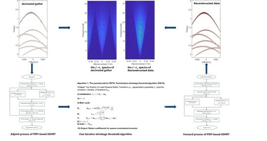
2.3. PSPI-Based Apex-Shifted Hyperbolic Radon Transform

Due to the mathematical similarity between the ASHRT operator’s description and the kinematic post-stack time migration equation, we introduce time-domain PSPI imaging and modeling operators to implement ASHRT. In this context, the imaging operator, which folds hyperbolic events to their vertices, is equivalent to the L T operator in the top-shifted hyperbolic Radon transform. Similarly, the modeling operator, which transforms the Radon domain model back to t x domain data, is equivalent to the L operator in the apex-shifted hyperbolic Radon transform. They are defined as follows:
L T = F F T k x 1 A I θ T F F T x , t  
L = F F T k x , ω 1 I θ A T F F T x  
where F F T k x 1 is the 1D Fourier inverse transform along, k x direction and F F T x is the 1D Fourier transform along the x direction; A is the summation operator and A T is the inverse operator of A ; θ and θ T are the extension operators for phase-shift modeling and imaging; I is the Lagrangian interpolation operator; F F T x , t is the 2D Fourier transform and F F T k x , ω 1 is the 2D Fourier inverse transform.
The flow of ASHRT implementation based on the PSPI operator is shown in Figure 1 and Figure 2.

2.4. Sparsity Promotion of Apex-Shifted Hyperbolic Radon Transform

In the process of solving Radon transform, for the solution of d = L m (the data in time-offset domain are solved according to Radon domain data), the obtained d is often ill-posed, and the obtained d does not satisfy the existence, uniqueness, and stability. To solve these problems, it is often necessary to determine a unique and stable solution with some prior information given in a fixed or random form. This method is known as regularization, and the corresponding approach to constructing the objective function is as follows:
Firstly, define an objective function:
J = d L m p p
The regularization process involves adding a regularization term to this objective function. For the equation d = L m , the objective function can be constructed:
J = d L m p p + λ m q q    
where J is the defined objective function. λ is a balancing parameter for the tradeoff between data mismatch and regularization terms. As λ increases, the Radon coefficients become sparser. However, when λ reaches a certain threshold, the regularization term becomes dominant, reducing the constraint on the error in the objective function. If λ is excessively large, the Radon coefficients may become overly sparse, leading to the loss of important information after transformation. Therefore, choosing an appropriate λ value is crucial to balance the sparsity of the model and the fidelity of data recovery. The variables p and q represent different norms used to measure vector sparsity. When different values of p and q are chosen, the solutions for Radon coefficients will also differ. A common approach is to use the l 2 norm ( p = 2 ) for the mismatch term and the l 1 norm ( q = 1 ) for data regularization.
To address this mixed l 1 l 2 optimization problem, various sparse constraint inversion algorithms are often introduced. The Fast Iterative Shrinkage-Thresholding Algorithm (FISTA) [31] is an improved iteration process for faster convergence, higher computational efficiency, and more accurate results. The iterative process is as follows:
To begin, initialize t 1 = 1 and Y 1 = m 0 , where m 0 is typically the Radon domain coefficients obtained directly from the original data’s Radon transform or the solution from the least-squares Radon transform.
m k + 1 = s o f t Y k + L T d L Y k α , λ 2 α  
t k + 1 = 1 + 1 + 4 t k 2 2
Y k + 1 = m k + 1 + t k 1 t k + 1 m k + 1 m k  
where k represents the current iteration number, soft is the soft-thresholding operator, λ is the regularization coefficient, and α is a control parameter known as the Lipschitz constant, where α m a x e i g L T L . By selecting the appropriate values for λ and α, you can ensure that the iteratively obtained solution maintains high fidelity and signal-to-noise ratio. The pseudocode for this algorithm (Algorithm 1) is as follows:
Algorithm 1: The pseudocode for FISTA: Fast iterative shrinkage threshold algorithm (FISTA)
1) Input: The Solution of Least Squares Radon Transform m 0 , regularization parameter λ , Lipschitz constant α , Number of iterations N i t e r
2) Initialization:  t 1 = 1 ,   Y 1 = m 0
3)  k 2
4) Main cycle:
5)        m k + 1 = s o f t Y k + L T d L Y k α , λ 2 α
6)            t k + 1 = 1 + 1 + 4 t k 2 2
7)       Y k + 1 = m k + 1 + t k 1 t k + 1 m k + 1 m k
8)  k k + 1
9) Until  k = N i t e r
10) Output: Radon coefficients for sparse constrained inversion

3. Results

3.1. Synthetic Example

We evaluated the proposed ASHRT algorithm using synthetic data. The synthetic data consists of four reflection events and two diffraction events. The reflection interfaces include two horizontal interfaces and two inclined interfaces. The final synthetic data is shown in Figure 3a, with a sampling interval of 0.008 s and receiver spacing of 10 m. The input to the interpolation algorithm is obtained by keeping one in every two traces of the initial data as shown in Figure 3b. Figure 3c,d show the f k x spectra corresponding to Figure 3a,b, respectively. We applied ASHRT based on the Stolt-stretch operator and the PSPI operator for interpolation of the decimated gather. The results are presented in Figure 4, where Figure 4a shows the interpolation result based on the Stolt-stretch operator, Figure 4c shows the corresponding interpolation error, Figure 4b shows the interpolation result based on the PSPI operator, and Figure 4d shows the corresponding interpolation error. In addition, Figure 4e–h are the f k x spectra corresponding to Figure 4a–d, respectively. It can be observed that the interpolation result based on the PSPI operator outperforms the interpolation result based on the Stolt-stretch operator. Additionally, we analyzed the amplitude spectra of the 50th and 190th traces of the data, as shown in Figure 5. The interpolation based on the PSPI operator has a better fit with the original data compared to the interpolation based on the Stolt-stretch operator. Figure 6 displays the objective function curves for both ASHRT methods. The PSPI operator exhibits better convergence compared to the Stolt-stretch operator.
We quantitatively analyzed the interpolation results of the two interpolation algorithms, and calculated the peak signal-to-noise ratio (PSNR), the signal-to-noise ratio (SNR), and the mean square error (MSE) of the two interpolation methods to evaluate the interpolation quality of this synthetic data, and the results are shown in Table 1:
Comparing the three indexes in Table 1, it can be seen that the interpolation results of the ASHRT interpolation method based on PSPI algorithm for synthetic data are better than those of ASHRT interpolation method based on Stolt-stretch algorithm.

3.2. Field Example

We also tested the interpolation algorithm on the marine data acquisition shown in Figure 7a. The data used an airgun source, which was carried on board along with the towline survey line used for data acquisition, and the geophone was a common piezoelectric geophone. The test data consisted of 200 channels of data with a data sampling interval of 8 ms and a receiver spacing of 12.5 m. The inputs to the interpolation algorithm are realized by retaining four traces out of every five initial data, as shown in Figure 7b. This ended up leaving 40 traces of data missing from the data. Figure 7c,d depicts the f k x spectra for Figure 7a,b, respectively. Figure 8 shows the decimated ways for the data of Figure 7b, with the corresponding decimated traces shown as red lines in the figure. We applied the ASHRT based on the Stolt-stretch operator and the ASHRT based on the PSPI operator for interpolation, and the results are presented in Figure 9. It is evident that the interpolation results using the PSPI operator outperform those using the Stolt-stretch operator. Figure 10 shows the convergence curves of the inversion process, indicating that the PSPI operator achieves better convergence compared to the Stolt-stretch operator.
Similarly, for the field data, we quantitatively analyzed the interpolation results of the two interpolation algorithms and calculated the peak signal-to-noise ratio, signal-to-noise ratio, and mean square deviation of the two interpolation methods to evaluate the interpolation quality of this field data, and the results are shown in Table 2.
Comparing the three indexes in Table 2, it can be seen that the interpolation results of the ASHRT interpolation method based on the PSPI operator are better than those of the ASHRT interpolation method based on the Stolt-stretch operator for the field data.

4. Conclusions

Pre-stack seismic data reconstruction is crucial in seismic data processing, and ASHRT is a highly effective reconstruction algorithm. Traditional ASHRT based on the Stolt-stretch operator has limitations in adapting to changes in medium velocity, resulting in some loss in the recovery of effective signals. This paper introduces a new ASHRT that considers the adaptability of the transformation operator to changes in medium velocity, aiming to better reconstruct seismic data.
The new ASHRT is implemented using the PSPI imaging and modeling operator. The advantage of the new operator is that it adapts to the case of transverse velocity variations in the medium, showing better results in the case of transverse variable velocity modeling and improving the signal-to-noise ratio of the reconstructed data. The results of related cases and actual data processing show that the proposed method is an effective interpolation technique. It recovers the attenuated data well and retains the effective signal. However, the method proposed in this paper also has certain limitations, which will have a greater impact when performing data reconstruction if the underground medium is more complex and the lateral velocity changes drastically.

Author Contributions

All authors made significant contributions to this paper. Y.W.: Algorithm writing, data analysis, and original manuscript writing. X.G.: Supervision, conceptualization, and manuscript editing. B.H.: Investigation, development of ideas, and reviewing the manuscript. All authors have read and agreed to the published version of the manuscript.

Funding

This research was supported by the National Natural Science Foundation of China (Subject No. 42074151). This project is supported by a special fund of Key Laboratory of Geophysical Exploration Equipment, Ministry of Education (Jilin University).

Data Availability Statement

The original contributions presented in the study are included in the article, further inquiries can be directed to the corresponding author.

Conflicts of Interest

The authors declare no conflicts of interest.

References

  1. Vermeer, G.J.O. Seismic Wavefield Sampling; Society of Exploration Geophysicists and Shell Research BV: Houston, TX, USA, 1990. [Google Scholar]
  2. Chen, Y.; Chen, K.; Shi, P.; Wang, Y. Irregular seismic data reconstruction using a percentile-half-thresholding algorithm. J. Geophys. Eng. 2014, 11, 065001. [Google Scholar] [CrossRef]
  3. Trad, D. Five-dimensional interpolation: Recovering from acquisition constraints. Geophysics 2009, 74, 123–132. [Google Scholar] [CrossRef]
  4. Duijndam, A.J.W.; Schonewille, M.A. Nonuniform fast Fourier transform. Geophysics 1999, 64, 539–551. [Google Scholar] [CrossRef]
  5. Ouyang, Z.; Zhang, L.; Wang, H.; Yang, K. High-Dimensional Seismic Data Reconstruction Based on Linear Radon Transform–Constrained Tensor CANDECOM/PARAFAC Decomposition. Remote Sens. 2022, 14, 6275. [Google Scholar] [CrossRef]
  6. Trad, D.; Ulrych, T.; Sacchi, M. Accurate interpolation with high resolution time-variant Radon transforms. Geophysics 2002, 67, 644–656. [Google Scholar] [CrossRef]
  7. Wang, J.; Ng, M.; Perz, M. Seismic data interpolation by greedy local Radon transform. Geophysics 2010, 75, WB225–WB234. [Google Scholar] [CrossRef]
  8. Hollander, Y.; Yilmaz, O. An acceleration method for the anti-leakage parabolic Radon transform for seismic data interpolation. In Proceedings of the SEG International Exposition and Annual Meeting, San Antonio, TX, USA, 15–20 September 2019; SEG: Houston, TX, USA, 2019; p. D033S045R005. [Google Scholar] [CrossRef]
  9. Naghizadeh, M.; Sacchi, M. Beyond alias hierarchical scale curvelet interpolation of regularly and irregularly sampled seismic data. Geophysics 2010, 75, 189–202. [Google Scholar] [CrossRef]
  10. Kong, L.Y.; Yu, S.W.; Chen, L. Application of compressive sensing to seismic data reconstruction. Acta Seismol. Sin. 2012, 34, 659–666. [Google Scholar]
  11. Gan, S.; Wang, S.; Chen, Y.; Zhang, Y.; Jin, Z. Dealiased seismic data interpolation using seislet transform with low-frequency constraint. IEEE Geosci. Remote Sens. Lett. 2015, 12, 2150–2154. [Google Scholar]
  12. Fomel, S. Towards the seislet transform. In Proceedings of the 2006 SEG Annual Meeting, New Orleans, LO, USA, 1–6 October 2006; pp. 2847–2851. [Google Scholar]
  13. Liu, Y.; Fomel, S. OC-seislet: Seislet transform construction with differential offset continuation. Geophysics 2010, 75, 235–245. [Google Scholar] [CrossRef]
  14. Gong, X.; Wang, S.; Zhang, T. Velocity analysis using high-resolution semblance based on sparse hyperbolic Radon transform. J. Appl. Geophys. 2016, 134, 146–152. [Google Scholar] [CrossRef]
  15. Dix, C.H. Seismic velocities from surface measurements. Geophysics 1955, 20, 68–86. [Google Scholar] [CrossRef]
  16. Trad, D. Interpolation and multiple attenuation with migration operators. Geophysics 2003, 68, 2043–2054. [Google Scholar] [CrossRef]
  17. Trad, D.; Siliqi, R.; Poole, G.; Boelle, J. Fast and robust deblending using Apex shifted Radon transform. In SEG Technical Program Expanded Abstracts; Society of Exploration Geophysicists: Houston, TX, USA, 2012; pp. 1–5. [Google Scholar] [CrossRef]
  18. Sabbione, J.I.; Sacchi, M.D.; Velis, D.R. Microseismic data denoising via an apex-shifted hyperbolic Radon transform. In Proceedings of the 83rd Annual International Meeting, SEG, Expanded Abstracts, Houston, TX, USA, 22–27 September 2013; pp. 2155–2161. [Google Scholar] [CrossRef]
  19. Karimpouli, S.; Malehmir, A.; Hassani, H.; Khoshdel, H.; Nabi-Bidhendi, M. Automated diffraction delineation using an apex-shifted Radon transform. J. Geophys. Eng. 2015, 12, 199–209. [Google Scholar] [CrossRef]
  20. Li, C.; Peng, S.; Zhao, J.; Cui, X.; Du, W.; Satibekova, S. Polarity-preserved diffraction extracting method using modified apex-shifted Radon transform and double-branch Radon transform. J. Geophys. Eng. 2018, 15, 1991–2000. [Google Scholar] [CrossRef]
  21. Seher, T. A high-resolution apex-shifted hyperbolic Radon transform and its application to multiple attenuation. In Proceedings of the SEG International Exposition and Annual Meeting, Houston, TX, USA, 24–29 September 2017; SEG: Houston, TX, USA, 2017; p. SEG-2017-17640537. [Google Scholar]
  22. Yang, F.; Wang, D.; Hu, B.; Zhu, H.; Sun, J. 3D surface-related multiples elimination based on improved apex-shifted Radon transform. Acta Geophys. 2021, 69, 1679–1696. [Google Scholar] [CrossRef]
  23. Ibrahim, A.; Sacchi, M.D. Fast simultaneous seismic source separation using Stolt migration and demigration operators. Geophysics 2015, 80, WD27–WD36. [Google Scholar] [CrossRef]
  24. Ibrahim, A.; Terenghi, P.; Sacchi, M.D. Wavefield reconstruction using a Stolt-based asymptote and apex shifted hyperbolic Radon transform. In Proceedings of the 2015 SEG Annual Meeting, New Orleans, LO, USA, 18–23 October 2015. SEG Technical Program Expanded Abstracts. [Google Scholar] [CrossRef]
  25. Gong, X.; Wang, S.; Du, L. Seismic data reconstruction using a sparsity-promoting apex shifted hyperbolic radon-curvelet transform. Stud. Geophys. Geod. 2018, 62, 450–465. [Google Scholar] [CrossRef]
  26. Gong, X.; Yu, C.; Wang, Z. Separation of prestack seismic diffractions using an improved sparse apex-shifted hyperbolic Radon transform. Explor. Geophys. 2017, 48, 476–484. [Google Scholar] [CrossRef]
  27. Yilmaz, O.G. Seismic Data Analysis: Processing, Inversion, and Interpretation of Seismic Data, 2nd ed.; Investigations in Geophysics; SEG: Houston, TX, USA, 2001. [Google Scholar]
  28. Gazdag, J.; Sguazzero, P. Migration of seismic data by phase shift plus interpolation. Geophysics 1984, 49, 124–131. [Google Scholar] [CrossRef]
  29. Gazdag, J. Wave equation migration with the phase-shift method. Geophysics 1978, 43, 1342–1351. [Google Scholar] [CrossRef]
  30. Claerbout, J. Earth Soundings Analysis: Processing Versus Inversion; Blackwell Scientific Publications: Hoboken, NJ, USA, 1992. [Google Scholar]
  31. Beck, A.; Teboulle, M. Fast gradient-based algorithms for constrained total variation image denoising and deblurring problems. IEEE Trans. Image Process. 2009, 18, 2419–2434. [Google Scholar] [CrossRef] [PubMed]
Figure 1. Adjoint process of PSPI-based ASHRT.
Remotesensing 16 01114 g001
Figure 2. Forward process of PSPI-based ASHRT.
Remotesensing 16 01114 g002
Figure 3. Simple synthetic data example: (a) original gather. (b) decimated gather, and (c,d) are the f k x spectra of (a,b), respectively.
Remotesensing 16 01114 g003
Figure 4. Interpolation results for simple synthetic data: (a) ASHRT interpolation based on the Stolt-stretch operator, (b) ASHRT interpolation based on the PSPI operator, (c) Interpolation error for ASHRT based on the Stolt-stretch operator, (d) Interpolation error for ASHRT based on the PSPI operator, and (eh) are the f k x spectra of (ad), respectively.
Remotesensing 16 01114 g004
Figure 5. Amplitude spectra interpolation results for the simple synthetic data: (a) Amplitude spectrum for the 50th trace of the original data (black curve), amplitude spectrum interpolated by Stolt-stretch-based ASHRT (red curve), amplitude spectrum interpolated by PSPI-based ASHRT (blue curve). (b) Amplitude spectrum for the 190th trace of the original data (black curve), amplitude spectrum interpolated by Stolt-stretch-based ASHRT (red curve), amplitude spectrum interpolated by PSPI-based ASHRT (blue curve).
Remotesensing 16 01114 g005
Figure 6. Objective function curves for simple synthetic data.
Remotesensing 16 01114 g006
Figure 7. Filed data example: (a) Original gather, (b) decimated gather, and (c,d) are the f k x spectra of (a,b), respectively.
Remotesensing 16 01114 g007
Figure 8. Decimated ways of the data in Figure 7b: The red part represents the decimated trace.
Remotesensing 16 01114 g008
Figure 9. Interpolation results for filed data: (a) ASHRT interpolation based on the Stolt-stretch operator, (b) ASHRT interpolation based on the PSPI operator, (c) Interpolation error for ASHRT based on the Stolt-stretch operator, (d) Interpolation error for ASHRT based on the PSPI operator, and (eh) are the f k x spectra of (ad), respectively.
Remotesensing 16 01114 g009
Figure 10. Objective function curves for filed data.
Remotesensing 16 01114 g010
Table 1. Simple model example.
PSNR/dbSNR/dbMES
Stolt-stretch-based ASHRT48.7013.791.35 × 10−5
PSPI-based ASHRT53.2722.904.71 × 10−6
Table 2. Filed data example.
PSNR/dbSNR/dbMES
Stolt-stretch-based ASHRT20.666.560.0086
PSPI-based ASHRT22.138.000.0061
Disclaimer/Publisher’s Note: The statements, opinions and data contained in all publications are solely those of the individual author(s) and contributor(s) and not of MDPI and/or the editor(s). MDPI and/or the editor(s) disclaim responsibility for any injury to people or property resulting from any ideas, methods, instructions or products referred to in the content.

