Article

Spatial Quantification of Cropland Soil Erosion Dynamics in the Yunnan Plateau Based on Sampling Survey and Multi-Source LUCC Data

1
Faculty of Land Resource Engineering, Kunming University of Science and Technology, Kunming 650093, China
2
Key Laboratory of Plateau Remote Sensing, Yunnan Provincial Department of Education, Kunming 650093, China
3
Institute of International Rivers and Eco-Security, Yunnan University, Kunming 650091, China
4
Yunnan Key Laboratory of Soil Erosion Prevention and Green Development, Yunnan University, Kunming 650091, China
5
Yuanjiang Dry-Hot Valley Water and Soil Conservation Observation and Research Station of Yunnan Province, Yunnan University, Kunming 650091, China
6
Institute of Geographic Sciences and Natural Resources Research, Chinese Academy of Sciences, Beijing 100101, China
7
Aerospace Information Research Institute, Chinese Academy of Sciences, Beijing 100101, China
8
International Research Center of Big Data for Sustainable Development Goals, Beijing 100094, China
9
National Engineering Research Center for Geomatics (NCG), Chinese Academy of Sciences, Beijing 100101, China
10
State Key Laboratory of Simulation and Regulation of Water Cycle in River Basins, China Institute of Water Resources and Hydropower Research, Beijing 100048, China
11
Research Center of Soil and Water Conservation of the Ministry of Water Resources, Beijing 100048, China
*
Author to whom correspondence should be addressed.
Remote Sens. 2024, 16(6), 977; https://doi.org/10.3390/rs16060977
Submission received: 14 January 2024 / Revised: 6 March 2024 / Accepted: 8 March 2024 / Published: 10 March 2024
(This article belongs to the Special Issue Soil Erosion Estimation Based on Remote Sensing Data)

Abstract

:
The mapping and dynamic monitoring of large-scale cropland erosion rates are critical for agricultural planning but extremely challenging. In this study, using field investigation data collected from 20,155 land parcels in 2817 sample units in the National Soil Erosion Survey, as well as land use change data for two decades from the National Land Use/Cover Database of China (NLUD-C), we proposed a new point-to-surface approach to quantitatively assess long-term cropland erosion based on the CSLE model and non-homologous data voting. The results show that cropland in Yunnan suffers from serious problems, with an unsustainable mean soil erosion rate of 40.47 t/(ha·a) and an erosion ratio of 70.11%, which are significantly higher than those of other land types. Engineering control measures (ECMS) have a profound impact on reducing soil erosion; the soil erosion rates of cropland with and without ECMs differ more than five-fold. Over the past two decades, the cropland area in Yunnan has continued to decrease, with a net reduction of 7461.83 km2 and a ratio of −10.55%, causing a corresponding 0.32 × 10⁸ t (12.12%) reduction in cropland soil loss. We also quantified the impact of different LUCC scenarios on cropland erosion, and extraordinarily high variability was found in soil loss in different basins and periods. Conversion from cropland to forest contributes the most to cropland erosion reduction, while conversion from grassland to cropland contributes 56.18% of the increase in soil erosion. Considering the current speed of cropland regulation, it is the sharp reduction in land area that leads to cropland erosion reduction rather than treatments. The choice between the Grain for Green Policy and Cropland Protecting Strategy in mountainous areas should be made carefully, with understanding and collaboration between different roles.

1. Introduction

Soil, one of Earth’s most precious and threatened resources [1], provides humans with far more than food, but also a large variety of services such as biomass production, water filtration, nutrient transformation, carbon storage and habitat and terrestrial biodiversity maintenance [2,3]. However, most soil resources worldwide are in poor health, and accelerated soil erosion induced by inappropriate human activities and related land use changes are the primary drivers behind the problem [4,5]. Soil erosion refers to the complex process of soil material detachment, transportation, and deposition by external erosive forces. It has the on-farm impacts of reduced soil fertility and productivity [6,7], and also leads to greater off-site costs such as those related to muddy flooding, sedimentation and water pollution [8,9], threatening global biogeochemical cycles [10,11]. Theoretical and runoff plot observations have demonstrated that cropland is the main source of soil loss [5,12,13], where the soil erosion rates can be orders of magnitude greater than the speed of natural soil formation as well as the rates on other land use types [13,14], especially in mountainous areas. It is estimated that about 80% of the agricultural land around the world is suffering from serious erosion problems, with an unsustainable mean annual cropland erosion rate of about 30 t/(ha·a). Consequently, more than one-third of cropland has vanished in the last few decades due to soil erosion [15,16]. To monitor and assess the impacts of soil erosion and develop strategies to deal with them, the mapping of up-to-date quantitative information on cropland erosion rates at the regional scale is essential, but also very challenging [17,18], since for most areas worldwide the observed erosion data are woefully inadequate.
On the one hand, it is difficult to gain insights into the spatial patterns of soil erosion without information on specific soil erosion rates and hotspots; confusion arises in the allocation of soil erosion mitigation programs and priorities, the formulation of policies and evaluations of the effectiveness of soil conservation measures [19]. Besides this, knowledge gaps are generated in critical fields like climate change, landslide and flood prediction, carbon mitigation scenarios and earth science modeling, and the well-known polices of SDGs, CAP, UNCCD and IPBES have not been addressed [20]. Despite this, soil erosion modeling and prediction have received considerable attention from governments and scientists for more than seven decades [21,22], with various empirical, conceptual and physically based models and approaches developed to measure, estimate and monitor soil erosion from the field to the landscape scale [23,24,25,26]. Yet, most models are only applicable to micro-scales, such as field plots, hillslopes and small catchments, and are difficult to apply to large scales due to the spatial heterogeneity of the factors affecting soil erosion [27,28], as well as scale issues [29], model limitations and applicability [27,29,30], and the high demands of models for input data [20,31]. Most empirical soil erosion models are based on the scales of plots and hillslopes, with specific applicable conditions and scopes [29]. For example, the most widely applied soil erosion prediction models, of the USLE type, were originally developed at the plot scale for agricultural lands (gradients less than 18%), based on the “unit plot concept” of a 22.1 m long and 1.83 m wide plot, with a 9% slope and up- and downhill tillage [20]. The major limitation of soil erosion modeling for any given area is that the microscopic processes involved are less closely considered, and it is difficult to acquire up-to-date soil erosion information such as that regarding crop rotation, terracing, mulching, contouring and hedgerow planting at large scales, especially in fragmented mountainous landscapes. When upscaling the models to large scales, the input variables or parameters of the models are simplified for the sake of generalization, and huge uncertainties may thus lead to extrapolation errors, meaning the reliability of the results is often questioned [20,29]. Currently, the contradiction between the relatively low resolution of available input data and the high resolution required for runoff–erosion processes is a major obstacle to overcome in the context of the large-scale dynamic quantification of soil erosion [29]. For mountainous areas, poor data availability, timeliness and data quality have been the biggest obstacles when mapping and visualizing soil erosion rates at large scales [31].
To date, limited by the over-parameterization of physical models and the poor quality of the datasets available, large-scale soil erosion assessment methods are generally based on empirical models, and can be divided into the two categories of sampling surveys and remote sensing assessments [19,32,33]. (a) Sampling survey is a method of allocating samples within a region according to certain proportions and rules. Field investigations on erosion features and parameters are then conducted, after which soil erosion models can be further applied to quantify soil erosion rates or conditions, and statistical methods can then be used to estimate the overall soil erosion patterns of the region. The typical examples are the National Resource Inventory (NRI), conducted in the United States [34], the National Soil Erosion Survey in China [35], the EUSEDcollab network [36] and gully erosion monitoring based on the Land Use/Cover Area frame survey in Europe [36]. (b) Another category is remote sensing-based assessments using simplified models. Since the large-scale application of complex models is challenging, as the availability of high-resolution remote sensing images increases, large-scale estimation using empirical models such as USLE/RUSLE is becoming feasible due to the relatively simple nature of the input data [20]. Compared with field investigations, satellite remote sensing is characterized by the acquisition of timely, affordable data that are uniform over large areas, the capacity for real-time information acquisition and the use of a regular revisit wide-view field, and it has been widely applied in soil erosion modeling and mapping [37,38]. In particular, efforts have been made towards direct soil erosion detection [37,39], as well as the estimation of parameters of rainfall erosivity [40,41], soil-related property derivation [42], topographic factors extraction [43], cover management (C-factor) and support practices (P-factor) [44,45,46,47], the mapping of specific soil conservation measures using high-resolution images [48,49,50] and large-scale soil erosion assessments with raster layer operations [51,52]. The biggest advantage of the sampling survey approach is that it provides reliable soil erosion rates, and large-scale spatial patterns of soil erosion status can be derived by combination with statistical principles [53,54,55], but the field measurement and investigation of indices are labor-intensive and costly processes. Remote sensing-based methods allow for rapid and efficient soil erosion assessment even in areas where intensive field investigation is a challenge, but in a more qualitative or semi-quantitative way. Although high-resolution imagery like SPOT 5, IKONOS and QuickBird impart high-quality data in erosion mapping, their utility remains hindered as large-area imagery is also unattainable for most countries [37].
Previous studies [56,57,58,59] have confirmed that land use/cover change (LUCC) is the primary cause of accelerated soil erosion under climate change scenarios, and is the most direct and informative reflection of the interaction between human activities and the soils on the Earth’s surface [60]. For most cases, the key to prevent soil erosion is to change various unreasonable land uses to a sustainable mode in line with the principles of sustainable development, such as returning farmland to forest/grassland and converting slopes into terraces in China. Meanwhile, compared with the inversion of soil erosion indices, the use of remote sensing in LUCC monitoring is the field with the most complete and mature technology. At large scales, by integrating the most commonly used Landsat series data imagery, relevant studies [61,62] have also revealed the long-term impacts of land use changes on soil erosion, and provide the information necessary for assessing soil erosion intensity. However, due to the lack of field-based soil erosion data, the dynamic results of estimation generally regard potential soil erosion risks without exact dynamic soil erosion rates. Obviously, more detailed field experiment-derived data that accurately quantify soil erosion rates are needed.
In 2010 through 2012, the Ministry of Water Resources of China (MWRC) conducted the first ever field-based National Soil Erosion Survey (NSES) in history, using a sampling survey and the Chinese Soil Loss Equation (CSLE) [33,63,64]. These detailed onsite investigations have provided abundant information on soil erosion rates at the land parcel scale, thus reducing the uncertainties in soil erosion modeling and prediction [65]. Soil erosion is a dynamic process that demands constant monitoring in order to derive up-to-date information on its spatial pattern [37]. The combination of the advantages that can be derived from a combination of sampling surveys and remote sensing is the most feasible solution to large-scale soil erosion rate quantification. The objective of this paper is thus to quantitatively assess the cropland soil erosion dynamics induced by long-term cropland changes in mountainous areas, approached from the perspectives of soil erosion field investigations and LUCC scenarios based on time series satellite images.

2. Materials and Methods

2.1. Study Area

Yunnan Plateau (20°8′–29°16′N, 97°31′–106°12′E) is a low-latitude highland region situated in the southwest border region of China. It covers a total area of about 3.83 × 10⁵ km2, and borders the Himalayan Range, Myanmar, Laos and Vietnam (Figure 1). Mostly mountainous in character, 94% of the province is dominated by mountains and plateaus, only 6% of which comprises small interspersed scattered valley basins. The landscape tilts downward from the northwest to the southeast, and the elevation ranges from 76 m to 6740 m above sea level, with an average altitude of 2000 m [65].
Affected by the Indian and East Asian monsoons and air masses from the Qinghai–Tibet Plateau, the region has a subtropical plateau monsoon climate with substantial variations, though it is relatively mild due to the elevation. The mean annual precipitation varies from 600 in dry–hot valleys to 2300 mm in the southern and western mountains, with over half of the rain occurring between June and August, while the dry season (November to April of the following year) accounts for only 20% or less of the 1100 mm annual precipitation. The annual average temperatures in the winter and summer are 6–8 °C and 19–22 °C, respectively [66,67]. Soils in Yunnan are generally rich in clay and formed under conditions of high precipitation and temperature, and include Acrisols, Cambisols and Luvisols. It is particularly worth mentioning that Yunnan has long been recognized as a hotspot for biodiversity in China. Taking vegetation resources as an example, tropical, seasonal, subtropical evergreen broad-leaved, temperate coniferous forests and meadow steppes can all be found in the region [68]. The landscape is dissected by the six major rivers of the Irrawaddy, Nu (Salween), Lancang (upper reach of the Mekong), Jinsha (upper reach of the Yangtze), Honghe and Pearl. The province also features the largest sloping cropland area in China, as the limited basin areas have already been fully utilized, meaning that the soil erosion pressure on the remaining land resources is extremely high.

2.2. Data Sources

2.2.1. Sampling Survey and Primary Sample Units (PSUs)

The sampling survey in the NSES was conducted using a non-equal probability sampling method (Figure 2a). In view of the dominant erosive force of soil loss and the integrity of county boundaries, the whole country was firstly divided into a water erosion region, a wind erosion region, a freeze–thaw erosion region and regions showing the co-occurrence of erosion types (Figure 2b).
Generally, uniform national gridding was employed for water erosion, which has the greatest implications. Four layers of grids were set with different grid sizes, including the county level (40 km × 40 km), the township level (10 km × 10 km), the control area level (5 km × 5 km) and the Primary Sample Units (1 km × 1 km). The grids were divided according to the Gauss–Krüger Projection zoning method, which divides the country into 3°-interval geographical zones (a total of 22 zones). In each zone, in the Y-axis direction, grids were divided on both sides based on the central meridian, and in the X-axis direction, grids were divided on both sides based on the equator. PSUs for water erosion were allocated, with four sampling densities of 4%, 1%, 0.25% and 0.0625% [32,33]. For the plain area, the PSU was a single 1 km × 1 km grid, while for the mountainous area, the PSU was a small watershed of 0.2–3.0 km2. The PSU here was a small geographical area with a fixed location and area that could express the basic characteristics of soil erosion and show spatial heterogeneity in soil erosion factors (especially soil conservation measures). For areas with glaciers, permanent snowfields, deserts, swamps, large lakes and reservoirs where no water erosion occurs, at high altitudes exceeding 4800 m (thus with lower human activities), water erosion was generally less notable [33,69]. Based on the erosion characteristics, human disturbance and accessibility of each province, a total of 33,966 PSUs were determined nationwide in the NSES (Figure 2d). Different from the NRI, in China, the NSES is actually an area-sampling survey rather than a point-sampling survey [63].
PSUs were the main focus of the field investigation and data collection in the NSES. Each PSU was then divided into pieces of land defined as a land parcel that share the same land types and conservation measures. The data gatherers were then trained to investigate each land parcel and collect information concerning the soil erosion factors of the CSLE, with uniform standards. Specifically, by using high-precision topographic maps as field survey base maps, detailed information regarding land parcel number, fraction vegetation coverage, canopy density, land use, vegetation type, engineering measures and crop rotation patterns was acquired. As it suffers from a serious water erosion problem, Yunnan drew a lot of attention in the NSES, and the numbers of both PSUs and land parcels selected were the largest among all provinces in China, at 2817 and 20,155, respectively (Figure 2c). All these field-derived data were provided by Beijing Normal University (the technical support unit of the NSES) [32,69].
In addition to the data derived from field investigations, critical data involved in calculating the annual average soil erosion rates were obtained nationwide as follows: (a) daily erosive rainfall (greater than 12 mm) data for three decades; (b) digital DEMs of 1:10,000 scale for each PSU to extract slope gradient and length; (c) more than 10,000 records of soil profile data and soil types at 1:500,000 scale retrieved from the Second National Soil Survey, and observed unit plot and cropland plot data; (d) time series multi-spectral reflectance data of Sentinel-2, Landsat TM/ETM/OLI images prepared to revise vegetation indices from 2000 to 2020; and (e) high-resolution satellite imagery for Yunnan, comprising GF-1 (2 m), GF-2 (1 m) and GF-7 (0.8 m) images and Beijing-2 (resolution of 0.65 m) at different periods, to optimize the land use map.
After standardizing the data processing, with each PSU containing 7 raster layers (spatial resolution of 10 m) of soil erosion factors in the CSLE model, the soil erosion modulus was then computed using the raster multiplication operation and statistical methods, and soil loss for each land use type was finally evaluated at the land parcel, PSU, province and national levels. Figure 3 presents the official procedure [32,33] for calculating soil erosion modulus in PSUs using the CSLE model and detailed information on a random PSU of a small watershed, and each land parcel within it. For this study, the most critical data concerned the multi-year average soil erosion rates of various land use parcels obtained based on field surveys, which were taken as the basis for comprehensive analyses of soil erosion distribution, area, ratio and intensity.

2.2.2. Land Use/Cover Change (LUCC) Dynamics

Initialized in the latter half of the 1990s, the National Land Use/Cover Database of China (NLUD-C) [70] has been applied to land use/cover-related research as the most well-known LUCC database in China for decades. By drawing boundaries and labeling attributes for each LUCC polygon based on Landsat TM/ETM/OLI images (resolution of 30 m), we have updated the database for several periods using the interactive interpretation method. The NLUD-C includes datasets of land use status and LUCC dynamics of China with a 5-year interval, and land use types are here classified into 6 first-level categories and 25 corresponding second-level classes.
Compared to the numerous LUCC products retrieved using automatic classification and change detection methods, the biggest advantage of NLUD-C lies in its use of professional knowledge, its uniformly interpretable symbols and its unified image acquisition phases before and after, which ensure the high accuracy of its information on land attributes. Although the OA of the NLUD-C is significantly higher than those of other similar products, distortion and inaccurate patch boundaries still occur in mountainous areas, since manual geometric correction is performed in different periods. At present, remote sensing LUCC data with a higher resolution may be a better choice for soil erosion modeling, as they reduce model uncertainty, but are also characterized by the shortcomings of high image acquisition costs and short time series. To optimize the accuracy of land use data, we employed NLUD-C as the main basis of the LUCC, supplemented by 7 publicly accessible non-homogeneous LUCC datasets, comprising the three long-term 30 m resolution products of GLC_FCS30 [71], CLCD [72] and GlobeLand30 [73], as well as the four short-term 10 m resolution products of ESRI_LandCover [74], ESA_WorldCover [75], CRLC [76] and Dynamic World from Google [77]. Detailed information on these land use datasets is listed in Table 1. In this study, land use maps of Yunnan in 2000, 2005, 2010, 2015 and 2020 have been prepared for further analysis.

2.3. Methods

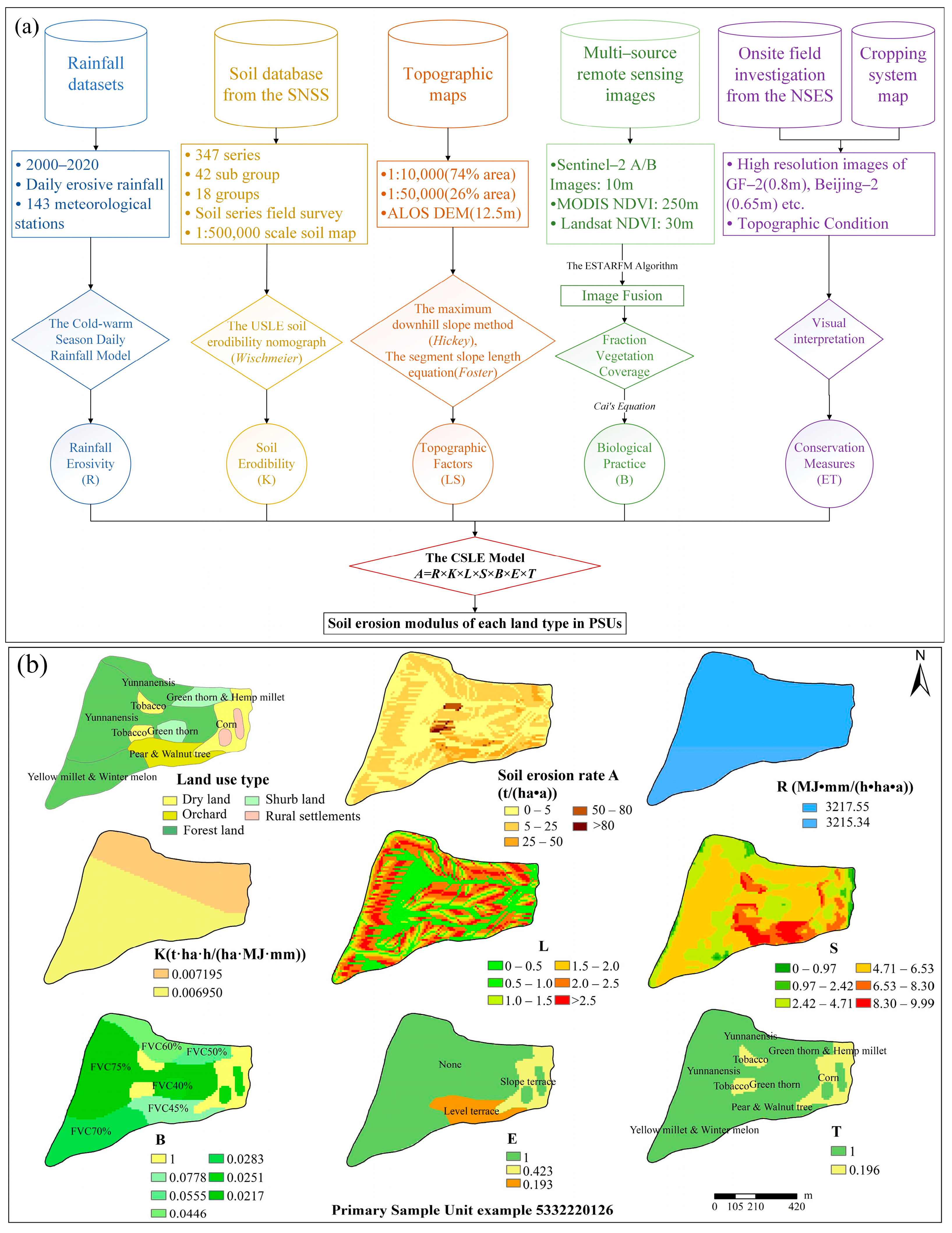
2.3.1. The CSLE Model

By adapting the parameters of the Universal Soil Loss Equation (USLE) to China, Liu et al. [33] developed a CSLE model based on data measured on Chinese unit plots and numerous plots modified to a unit plot. As the official model of the Ministry of Water Resources of China (MWRC) for soil erosion assessment, the differences between the CSLE and USLE regard modifications that elucidate crop systems, management, practices, soil types, rainfall patterns and topography in China.
CSLE is a model used to estimate annual soil loss by sheet and rill water erosion for a given combination of factors affecting soil erosion. The major advantage of CSLE is that it more closely reflects the topographical conditions and the actual situation of soil conservation measures in China, while the two factors of cover management and support practices (C, P) set out in the USLE have been modified into three factors of biological measures (B), engineering measures (E) and tillage measures (T) [64,78,79]. The five dimensionless factors of slope length, slope gradient, biological measure, engineering measure and tillage measure are used to modify the soil loss determined by the dimensional rainfall erosivity factor and soil erodibility factor in this model.
The principal equation of CSLE can be expressed as follows:
A = R × K × L × S × B × E × T
where A is the mean annual soil loss, with a unit of t/(hm2·a); R is the rainfall and runoff factor or rainfall erosivity, MJ·mm/(hm2·h·a); K is the soil erodibility factor, t·hm2·h/(MJ·hm2·mm); L is the slope length factor and S is the slope steepness factor; B is the biological measure factor; E is the engineering measure factor; and T is the factor of tillage measures. The B, E and T factors have a unitless range of 0–1, and the smaller the value is, the better the soil conservation effect of the related measure.
The specific methods of calculation for factors R, K, L and S are described in detail in our previous work [65,80,81] and in the related literature [69,82,83]. They can be listed as follows:
R = k = 1 24 R k
R k = 1 N i = 1 N j = 0 m ( α P i , j , k 1.7265 )
W R k = R k R
where k represents the 12 months in a year, Rk is the average rainfall erosivity in the k-th month (MJ∙mm∙ha−1∙h−1∙a−1), N refers to the time series, α takes a value of 0.3937 for the warm season and 0.3101 for the cold season, Pi,j,k is the actual erosive rainfall (≥12 mm) on the j-th day in the k-th month in the i-th year and m is the number of days with erosive rainfall in the corresponding month. WRk is the ratio of average rainfall erosivity in the k-th month to the average annual rainfall erosivity, which reflects the seasonal distribution of rainfall erosivity.
K = 2.1 × 10 4 M 1.14 ( 12 O M ) + 3.25 ( S 2 ) + 2.5 ( P 3 ) / 100
M = N 1 ( 100 N 2 )
M = N 1 ( N 3 + N 4 )
where N1 (particle size: 0.002–0.1 mm) is the percentage of silt (0.002–0.05 mm) plus very fine sand (0.05–0.1 mm), N2 (<0.002 mm) is the clay fraction, (100–N2) (0.002–2 mm) represents all soil fractions other than clay, OM is the soil organic matter content (%), S is the soil structure code and P is the soil permeability code.
S = 10.8   s i n   θ + 0.03 θ 5 ° 16.8   s i n   θ 0.50 5 ° < θ 10 ° 21.9   s i n   θ 0.96 θ > 10 °
L i = ( λ o u t m + 1 λ i n m 1 ) [ ( λ o u t λ i n ) × 22.13 m ] m = 0.2 θ 1 ° m = 0.3 1 ° < θ 3 ° m = 0.4 3 ° < θ 5 ° m = 0.5 θ > 5 °
where Li is the slope length factor of the i-th pixel, λout and λin are the pixel exit and entrance slope lengths and m is the slope length exponent depending on the slope.
F V C = N D V I m a x N D V I s o i l N D V I v e g N D V I s o i l
B = i = 1 12 B i R i i = 1 12 R i
B i = 1 F V C = 0 0.6508 0.3436 lg F V C × 100 0 < F V C 0.783 0 F V C > 0.783
where NDVImax refers to the regional maximum NDVI; NDVIveg is the NDVI value of the pure vegetation pixels; NDVIsoil is the NDVI value of the pure bare soil pixels; Bi is the B-factor of the i-th month. The relationship between the FVC and B values can be determined using Equation (12). The ET factors in the CSLE are mainly collected from field surveys, with reference to the corresponding values derived from runoff plot experiments performed by local experts and an extensive literature review on the national level.

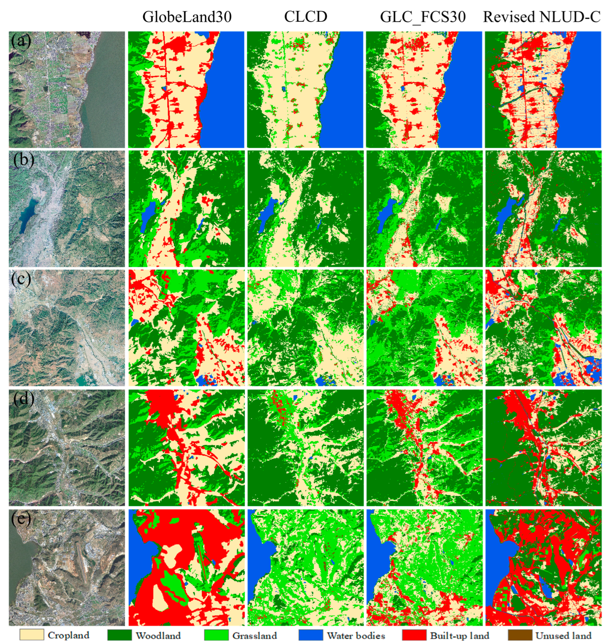
2.3.2. Non-Homogeneous Data Voting and LUCC Optimization

The rapid development of remote sensing technology provides a key technical approach to obtain comprehensive information on large-scale land use/cover distribution and changes. In recent years, scientists worldwide have incorporated image processing methods to interpret and analyze remote sensing images, and produced numerous LUCC products with different spatial resolutions.
Our evaluation of the accuracy of datasets and extensive literature review demonstrate that automatic image classification and change detection approaches can provide satisfactory results only when applied to certain land use types with homogeneous colors and textures, such as water bodies, built-up land and bare rock [70]. Due to the differences between satellite sensors, processing methods and classification systems, the capacities of different LUCC products to describe Earth surface conditions are also different, especially in fragmented mountainous areas like Yunnan, affected by cloudy and rainy weather, where high-quality image availability is hard to come by, making the difference even more significant. As a result, the reliability of data is often questioned. For example, despite the 8 datasets we mentioned above sharing similar definitions of cropland, the cropland areas of Yunnan in 2020 provided by them are totally different. The cropland areas of the 4 long time series 30 m datasets were 6.74 × 10⁴ km2 for NLUD-C, 3.24 × 10⁴ km2 for GLC_FCS30, 8.39 × 10⁴ km2 for CLCD and 10.99 × 10⁴ km2 for GlobeLand30, while the cropland areas of the 4 recent 10 m datasets were 3.58 × 10⁴ km2 for ESRI_LC, 5.09 × 10⁴ km2 for ESA_WC, 9.77 × 10⁴ km2 for CRLC and 2.50 × 10⁴ km2 for Dynamic World, respectively. For Yunnan, based on our field surveys, CLCD significantly underestimates the impervious area, GLC_FCS30 generally underestimates the cropland area, GlobeLand30 significantly overestimates the cropland area, ESRI_LC and Dynamic World significantly overestimate the impervious area, CRLC misclassifies woodland into cropland and ESA_WC misclassifies impervious area into bare land. Misclassification, omissions and high degrees of confusion between grassland and shrub can be found in almost all of the datasets. High-resolution datasets do not always provide more reliable information, and significant differences can be found at the same resolution. Obviously, the overall accuracy of global or national-scale LUCC datasets in local areas needs to be verified, since the verification methods and reference data used by the datasets are different, meaning that the independent accuracy assessments cannot be directly compared [84]. Therefore, a critical evaluation of the suitability and optimization of LULC products based on application purposes should be performed before use.
For plateau mountain areas like Yunnan, long-term high-resolution (higher than 10 m) LUCC data have been inaccessible and impractical so far. Here, we employ the non-homologous data voting method [85] to modify and optimize the NLUD-C data. The concept of non-homogeneous data voting originates from pure pixels in image classification. The basic idea is to determine the consistency of the classification results of the same feature by multiple datasets through spatial overlay analysis on the basis of a standardized and unified classification system. For pixels with high consistency, the original classification results will continue to be used, and for pixels with low consistency, reclassification and optimization will then be processed. Non-homogeneous data voting can, to some extent, effectively solve the problem of the broad representativeness and authenticity of sample data. Specifically, we select geometrically fine time series-corrected Landsat images from October to February in each year to ensure the uniformity of multiple phases. Based on NLUD-C, with clear interpretation symbols and professional knowledge, non-homologous data voting was then performed to analyze the classification consistency. For areas with a high degree of consistency, we kept the first-level type to reduce uncertainty, while for areas with a high degree of confusion, especially for basin valleys and urban peripheral areas with frequent human activities and dramatic changes, high-resolution remote sensing images were used to assist in the precise visual interpretation. Finally, the time series LUCC data obtained combined the advantages of multiple datasets and avoided the respective shortcomings. Figure 4 presents the workflow of the non-homologous data voting method used for modifying the LUCC data, and Figure 5 shows our revised NLUD-C results for a typical inter-mountain basin. Using high-resolution remote sensing images, we also compared them to three other time series land use products for different underlying surfaces.

3. Results

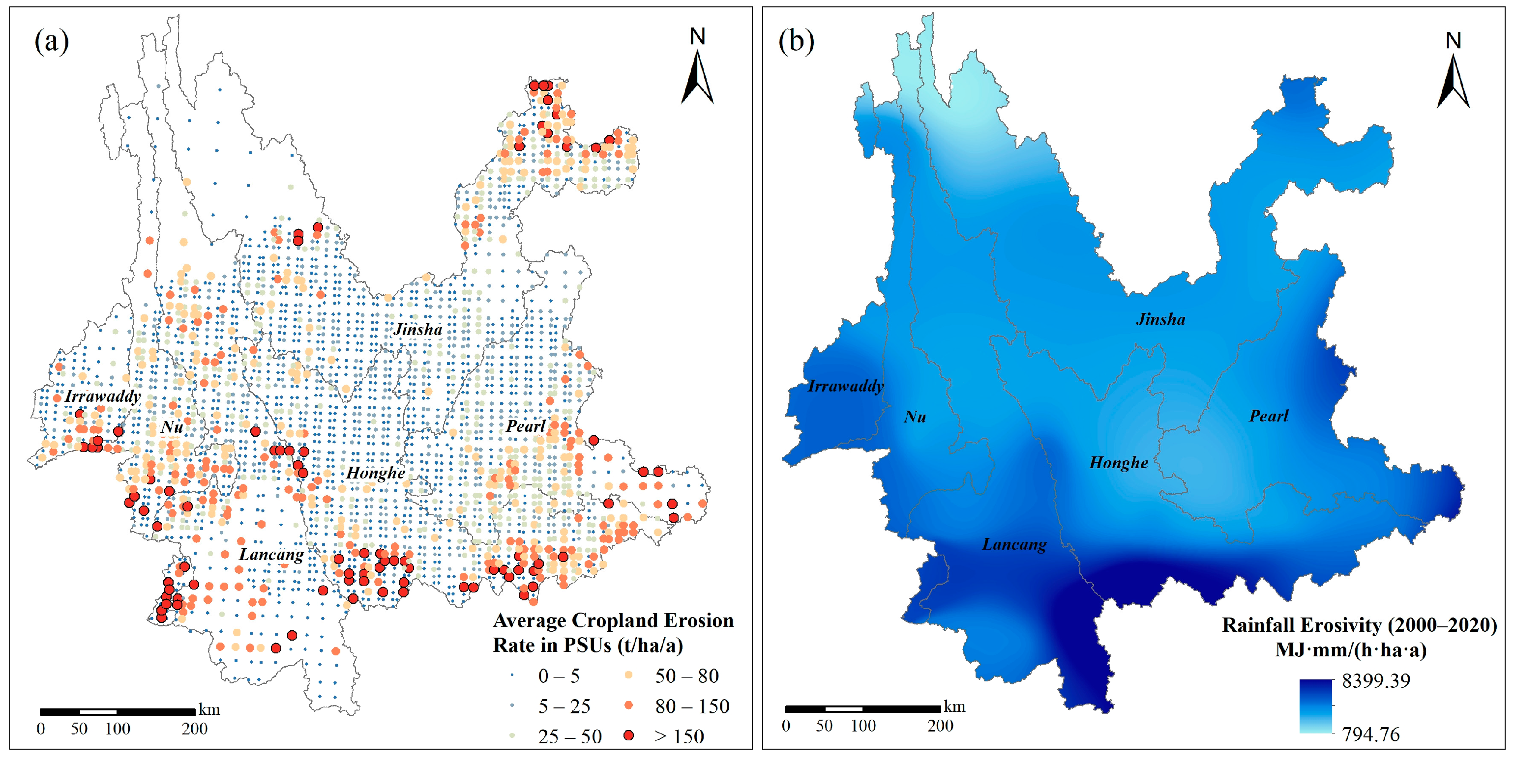
3.1. Soil Erosion Pattern of Yunnan Based on Sampling Survey and Field Investigation

3.1.1. Investigated Land Parcel Basics of Yunnan in the NSES

According to the sampling survey, a total of 20,155 land parcels in 2817 PSUs were investigated on site in Yunnan. The average area of the PSUs was 34.83 ha, and the average patch area of the land parcels was 4.79 ha, which is consistent with the model requirements. The measured mean slope gradient for all the land patches was 20.23°, with a range of 0–82.8°, while the mean slope length was 47.73 m with a range of 0–233.9. The average soil erosion rate of all the land use parcels was 17.02 t/(ha·a). Table 2 lists the basic information on the land parcels of the first-level NLUD-C types. Obviously, in terms of spatial distribution, woodland showed the largest average patch area and number (a total of 10015 land parcels), and was the dominant land use mode in the landscape. The average patch area of cropland was 2.77 ha, and the average slope reached 17.88°, making it very prone to soil erosion.

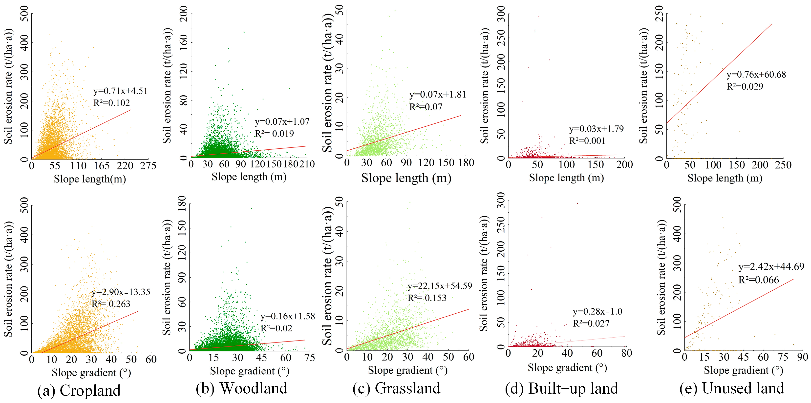
3.1.2. Soil Erosion Rate Variations under Different Land Use Types and Topography

Table 3 lists the various soil erosion factors in the CSLE and the multi-year average soil erosion rates of the NLUD-C second-level land types. Woodland showed a higher average rainfall erosivity than other types, with a value of 3570.37 t·hm2·h/(MJ·hm2·mm), followed by grassland, cropland, built-up land, water bodies and unused land. The highest rainfall erosivity was found in paddy fields and garden plantations (classified as woodland in NLUD-C), as these were mainly distributed in southern Yunnan. Additionally, the lowest lower R values were found on sparse grass and bare land, which are mostly distributed in the northern part of Yunnan and the dry–hot valleys of the six major rivers. Since the main soil types are highly sticky, the K values here were relatively close and small in all regions. In terms of terrain factors, except for built-up land, water bodies, and irrigated land (basically cropland in flat areas with irrigation conditions), all other land types were characterized by high slope steepness and short slopes, and the LS values were generally high for sloping cropland, gardens and unused land. In the CSLE model, the vegetation factor B mainly concerns woodland and grassland. The vegetation coverage of woodland in Yunnan was significantly higher than that of grassland (lower B factor value), while the impact of vegetation on cropland soil erosion has been incorporated into the tillage measure factor T, and intercropping and rotation were here the dominant tillage measures. Out of 6714 cropland parcels investigated, 52.25% of them were adopted with engineering measures. Overall, cropland without ECMs contributed 83.51% of the total soil loss from croplands, with a land area of only 47.75%.
As Yunnan is the only province with a fully plateau–mountainous landscape in China, the impact of terrain on the soil erosion rate is crucial, and it is often the most important factor in water erosion models. With the change of terrain conditions, the soil erosion rates of the five major land use types except water bodies showed varying degrees of difference in different slope gradient and length zones, and soil erosion was found to be much more sensitive to changes in slope steepness than to changes in slope length (Figure 6). For cropland, the average annual soil erosion rate was 40.47t/(ha·a) and the erosion ratio was 70.11% (4707 out of 6714 land parcels with soil erosion rates higher than the soil loss tolerance of 5 t/(ha·a)), far exceeding these values for other land types (28.57% for woodland, 35.42% for grassland, 10.27% for built-up land and 60.53% for unused land). Rain-fed dry land was the main type of cropland (5644 out of 6714 land parcels), with a soil erosion rate of 45.34 t/(ha·a) and erosion ratio of 81.48% (4599 out of 5644 land parcels with soil erosion rates higher than soil loss tolerance), which values are also significantly higher than those of paddy fields and irrigated cropland. For woodland and grassland parcels, higher values were mostly found for sparse vegetation and garden plantations (categorized as woodland but retaining the attributes of cropland). Due to their low coverage and intensive disturbance, high soil erosion rates were mainly found for built-up land in mining areas. Bare soil suffers from some of the highest soil erosion rates among all NLUD-C second-level land types, but it here occupied a small area and did not contribute much to the total soil.
To better present the spatial patterns of cropland erosion rates, we mapped the spatial distribution patterns of cropland erosion rates at the PSU scale (Figure 7a) according to the classification standards of the MWRC. As can be seen from the figure, soil erosion rates in downstream areas of the six major river basins were generally higher than those in upstream areas, and aggregation occurred. Cropland land erosion rates in the central flat area were much lower. Considering the influence of terrain, and similarities in soil properties, planting systems and rotation patterns, the differences can be attributed to the fact that the rainfall erosivity values in the downstream areas were significantly higher than those in the upstream areas (Figure 7a).

3.1.3. Impact of Engineering Conservation Measures on Cropland Soil Erosion

For a long time, scientists and soil conservancy departments have attached great importance to soil conservation in cropland, but with limited data availability, little is known about the effectiveness of engineering conservation measures (ECMs) at large scales. ECMs refer to the measures applied by changing micro terrain conditions to intercept runoff and increase soil infiltration or crop production, such as including a level terrace, a sloping terrace, a fruit tree pit, a check dam, intercepting drains, diversion canals, etc. In the NSES, one of the major tasks is to conduct detailed field surveys on the type, distribution, quantity and area of ECMs. We also quantified the impact of ECMs on soil erosion based on the literature, standard runoff plot observations and data collected under natural or artificial simulated rainfall conditions. To further understand the impacts of ECMs on cropland erosion, we also mapped the spatial distribution of ECMs on PSUs that contain cropland parcels, and analyzed their impact on soil erosion rates at different slope steepness intervals (Figure 8a). Obviously, except for the cultivated areas with flat terrain and low soil erosion rates in the central part, ECMs were spatially distributed throughout the province. The proportion of cropland parcels with ECWs showed a decreasing trend as the slope steepness increased. This was mainly because the large-scale adoption of remediation measures on steep slopes in plateau mountainous regions is difficult, unaffordable and may cause disasters like landslides. Besides this, farmers are more encouraged to return steeply sloping cropland to forest/grassland rather than terraced fields, based on the Grain for Green Policy.
Figure 8b illustrates the effectiveness of soil conservation measures used in mitigating cropland erosion beyond just a reduction in the magnitude of erosion rate. In the sloping cropland in the province, the soil erosion rates of cropland both with and without ECMs increased as the slope gradient increased. Based on field investigations, cropland parcels were found in 1863 out of 2871 PSUs, and the average cropland soil erosion rate for those with ECMs was 12.14 t/(ha·a), while the average cropland soil erosion rate for those without ECMs was 67.25 t/(ha·a). The difference in rates was greater than five-fold, based on the premise that croplands with low erosion rates in their central part were not equipped with ECMs. For steeply sloping zones, this difference was even bigger, reaching a gap of 100 t/(ha·a) in the steepness class of 30–35°, indicating that the effect of ECMS also decreased as the slope gradient increased. Apparently, the allocation of ECMs largely affects the spatial distribution pattern of cropland erosion rates. In terms of soil loss prevention, almost all the croplands in Yunnan demand ECMs to keep the soil erosion within a tolerable rate. However, more attention should be directed towards assessing the difficulty, costs and effectiveness of the treatment (including soil productivity) to determine priority areas where projects should really be adopted.

3.2. Land Use Change Dynamics in Yunnan from 2000 to 2020

Following the update to the NLUD-C data, we optimized the land use change dynamic data for Yunnan from 2000 to 2020. Figure 9 shows the corresponding land use maps for 2000, 2005, 2010, 2015 and 2020. Woodland (67.79–68.44%), cropland (16.56–18.51%) and grassland (10.43–11.64%) were the dominant land types. Woodland could be found in the whole province, while cropland was mainly distributed in the central, northeast and southeast parts, and grassland was concentrated in the Jinsha River Basin and the dry–hot valleys of other river basins. The proportions of water bodies (1.19–1.22%), built-up land (0.82–3.33%) and unused land (0.05–0.06%) were relatively low.
Based on the land use transfer matrix, the land use transformation process and change dynamics from 2000 to 2020 are presented in Figure 10. For the 2000–2005 and 2005–2010 periods, the total land change areas were 1.62 × 10⁴ km2 and 1.73 × 10⁴ km2, respectively, wherein the conversions between cropland and woodland were the dominant changes. For the 2010–2015 and 2015–2020 periods, the total land change areas were 2.06 × 10⁴ km2 and 1.97 × 10⁴ km2, respectively, and the cropland–grassland transformation dominated these periods, while the one-way conversion from cropland to built-up land was also noticeable.
The main LUCC characteristics of Yunnan Province from 2000 to 2020 can be summarized as follows. The built-up land area continued to rise, with a net increase of 9451.57 km2 and a rate of 300.39%. The cropland area continued to decrease, with a net decrease of 7461.83 km2 and a rate of −10.55%. The grassland area continued to decrease, and the net decrease was 4603.39 km2, with a rate of −10.36%. The woodland area increased by 2482.63 km2, but because of the large area base, the change rate was the lowest, at 0.95%. The water bodies and unused land were relatively stable, with increasing areas of 92.75 km2 and 36.75 km2, respectively. Although the change trend of LUCC in each period was relatively consistent, significant differences were also found in region, quantity and main change scenarios. It should be highlighted that the land conversion area related to cropland accounted for 74.02% of all the transformation scenarios, and was the most significant type of land use conversion.
To finally achieve the dynamic quantitative monitoring of cropland erosion rates and soil loss, we analyzed the conversions between cropland and other land types spatially. For each time period, most of the cropland change area was converted to woodland, grassland or built-up land, with lower levels of conversion to water bodies and unused land, while the cropland reclamation area also mostly began as grassland and woodland (Figure 11). Cropland–woodland conversions were mainly found in the river basins of Lancang, Nu, Irrawaddy and southern parts, while cropland–grassland conversions mainly occurred in the Jinsha River Basin and the central grassland–cropland–built-up transition zones. For the past 20 years, the cropland loss areas of the six major river basins can be ordered as Lancang (21.35 km2) > Honghe (13.86 km2) > Nu (13.45 km2) > Pearl (10.76 km2) > Jinsha (9.70 km2) > Irrawaddy (5.50 km2), while the cropland loss ratios can be ordered as Nu (28.76%) > Irrawaddy (22.95%) > Lancang (20.34%) > Honghe (10.20%) > Pearl (5.74%) > Jinsha (4.66%). Apparently, northwestern Yunnan has been suffering serious cropland degradation and loss problems.
As can be seen from Figure 11c, the areas with the largest net decrease in cropland were concentrated in western Yunnan, and mainly distributed in the Irrawaddy River Basin, Nu River Basin and Lancang River Basin. The spatial patterns of the cropland reduction trends in the three river basins were basically consistent with each other. Specifically, a reduction in net cropland from 2000 to 2005 was mainly found in the upper reaches of the basins, but with time, the center of the reduction in net cropland gradually moved from the upstream to the downstream areas. Nearly 90% of the basin area experienced cropland loss. Notably, in the Irrawaddy River Basin, the net decrease was mainly concentrated in the middle and upper reaches before 2015. From 2015 to 2020, the entire basin showed a net decrease in cropland.

3.3. Cropland Soil Erosion Dynamics in Yunnan from 2000 to 2020

In previous work, we optimized the input parameters of the CSLE with the annual average values of vegetation coverage and erosive rainfall data from 2000 to 2020, and recalculated the annual average soil erosion rates for each land type of the PSUs. Since the updated NLUD-C and NSES originated from different programs with different application purposes, the process of land use/cover classification using NLUD-C is much simpler than that using field investigations. Thus, we unified the classification system and retained the six first-level land types of NLUD-C, and determined the average soil erosion rates using an area percentage-weighted average method in PSUs. The high-precision soil erosion rates for different land types in PSUs were further interpolated to the corresponding control areas of PSUs using a nearest neighbor interpolation method. Finally, net soil erosion rates and soil loss changes for different land use conversion scenarios were calculated (Table 4), and then up-to-date dynamic and quantitative soil erosion information on cropland was acquired by incorporation with the revised LUCC dynamics area derived during the past two decades (Figure 12). Considering the average soil erosion rates of each land type, for different LUCC scenarios in Yunnan, we see that cropland change induced increases and decreases in soil erosion rate, and soil loss occurred during the four periods. Conversion from cropland generally reduced the soil erosion intensity, while slope cropland reclamation was the main LUCC type that intensified soil erosion.
Figure 12 presents a representative area located in the Jinsha River Basin. Here, each grid is the control area (grid size of 5 km × 5 km) of a specific Primary Sample Unit. Through sampling surveys, we calculated the multi-year average soil erosion rates of all the land use types in the corresponding grids, as well as the erosion rate changes of various conversion scenarios. It can be seen that both cropland abandonment and expansion occurred in the region, and there was a significant variation in the soil erosion rates for the same LUCC conversion process between grids, despite the fact that they were very close together in geographic distance. During this period, 1.66 km2 and 0.91 km2 of cropland abandonment and expansion, respectively, occurred in the representative area, with the largest area of cropland converted to built-up land, followed by conversion to water bodies. In the dynamic zones, the soil erosion rates caused by different cropland transformation types were also different. Returning cropland to woodland and grassland, and converting cropland to built-up land, reduced the soil erosion rate dramatically.
When the land use type changes, the soil erosion rates and intensity will change accordingly. From 2000 to 2020, as cropland-related LUCC transformations were dominant in the landscape, changes in soil erosion rates and soil loss were also significant in corresponding areas. In the past two decades, the amount of soil loss due to the cropland transfer was −1.28 × 10⁸ t, while the amount of soil loss due to cropland reclamation was 0.96 × 10⁸ t, and the net change in soil erosion caused by cropland transformations was −0.32 × 10⁸ t, with a decrease ratio of 12.12% of the total cropland soil loss (Figure 13).
The cropland area continued to decline over the following two decades, and most of it was converted into woodland, grassland or built-up land. The conversions from cropland to woodland and grassland accounted for the greatest proportions of cropland erosion reduction, at 43.75% and 34.64%, respectively. The conversion from cropland to built-up land accounted for 21.36% of the reduction. Conversion from cropland to woodland has also been a major contributor to the decline in soil erosion in cropland areas. As for the increase in soil erosion, about 99% of it was caused by cropland reclamation, and conversion from grassland to cropland contributed 56.18% of the total increase in soil erosion.
The conversions between cropland and other land uses also had different effects on the quantity of soil erosion in different periods. Among these, compared with mutual conversions between woodland and grassland, the conversion between cropland and built-up land more often represented a unidirectional change. Due to the larger size of the net change area, the net reduction in erosion caused by cropland to built-up land conversion was also the largest, and the cropland–built-up land change scenario accounted for nearly 40% of the total reduction in soil erosion during the 2010–2015 period, as this was also the period with the fastest urbanization speed. For the four periods of 2000–2005, 2005–2010, 2010–2015 and 2015–2020, the mutual conversions between cropland and woodland were relatively stable. Most of the soil erosion reduction caused by the conversion from cropland to grassland was concentrated in 2010–2020, while the increase in soil erosion caused by conversion from grassland to cropland showed a decreasing trend year by year.

4. Discussion

The constant measurement and observation of soil erosion rates at large scales have proven to be extremely challenging and unrealistic. Based on field sampling surveys, the CSLE model and LUCC data, we proposed a rapid monitoring method to extrapolate cropland soil erosion rates and soil loss from point to surface in mountainous areas. The 20,155 investigated land parcels showed the same data quality, and all of them met the requirements of USLE-type empirical models in size and scale (less than 150 ha). The LUCC data were further improved using a non-homologous data voting method, with steps of accuracy assessment, consistency analysis and standardization of the classification system. To facilitate decision-making, we provided continuous distribution information on cropland erosion rates, hotspots and soil loss amounts. The soil erosion rates of each land type were in good agreement with the values reported in the literature [6,30]. Apparently, when choosing a soil erosion model, one should pay more attention to the model’s strengths, limitations and application scope. If the input data do not meet the requirements, the results produced by over-parameterization and scaling extrapolation are often less reliable than those given by a simple model.
Under climate change and land use change scenarios, cropland erosion and degradation are a mutually promoting process. In areas with extremely high biodiversity like Yunnan, the implementation of policies such as returning farmland to forest/grass is of great value in relation to controlling soil erosion and protecting habitats and biodiversity. However, our research shows that a cropland area of 7461.83 km2 (−10.55%) has vanished during the past 20 years, which is an extremely shocking figure, and the originally small cropland area per head of population is continuing to shrink. Furthermore, the newly reclaimed slope lands are often accompanied with severe soil erosion rates, directly threatening local food security. The real threat that should be noted here is that more and more land is becoming unfarmable due to high soil erosion rates. It is estimated that if the current soil erosion rate in China continues, food production will decrease by 40% in the next 50 years. Moreover, the rising global population demands the intensification of agricultural production to meet food demand, which is expected to increase by 50% in 2030, possibly doubling by 2050 [1]. If the current population growth speed and soil erosion rates continue unchecked, humankind may eventually lose the ability to feed itself in the future, barring unforeseen scientific advances [5]. The regulation of sloping croplands is extremely difficult in mountainous areas, as the croplands are distributed in a fragmented manner on steep slopes. According to local statistics [86], the annual average cropland land area subjected to newly developed erosion control measures in Yunnan is 31.69 km2. It will take more than 1000 years and CNY 180 billion to complete the regulation of unmeasured sloping cropland, and this is assuming that each cropland area can be managed without considering the difficulties of governance. Considering the cropland loss speed, urgent action is needed to face the threat of cropland soil erosion; we must develop a shared understanding via collaboration among stakeholders and those in different roles (e.g., scientists, governments, farmers and environmentalists).
Field observations of soil erosion are always closer to the truth than modeling results and thus constitute the most vital part of scientific investigation. However, due to the high cost of construction and monitoring of standard runoff plots, most regions around the world face the problem of an under-representation of observational data, especially in large mountainous areas of developing countries with poor economic conditions, so full-coverage real erosion measurements validation is challenging despite we have made some validation for specific land use types like grasslands [80] and orchards [81] in certain places. Currently, remote sensing is instrumental for investigating, evaluating, monitoring and understanding the spatial extent and rate of soil erosion due to the advantages of its large coverage area and short revisit period. High-resolution imagery provides high-quality data and thus raises fewer uncertainties in soil erosion mapping, but its utility remains hindered due to the acquisition costs. As the spatial, hyperspectral and temporal resolution continuously increase, this technology sheds more and more light on small-scale heterogeneity, and most of the limitations of large-scale soil erosion modeling may eventually be resolved in the future. With a robust framework of samples with high density, using remote sensing in large-scale dynamic soil erosion mapping and monitoring will be very promising.
We proposed a combination method of point (PSUs) and surface (LUCC data) approaches for quantitative soil erosion assessments in a large region; the work depended greatly on the collection of detailed data in the field. The NSES was the first ever national soil erosion investigation undertaken using field investigations, thus ensuring the accuracy of the input data. However, the quality and representativeness of the data for areas with low sampling density and missing sample information require further evaluation.

5. Conclusions

Long-term, quantitative information on large-scale cropland erosion rates is vital for agricultural planning and management, but has long been hindered by data availability and model limitations. Taking the CSLE as a monitoring tool, by integrating a large number of field sampling surveys and LUCC remote sensing data into national surveys, we here proposed a long-term time series dynamic method for monitoring cropland soil erosion rates and soil losses, and we conducted application research in the Yunnan Plateau, featuring complex terrain conditions. Differently from previous studies, this study was conducted based on a large number of field surveys and remote sensing to improve the model’s input data and reduce uncertainties. The results show the following:
(1)
The average soil erosion rate and erosion ratio of cropland are significantly higher than those of other land use types, and huge spatial differences in erosion were found within each land use type. In addition, soil erosion rates are generally more sensitive to slope than slope length for all land use types. The soil conservation measures adopted in croplands are highly effective in controlling soil erosion, and they can change the spatial pattern of soil erosion significantly.
(2)
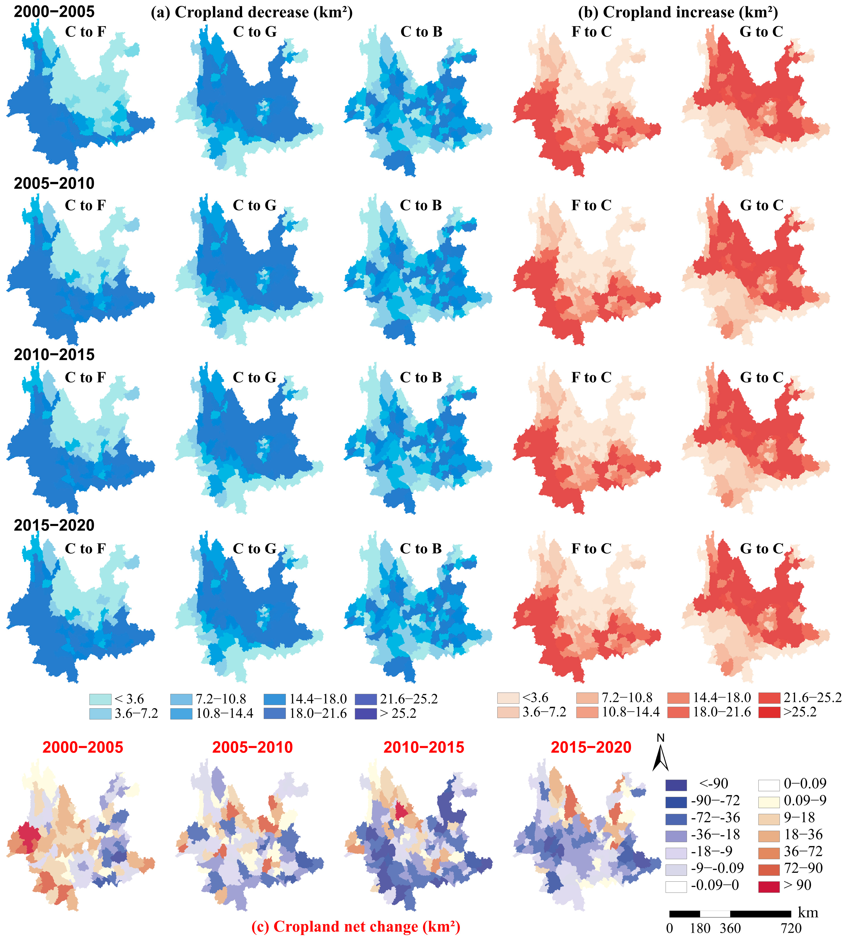
In the past 20 years, due to the Grain for Green Policy, population growth and rapid urbanization expansion, the areas of cropland and grassland in Yunnan have continued to decrease, with the reduction ratios both exceeding 10%, while the area of built-up impervious land has increased by 300%. The conversions between cropland and grassland were mainly concentrated in the Jinsha River Basin and northern parts, while the conversion between cropland and woodland was widely distributed throughout the province, especially in the southern region. Cropland-related conversions accounted for 74.02% of all LUCC scenarios and showed significantly different transformation intensities for each period.
(3)
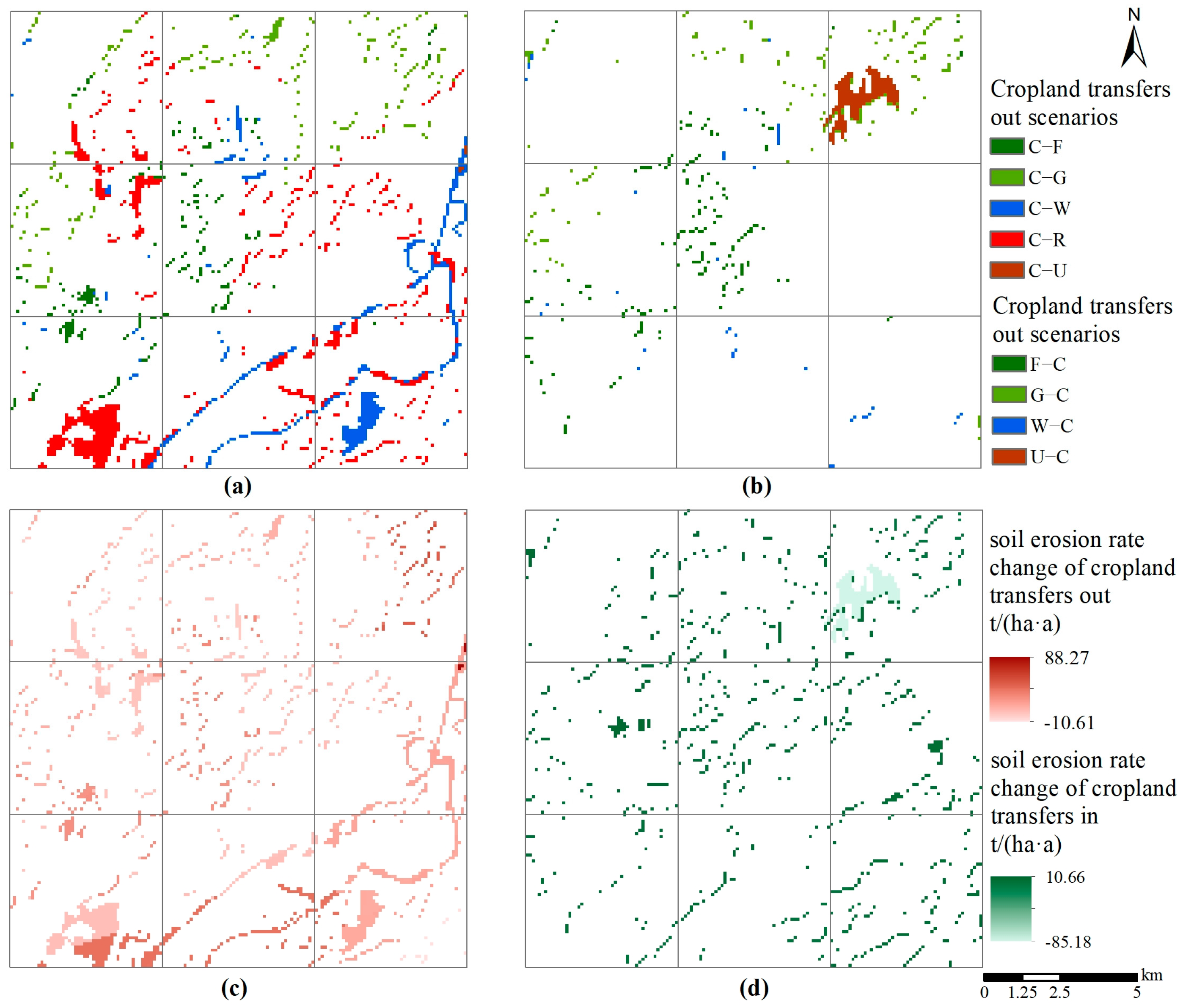
Significant changes in land use at the landscape scale have huge impacts on cropland erosion in Yunnan. During 2000–2020, the amount of cropland soil loss decreased by 0.32 × 10⁸ t, with a decrease rate of 12.12%. The net soil loss change varied significantly in the six major river basins in different periods and LUCC scenarios. Excluding the reclamation of cropland in the lower reaches of river basins and southern Yunnan, which induced a large increase in net soil loss, soil erosion in other areas was significantly reduced due to the sharp reduction in cropland area. This is the first long-term quantitative study of cropland soil erosion in this area, featuring multiple national investigations, and it is of great significance for understanding the soil erosion patterns of cropland and clarifying the directions and focus of prevention activities, as well as protecting precious cropland resources to ensure food security in mountainous areas.

Author Contributions

Conceptualization, methodology, funding acquisition, G.C.; data curation, software, writing—original draft preparation, formal analysis, visualization, J.Z.; supervision, B.T.; date collection, review and editing, X.D.; visualization, L.Z.; data processing, resources, X.W.; investigation, validation, Q.G. All authors have read and agreed to the published version of the manuscript.

Funding

This research was funded by the Basic Research Project of Yunnan Province (Grant No. 202401AT070366, Grant No. 202101AU070161) and the Strategic Priority Research Program of Chinese Academy of Sciences, Grant No. XDA26050301-01).

Data Availability Statement

The data used in this study are available upon request.

Acknowledgments

Thanks are due to the field data gatherers in the National Soil Erosion Survey.

Conflicts of Interest

The authors declare no conflicts of interest.

References

  1. Banwart, S. Save our soils. Nature 2011, 474, 151–152. [Google Scholar] [CrossRef]
  2. Banwart, S.A.; Nikolaidis, N.P.; Zhu, Y.G. Soil functions: Connecting earth’s critical zone. Annu. Rev. Earth Planet. Sci. 2019, 47, 333–359. [Google Scholar] [CrossRef]
  3. Lehmann, J.; Bossio, D.A.; Kögel-Knabner, I. The concept and future prospects of soil health. Nat. Rev. Earth Environ. 2020, 1, 544–553. [Google Scholar] [CrossRef]
  4. Borrelli, P.; Robinson, D.A.; Fleischer, L.R. An assessment of the global impact of 21st century land use change on soil erosion. Nat. Commun. 2017, 8, 2013. [Google Scholar] [CrossRef]
  5. Ascough, J.C.; Flanagan, D.C.; Tatarko, J. Soil erosion modeling and conservation planning. In Precision Conservation: Geospatial Techniques for Agricultural and Natural Resources Conservation; John Wiley Sons: Hoboken, NJ, USA, 2017; pp. 1–25. [Google Scholar]
  6. Wuepper, D.; Borrelli, P.; Finger, R. Countries and the global rate of soil erosion. Nat. Sustain. 2020, 3, 51–55. [Google Scholar] [CrossRef]
  7. Montgomery, D.R. Soil erosion and agricultural sustainability. Proc. Natl. Acad. Sci. USA 2007, 104, 13268–13272. [Google Scholar] [CrossRef]
  8. Morgan, R.P.C. Soil Erosion and Conservation; John Wiley Sons: Hoboken, NJ, USA, 2009; pp. 15–22. [Google Scholar]
  9. Boardman, J. How much is soil erosion costing us? Geography 2021, 106, 32–38. [Google Scholar] [CrossRef]
  10. Wang, Z.; Hoffmann, T.; Six, J. Human-induced erosion has offset one-third of carbon emissions from land cover change. Nat. Clim. Chang. 2017, 7, 345–349. [Google Scholar] [CrossRef]
  11. Alewell, C.; Ringeval, B.; Ballabio, C. Global phosphorus shortage will be aggravated by soil erosion. Nat. Commun. 2020, 11, 4546. [Google Scholar] [CrossRef]
  12. Li, J.; Xiong, M.; Sun, R. Temporal variability of global potential water erosion based on an improved USLE model. Int. Soil Water Conserv. Res. 2024, 12, 1–12. [Google Scholar] [CrossRef]
  13. Borrelli, P.; Ballabio, C.; Yang, J.E. GloSEM: High-resolution global estimates of present and future soil displacement in croplands by water erosion. Sci. Data 2022, 9, 406. [Google Scholar] [CrossRef]
  14. Shanshan, W.; Baoyang, S.; Chaodong, L. Runoff and soil erosion on slope Cropland: A Review. J. Resour. Ecol. 2018, 9, 461–470. [Google Scholar] [CrossRef]
  15. Pimentel, D.; Burgess, M. Soil erosion threatens food production. Agriculture 2013, 3, 443–463. [Google Scholar] [CrossRef]
  16. Xiong, M.; Sun, R.; Chen, L. A global comparison of soil erosion associated with land use and climate type. Geoderma 2019, 343, 31–39. [Google Scholar] [CrossRef]
  17. Boardman, J. Soil erosion science: Reflections on the limitations of current approaches. Catena 2006, 68, 73–86. [Google Scholar] [CrossRef]
  18. De, V.J.; Poesen, J.; Verstraeten, G. Predicting soil erosion and sediment yield at regional scales: Where do we stand? Earth-Sci. Rev. 2013, 127, 16–29. [Google Scholar]
  19. Vrieling, A. Satellite remote sensing for water erosion assessment: A review. Catena 2006, 65, 2–18. [Google Scholar] [CrossRef]
  20. Alewell, C.; Borrelli, P.; Meusburger, K. Using the USLE: Chances, challenges and limitations of soil erosion modelling. Int. Soil Water Conserv. Res. 2019, 7, 203–225. [Google Scholar] [CrossRef]
  21. Laflen, J.M.; Flanagan, D.C. The development of US soil erosion prediction and modeling. Int. Soil Water Conserv. Res. 2013, 1, 1–11. [Google Scholar] [CrossRef]
  22. Xie, Y.; Zhao, Y.; Zhang, Y. History and current situation of soil erosion survey in the United States. Soil Water Conserv. China 2013, 10, 53–60. [Google Scholar]
  23. Borrelli, P.; Alewell, C.; Alvarez, P. Soil erosion modelling: A global review and statistical analysis. Sci. Total Environ. 2021, 780, 146494. [Google Scholar] [CrossRef]
  24. Olson, K.R.; Gennadiyev, A.N.; Zhidkin, A.P. Use of magnetic tracer and radio-cesium methods to determine past cropland soil erosion amounts and rates. Catena 2013, 104, 103–110. [Google Scholar] [CrossRef]
  25. Renard, K.G. Predicting Soil Erosion by Water: A Guide to Conservation Planning with the Revised Universal Soil Loss Equation (RUSLE); US Department of Agriculture, Agricultural Research Service: Washington, DC, USA, 1997; p. 234.
  26. Flanagan, D.C.; Gilley, J.E.; Franti, T.G. Water Erosion Prediction Project (WEPP): Development history, model capabilities, and future enhancements. Trans. ASABE 2007, 50, 1603–1612. [Google Scholar] [CrossRef]
  27. Guo, Y.; Peng, C.; Zhu, Q. Modelling the impacts of climate and land use changes on soil water erosion: Model applications, limitations and future challenges. J. Environ. Manag. 2019, 250, 109403. [Google Scholar] [CrossRef]
  28. Benavidez, R.; Jackson, B.; Maxwell, D. A review of the (Revised) Universal Soil Loss Equation ((R) USLE): With a view to increasing its global applicability and improving soil loss estimates. Hydrol. Earth Syst. Sci. 2018, 22, 6059–6086. [Google Scholar] [CrossRef]
  29. Xie, Y.; Yue, Y.T. Application of soil erosion models for soil and water conservation. Sci. Soil Water Conserv. 2018, 16, 25–37. (In Chinese) [Google Scholar]
  30. García-Ruiz, J.M.; Beguería, S.; Nadal-Romero, E. A meta-analysis of soil erosion rates across the world. Geomorphology 2015, 239, 160–173. [Google Scholar] [CrossRef]
  31. Rompaey, A.J.J.V.; Govers, G. Data quality and model complexity for regional scale soil erosion prediction. Int. J. Geogr. Inf. Sci. 2002, 16, 663–680. [Google Scholar] [CrossRef]
  32. Liu, B.Y.; Guo, S.Y.; Li, Z.G.; Xie, Y.; Zhang, K.L.; Liu, X.C. Sampling survey of water erosion in China. Soil Water Conserv. China 2013, 1, 26–34. (In Chinese) [Google Scholar]
  33. Liu, B.Y.; Xie, Y.; Li, Z.G.; Liang, Y.; Zhang, W.B.; Fu, S.H.; Yin, S.Q.; Wei, X.; Zhang, K.L.; Wang, Z.Q. The assessment of soil loss by water erosion in China. Int. Soil Water Conserv. Res. 2020, 8, 430–439. [Google Scholar] [CrossRef]
  34. Nusser, S.M.; Goebel, J.J. The National Resources Inventory: A long-term multi-resource monitoring programme. Environ. Ecol. Stat. 1997, 4, 181–204. [Google Scholar] [CrossRef]
  35. Matthews, F.; Verstraeten, G.; Borrelli, P. EUSEDcollab: A network of data from European catchments to monitor net soil erosion by water. Sci. Data 2023, 10, 515. [Google Scholar] [CrossRef]
  36. Borrelli, P.; Poesen, J.; Vanmaercke, M. Monitoring gully erosion in the European Union: A novel approach based on the Land Use/Cover Area frame survey (LUCAS). Int. Soil Water Conserv. Res. 2022, 10, 17–28. [Google Scholar] [CrossRef]
  37. Sepuru, T.K.; Dube, T. An appraisal on the progress of remote sensing applications in soil erosion mapping and monitoring. Remote Sens. Appl. Soc. Environ. 2018, 9, 1–9. [Google Scholar] [CrossRef]
  38. Wang, J.; Zhen, J.; Hu, W. Remote sensing of soil degradation: Progress and perspective. Int. Soil Water Conserv. Res. 2023, 11, 429–454. [Google Scholar] [CrossRef]
  39. Yang, Y.; Shi, Y.; Liang, X. Evaluation of structure from motion (SfM) photogrammetry on the measurement of rill and inter-rill erosion in a typical loess. Geomorphology 2021, 385, 107734. [Google Scholar] [CrossRef]
  40. Fenta, A.A.; Tsunekawa, A.; Haregeweyn, N. Improving satellite-based global rainfall erosivity estimates through merging with gauge data. J. Hydrol. 2023, 620, 129555. [Google Scholar] [CrossRef]
  41. Chen, Y.; Xu, M.; Wang, Z. Applicability of two satellite-based precipitation products for assessing rainfall erosivity in China. Sci. Total Environ. 2021, 757, 143975. [Google Scholar] [CrossRef]
  42. Angelopoulou, T.; Tziolas, N.; Balafoutis, A. Remote sensing techniques for soil organic carbon estimation: A review. Remote Sens. 2019, 11, 676. [Google Scholar] [CrossRef]
  43. Roering, J.J.; Stimely, L.L.; Mackey, B.H. Using DInSAR, airborne LiDAR, and archival air photos to quantify landsliding and sediment transport. Geophys. Res. Lett. 2009, 36, L19402. [Google Scholar] [CrossRef]
  44. Fendrich, A.N.; Matthews, F.; Van Eynde, E. From regional to parcel scale: A high-resolution map of cover crops across Europe combining satellite data with statistical surveys. Sci. Total Environ. 2023, 873, 162300. [Google Scholar] [CrossRef]
  45. Feng, Q.; Zhao, W.W. The study on cover-management factor in USLE and RUSLE: A review. Acta Ecol. Sin. 2014, 34, 4461–4472. [Google Scholar]
  46. Ebabu, K.; Tsunekawa, A.; Haregeweyn, N. Global analysis of cover management and support practice factors that control soil erosion and conservation. Int. Soil Water Conserv. Res. 2022, 10, 161–176. [Google Scholar] [CrossRef]
  47. Panagos, P.; Borrelli, P.; Meusburger, K. Modelling the effect of support practices (P-factor) on the reduction of soil erosion by water at European scale. Environ. Sci. Policy 2015, 51, 23–34. [Google Scholar] [CrossRef]
  48. Zhao, H.; Fang, X.; Ding, H. Extraction of terraces on the Loess Plateau from high-resolution DEMs and imagery utilizing object-based image analysis. ISPRS Int. J. Geo-Inf. 2017, 6, 157. [Google Scholar] [CrossRef]
  49. Duan, X.; Rong, L.; Bai, Z. Effects of soil conservation measures on soil erosion in the Yunnan Plateau, southwest China. J. Soil Water Conserv. 2020, 75, 131–142. [Google Scholar] [CrossRef]
  50. Duan, X.; Bai, Z.; Rong, L. Investigation method for regional soil erosion based on the Chinese Soil Loss Equation and high-resolution spatial data: Case study on the mountainous Yunnan Province, China. Catena 2020, 184, 104237. [Google Scholar] [CrossRef]
  51. Panos, P.; Pasquale, B.; Jean, P. The new assessment of soil loss by water erosion in Europe. Environ. Sci. Policy 2015, 8, 438–447. [Google Scholar]
  52. Panagos, P.; Meusburger, K.; Van Liedekerke, M. Assessing soil erosion in Europe based on data collected through a European network. Soil Sci. Plant Nutr. 2014, 60, 15–29. [Google Scholar] [CrossRef]
  53. Duan, X.; Tao, Y.; Bai, Z. Regional Soil Erosion Survey Methods; Science Press: Beijing, China, 2019; pp. 111–123. [Google Scholar]
  54. Yin, S.; Zhu, Z.; Wang, L. Regional soil erosion assessment based on a sample survey and geostatistics. Hydrol. Earth Syst. Sci. 2018, 22, 1695–1712. [Google Scholar] [CrossRef]
  55. Xie, Y.; Lin, H.; Ye, Y. Changes in soil erosion in cropland in northeastern China over the past 300 years. Catena 2019, 176, 410–418. [Google Scholar] [CrossRef]
  56. Borrelli, P.; Robinson, D.A.; Panagos, P. Land use and climate change impacts on global soil erosion by water (2015–2070). Proc. Natl. Acad. Sci. USA 2020, 117, 21994–22001. [Google Scholar] [CrossRef]
  57. Kidane, M.; Bezie, A.; Kesete, N. The impact of land use and land cover (LULC) dynamics on soil erosion and sediment yield in Ethiopia. Heliyon 2019, 5, e02981. [Google Scholar] [CrossRef]
  58. Brandolini, F.; Kinnaird, T.C.; Srivastava, A. Modelling the impact of historic landscape change on soil erosion and degradation. Sci. Rep. 2023, 13, 4949. [Google Scholar] [CrossRef]
  59. Chalise, D.; Kumar, L. Land use change affects water erosion in the Nepal Himalayas. PLoS ONE 2020, 15, e0231692. [Google Scholar] [CrossRef]
  60. Zhang, Z.; Zhao, X. Remote Sensing Monitoring of Land Use in China; Planet Mapping Press: Beijing, China, 2012; pp. 99–103. [Google Scholar]
  61. Wang, X.; Zhao, X.; Zhang, Z. Assessment of soil erosion change and its relationships with land use/cover change in China from the end of the 1980s to 2010. Catena 2016, 137, 256–268. [Google Scholar] [CrossRef]
  62. Xi, J.; Zhao, X.; Wang, X. Assessing the impact of land use change on soil erosion on the Loess Plateau of China from the end of the 1980s to 2010. J. Soil Water Conserv. 2017, 72, 452–462. [Google Scholar] [CrossRef]
  63. Nearing, M.A.; Xie, Y.; Liu, B. Natural and anthropogenic rates of soil erosion. Int. Soil Water Conserv. Res. 2017, 5, 77–84. [Google Scholar] [CrossRef]
  64. Baoyuan, L.; Keli, Z.; Yun, X. An empirical soil loss equation. In Proceedings of the 12th International Soil Conservation Organization Conference, Beijing, China, 26 May 2002; pp. 26–31. [Google Scholar]
  65. Chen, G.; Zhang, Z.; Guo, Q. Quantitative assessment of soil erosion based on CSLE and the 2010 national soil erosion survey at regional scale in Yunnan Province of China. Sustainability 2019, 11, 3252. [Google Scholar] [CrossRef]
  66. Thomas, A. The onset of the rainy season in Yunnan province, PR China and its significance for agricultural operations. Int. J. Biometeorol. 1993, 37, 170–176. [Google Scholar] [CrossRef]
  67. Li, Y.G.; He, D.; Hu, J.M. Variability of extreme precipitation over Yunnan Province, China 1960–2012. Int. J. Climatol. 2015, 35, 245–258. [Google Scholar] [CrossRef]
  68. Sun, H.; Wang, J.; Xiong, J. Vegetation change and its response to climate change in Yunnan Province, China. Adv. Meteorol. 2021, 2021, 8857589. [Google Scholar] [CrossRef]
  69. Guo, S.Y.; Liu, B.Y. Soil Erosion Investigation and Evaluation; China Water Resources and Hydropower Press: Beijing, China, 2014; pp. 63–70. (In Chinese) [Google Scholar]
  70. Zhang, Z.; Wang, X.; Zhao, X. A 2010 update of National Land Use/Cover Database of China at 1: 100000 scale using medium spatial resolution satellite images. Remote Sens. Environ. 2014, 149, 142–154. [Google Scholar] [CrossRef]
  71. Liu, L.; Zhang, X.; Chen, X. GLC_FCS30-2020: Global Land Cover with Fine Classification System at 30 m in 2020. Earth Syst. Sci. Data 2020, 13, 2753–2776. [Google Scholar]
  72. Yang, J.; Huang, X. The 30 m annual land cover dataset and its dynamics in China from 1990 to 2019. Earth Syst. Sci. Data 2021, 13, 3907–3925. [Google Scholar] [CrossRef]
  73. Chen, J.; Chen, J.; Liao, A. Global land cover mapping at 30 m resolution: A POK-based operational approach. ISPRS J. Photogramm. Remote Sens. 2015, 103, 7–27. [Google Scholar] [CrossRef]
  74. Karra, K.; Kontgis, C.; Statman-Weil, Z. Global land use/land cover with Sentinel 2 and deep learning. In Proceedings of the 2021 IEEE International Geoscience and Remote Sensing Symposium IGARSS, Brussels, Belgium, 11–16 July 2021; pp. 4704–4707. [Google Scholar]
  75. Zanaga, D.; Van, D.K.R.; Daems, D. ESA WorldCover 10 m 2021 v200. Land 2022, 12, 1740. [Google Scholar]
  76. Liu, Y.; Zhong, Y.; Ma, A. Cross-resolution national-scale land-cover mapping based on noisy label learning: A case study of China. Int. J. Appl. Earth Obs. Geoinf. 2023, 118, 103265. [Google Scholar] [CrossRef]
  77. Brown, C.F.; Brumby, S.P.; Guzder-Williams, B. Dynamic World, Near real-time global 10 m land use land cover mapping. Sci. Data 2022, 9, 251. [Google Scholar] [CrossRef]
  78. Shi, W.; Huang, M.; Barbour, S.L. Storm-based CSLE that incorporates the estimated runoff for soil loss prediction on the Chinese Loess Plateau. Soil Tillage Res. 2018, 180, 137–147. [Google Scholar] [CrossRef]
  79. Zhu, Y.; Zhang, W.B.; Liu, S.H. A batch computation method of soil erosion modulus in the Frist National Water Conservancy Survey-Design and application of water erosion modulus calculator based on CSLE and GIS. Bull. Soil Water Conserv. 2012, 32, 291–295. (In Chinese) [Google Scholar]
  80. Chen, G.; Wang, Y.; Wen, Q. An Erosion-Based Approach Using Multi-Source Remote Sensing Imagery for Grassland Restoration Patterns in a Plateau Mountainous Region, SW China. Remote Sens. 2023, 15, 2047. [Google Scholar] [CrossRef]
  81. Tan, R.; Chen, G.; Tang, B. Landscape Pattern of Sloping Garden Erosion Based on CSLE and Multi-Source Satellite Imagery in Tropical Xishuangbanna, Southwest China. Remote Sens. 2023, 15, 5613. [Google Scholar] [CrossRef]
  82. Lu, S.; Duan, X.; Wei, S. An insight to calculate soil conservation service. Geogr. Sustain. 2022, 3, 237–245. [Google Scholar] [CrossRef]
  83. Liu, B.Y.; Nearing, M.A.; Risse, L.M. Slope gradient effects on soil loss for steep slopes. Trans. ASAE 1994, 37, 1835–1840. [Google Scholar] [CrossRef]
  84. Stehman, S.V.; Foody, G.M. Key issues in rigorous accuracy assessment of land cover products. Remote Sens. Environ. 2019, 231, 111199. [Google Scholar] [CrossRef]
  85. Yuan, Y.; Wen, Q.; Zhao, X.; Liu, S.; Zhu, K.; Hu, B. Identifying Grassland Distribution in a Mountainous Region in Southwest China Using Multi-Source Remote Sensing Images. Remote Sens. 2022, 14, 1472. [Google Scholar] [CrossRef]
  86. Wang, W.; He, L.S. Survey and analysis on current situation of slope farmland in Yunnan province. J. Soil Water Conserv. 2019, 5, 20–23. (In Chinese) [Google Scholar]
Figure 1. Map of Yunnan Province showing the six major rivers, basins and cities, and the elevation variation.
Remotesensing 16 00977 g001
Figure 2. (a) A spatial representation of the sampling design and grid division scheme; (b) soil and water conservation regionalization map of China based on erosive forces; (c) Primary Sample Units (PSUs) allocated in Yunnan Province in the National Soil Erosion Survey (NSES) in China; (d) distribution of corresponding PSUs with different sampling densities and investigation goals in the NSES.
Remotesensing 16 00977 g002
Figure 3. (a) Framework for calculating soil erosion modulus of PSUs using the CSLE model; (b) a random example of field-derived PSU and layers of detailed soil erosion information (factors and rates, resolution 10 m).
Remotesensing 16 00977 g003
Figure 4. Data optimization process using the non-homologous data voting method and multi-source LUCC datasets in this study.
Remotesensing 16 00977 g004
Figure 5. Comparison of three other time series land use products and our revised NLUD-C result for different scenes (ae) using high-resolution images.
Remotesensing 16 00977 g005
Figure 6. Relationship between topographical factors and soil erosion modulus of each land type.
Remotesensing 16 00977 g006
Figure 7. (a) Soil erosion rates of cropland in PSUs; (b) average annual rainfall erosivity of Yunnan during 2000–2020.
Remotesensing 16 00977 g007
Figure 8. (a) Cropland PSUs with and without engineering measures; (b) soil erosion rate of cropland with and without engineering measures.
Remotesensing 16 00977 g008
Figure 9. Optimized land use maps of Yunnan from 2000 to 2020.
Remotesensing 16 00977 g009
Figure 10. Land use transfer process and change dynamics in Yunnan from 2000 to 2020.
Remotesensing 16 00977 g010
Figure 11. Spatial distribution of cropland conversions and net changes at the county level in Yunnan. Notes: C—cropland; F—forestland; G—grassland; B—built-up.
Remotesensing 16 00977 g011
Figure 12. Calculation process of net soil erosion change caused by the transformations of cropland. (a) Cropland transfers out scenarios; (b) cropland transfers in scenarios; (c) soil erosion rate change of cropland transfers out; (d) soil erosion rate change of cropland transfers in.
Remotesensing 16 00977 g012
Figure 13. (a) Quantities and (b) spatial patterns of soil loss induced by cropland transformations in Yunnan during 2000–2020.
Remotesensing 16 00977 g013
Table 1. Details of the publicly accessible non-homogeneous LUCC datasets used.
DatasetsImage SourceMethodCoverResolutionOA
NLUD-CLandsat TM/ETMInteractive interpretationChina30 m>90%
GLC_FCS30Landsat TM/ETM/OLIRandom forestGlobal30 m82.5%
CLCDLandsat TM/ETM/OLISupervisory algorithmChina30 m79.31%
GlobeLand30Landsat/HJ-1/GF-1POK methodGlobal30 m85.72%
ESRI_LCSentinel-2Deep learningGlobal10 m85%
ESA_WCSentinel-2Random forestGlobal10 m75%
CRLCSentinel-2Deep learningChina10 m84%
Dynamic WorldSentinel-2Deep learningGlobal10 m72%
Table 2. Land parcel basic information for the PSUs in Yunnan in the National Soil Erosion Survey.
First-Level TypesNPAPAMax-PAMin-PAASGASLSEMSEM Range
Number%
Cropland671433.312.7781.920.0217.8847.9440.470–428.95
Woodland10,01549.697.0386.530.0322.7948.625.370–174.12
Grassland17428.643.0573.160.0220.8447.855.160–49.70
Water bodies2571.281.3418.560.034.1421.28
Built-up land12376.141.3325.010.0114.0242.962.950–293.67
Unused land1900.942.5041.960.0419.0544.9496.520–455.15
Notes: NP, number of patches; APA, average parcel area (ha); Max-PA, max parcel area (ha); Min-PA, min parcel area (ha); ASG, average slope steepness (°); ASL, average slope length (m); SEM, soil erosion modulus (t/(ha·a)).
Table 3. Soil erosion rates and factors of NLUD-C land types at parcel scale based on investigation.
NLUD-C Land TypesRKLSBETA
First-LevelSecond-Level
CroplandDryland3343.940.0061.485.6910.690.3345.34
Paddy fields3898.490.0051.254.3710.020.401.61
Irrigated land2681.280.0061.152.1710.510.277.80
WoodlandForest3485.290.0061.563.960.03113.61
Shrub3270.270.0061.574.160.04114.68
Sparse woods3378.440.0051.553.730.120.96114.48
Gardens3825.290.0061.526.420.050.770.986.65
GrasslandDense grass3569.070.0061.483.510.050.9714.89
Moderate grass3218.250.0061.493.620.060.9715.72
Sparse grass3029.180.0051.523.790.060.9715.87
Water bodies3147.590.982.06011
Built-up landRural3249.220.0061.404.570.020.211.18
Urban3200.180.0060.910.710.010.0911.20
Mining land3271.480.0051.393.810.950.14118.21
Unused landBare soil2945.280.0061.475.9010.981156.73
Bare rock3017.590.0061.476.2100.9810
Notes: R, MJ·mm/(hm2·h·a); K, t·hm2·h/(MJ·hm2·mm); L, S, B, E, T, dimensionless; A, t/(hm2·a).
Table 4. Soil erosion rate changes under different LUCC scenarios in the six major river basins.
LUCC ScenariosHongheIrrawaddyJinshaLancangNuPeal
C to F−46.02−31.72−24.63−65.22−52.90−28.80
C to G−44.82−29.02−23.12−64.31−48.91−28.53
C to W−50.12−34.53−29.17−69.95−57.06−33.12
C to R−43.23−28.16−27.72−66.53−55.72−29.27
C to U64.02101.1163.2393.83115.6254.69
Notes: unit, t/(ha·a); C—cropland; F—forestland; G—grassland; W—water; R—residential land; U—unused land.
Disclaimer/Publisher’s Note: The statements, opinions and data contained in all publications are solely those of the individual author(s) and contributor(s) and not of MDPI and/or the editor(s). MDPI and/or the editor(s) disclaim responsibility for any injury to people or property resulting from any ideas, methods, instructions or products referred to in the content.

