
Evaluation and Refinement of Chlorophyll-a Algorithms for High-Biomass Blooms in San Francisco Bay (USA)
 , , , ,
Abstract
:1. Introduction
1.1. Remote Sensing of Coastal Waters
1.2. Red-Edge Algorithms
2. Materials and Methods
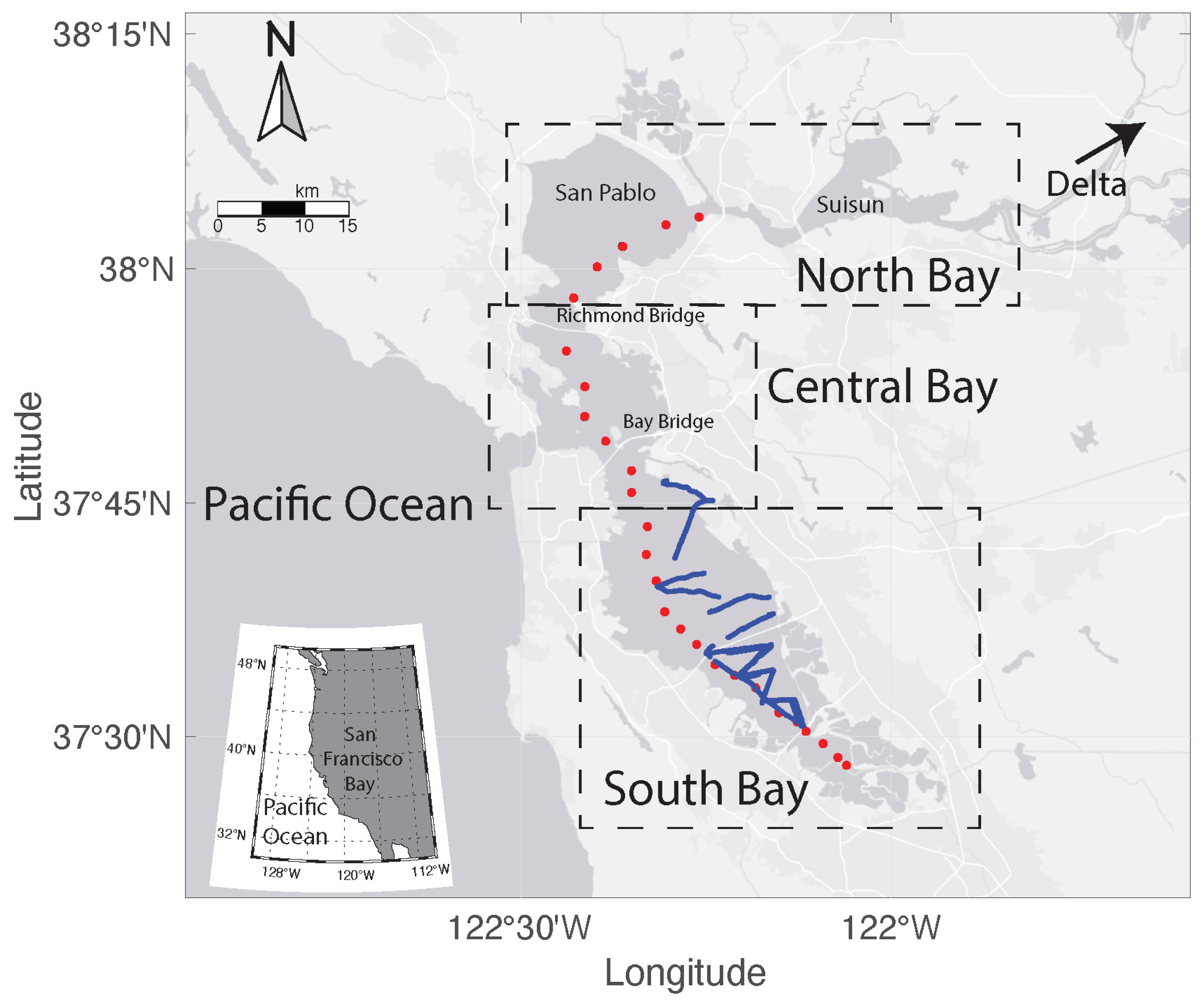
2.1. Study Area
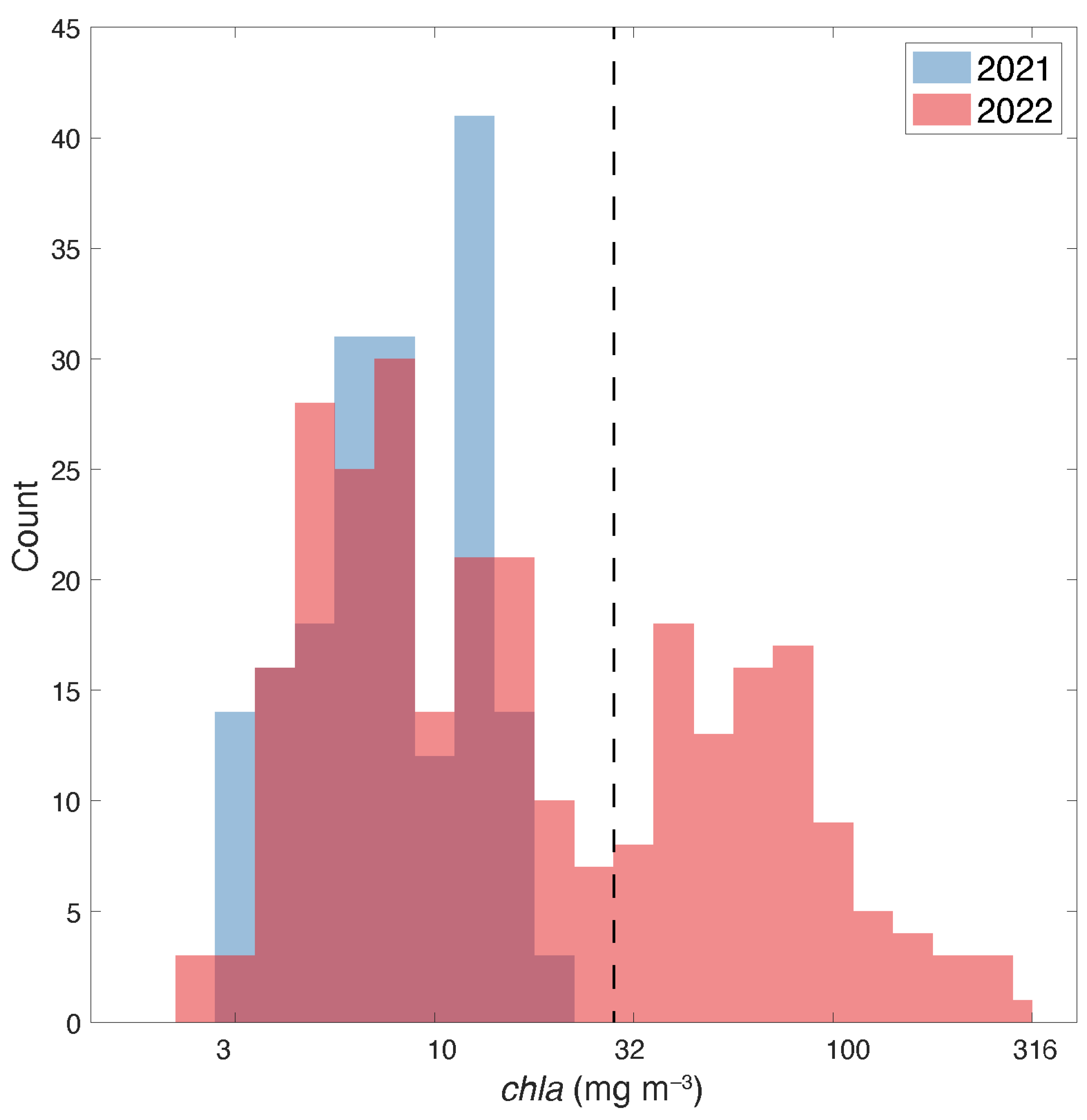
2.2. Data Overview
2.3. Model Tuning Data
2.4. Model Validation Data
2.5. Chla Algorithms
2.6. Algorithm Performance
3. Results
3.1. Field chla and Spectral Absorption Data
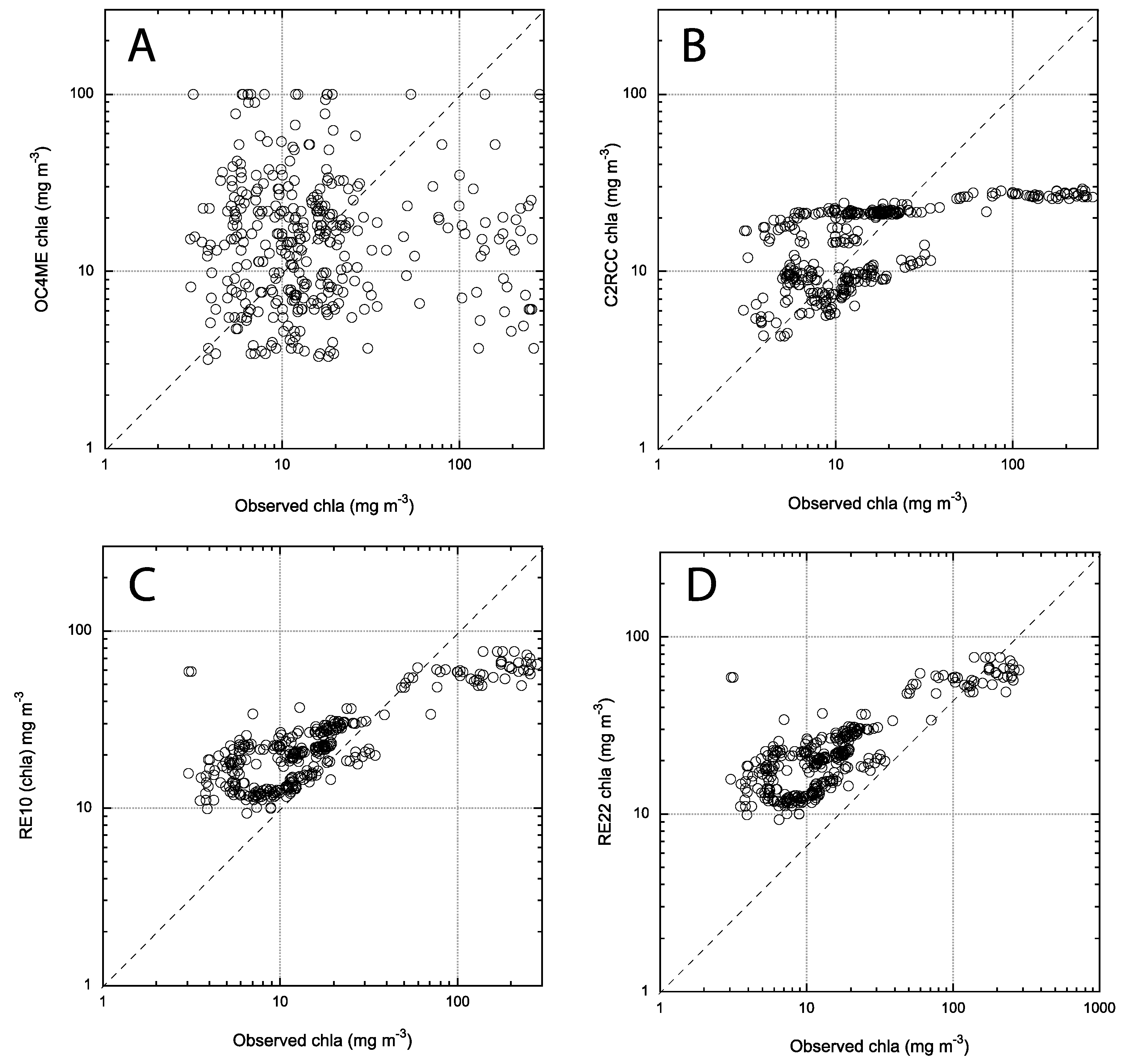
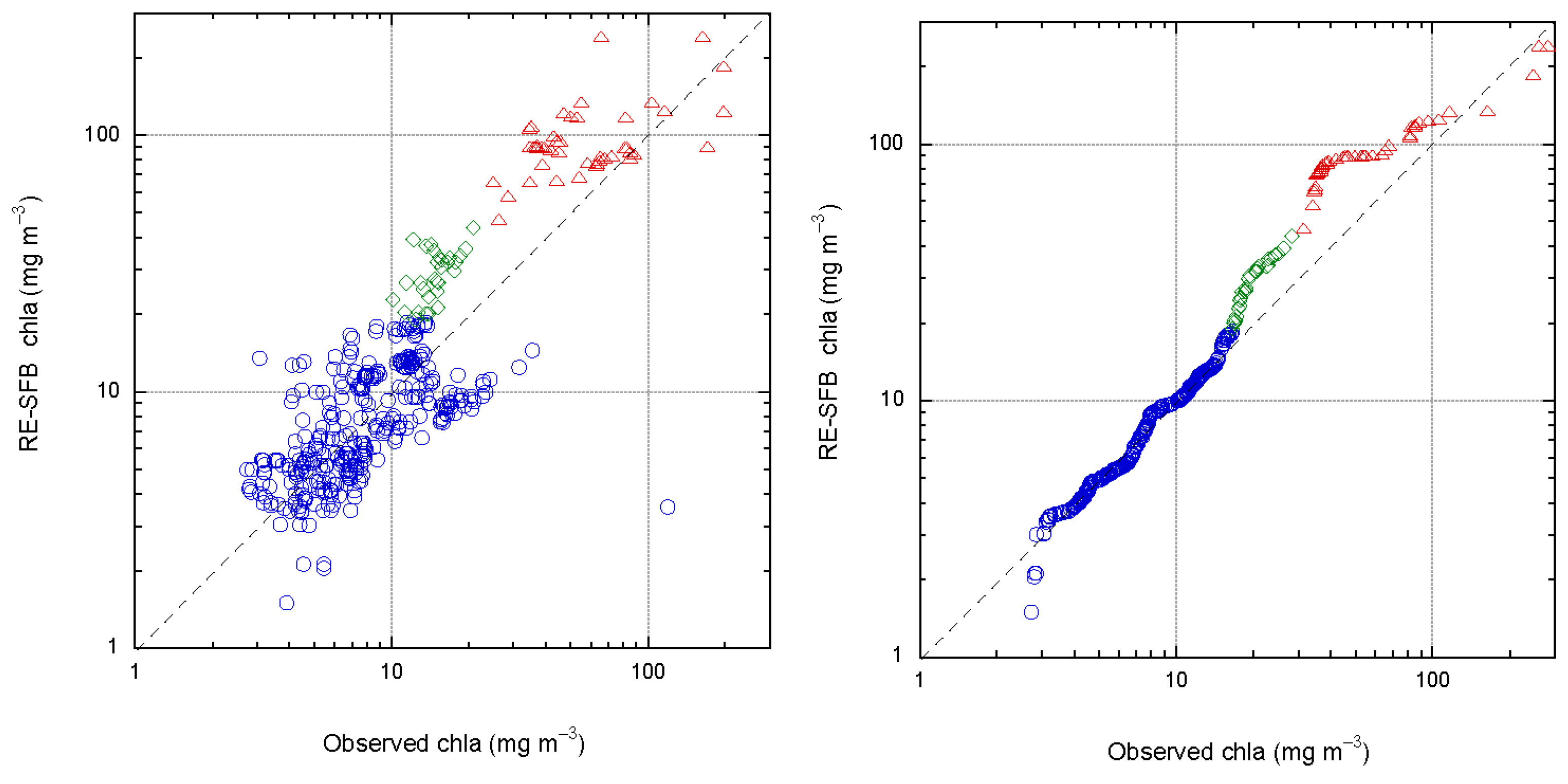
3.2. Matchup between Field chla and OC4Me, RE10, RE22, RE-SFB
3.3. Error Metrics for the Algorithms
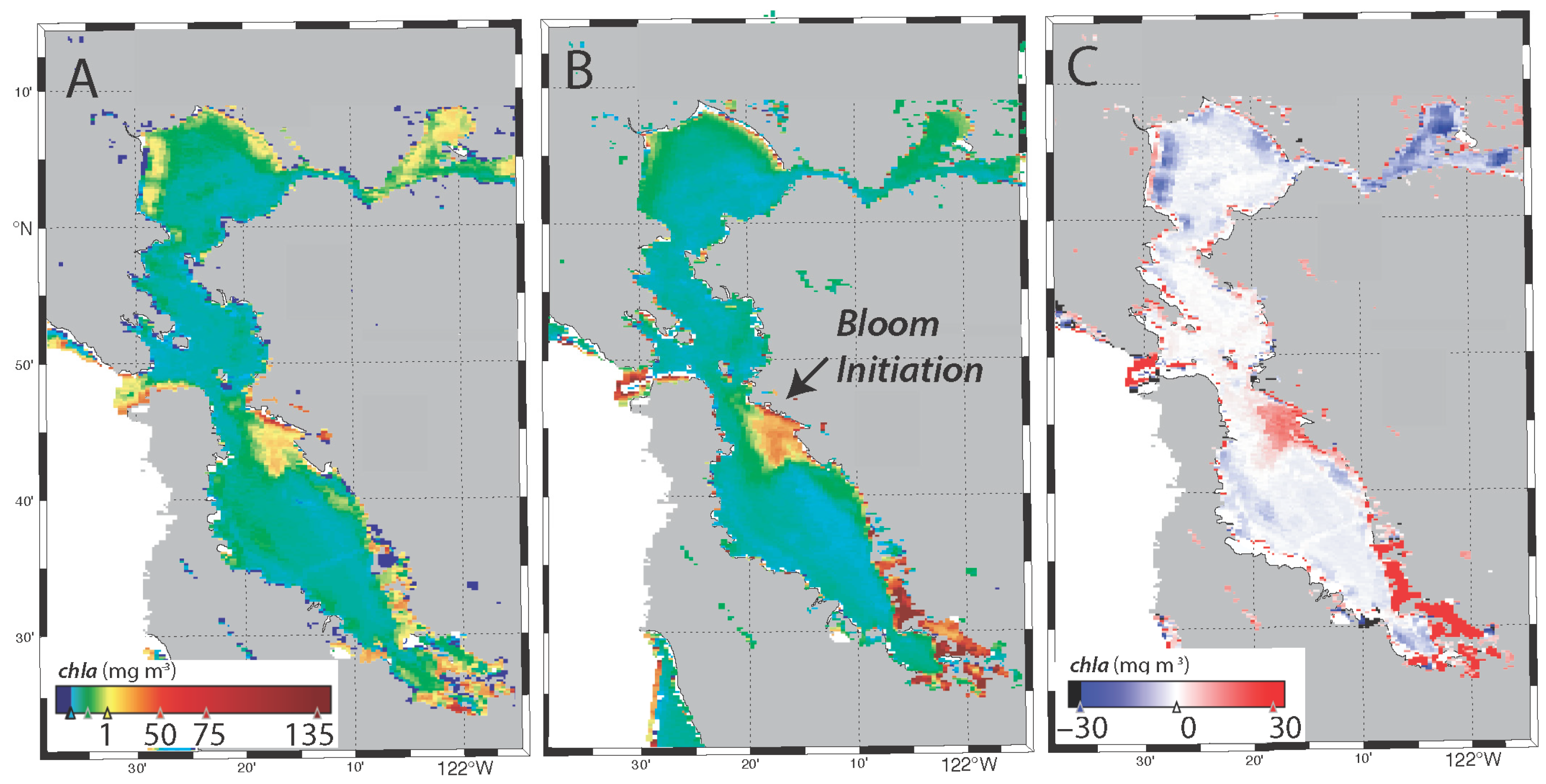
3.4. Spatial Distribution of the Bloom
4. Discussion
5. Conclusions
Supplementary Materials
Author Contributions
Funding
Data Availability Statement
Acknowledgments
Conflicts of Interest
References
- Conomos, T.J.; Smith, R.E.; Gartner, J.W. Environmental Setting of San Francisco Bay. Hydrobiologia 1985, 129, 1–12. [Google Scholar] [CrossRef]
- Sutula, M.; Kudela, R.; Hagy, J.D.; Harding, L.W.; Senn, D.; Cloern, J.E.; Bricker, S.; Berg, G.M.; Beck, M. Novel Analyses of Long-Term Data Provide a Scientific Basis for Chlorophyll-a Thresholds in San Francisco Bay. Estuar. Coast. Shelf Sci. 2017, 197, 107–118. [Google Scholar] [CrossRef] [PubMed]
- Kudela, R.; Howard, M.; Monismith, S.; Paerl, H. Status, Trends, and Drivers of Harmful Algal Blooms Along the Freshwater-to-Marine Gradient in the San Francisco Bay–Delta System. San Franc. Estuary Watershed Sci. 2023, 20, 6. [Google Scholar] [CrossRef]
- Boesch, D.F.; Brinsfield, R.B.; Magnien, R.E. Chesapeake Bay Eutrophication: Scientific Understanding, Ecosystem Restoration, and Challenges for Agriculture. J. Environ. Qual. 2001, 30, 303–320. [Google Scholar] [CrossRef]
- Bricker, S.B.; Longstaff, B.; Dennison, W.; Jones, A.; Boicourt, K.; Wicks, C.; Woerner, J. Effects of Nutrient Enrichment in the Nation’s Estuaries: A Decade of Change. Harmful Algae 2008, 8, 21–32. [Google Scholar] [CrossRef]
- Nixon, S.W. Coastal Marine Eutrophication: A Definition, Social Causes, and Future Concerns. Ophelia 1995, 41, 199–219. [Google Scholar] [CrossRef]
- Diaz, R.J.; Rosenberg, R. Spreading Dead Zones and Consequences for Marine Ecosystems. Science 2008, 321, 926–929. [Google Scholar] [CrossRef]
- Heisler, J.; Glibert, P.M.; Burkholder, J.M.; Anderson, D.M.; Cochlan, W.; Dennison, W.C.; Dortch, Q.; Gobler, C.J.; Heil, C.A.; Humphries, E.; et al. Eutrophication and Harmful Algal Blooms: A Scientific Consensus. Harmful Algae 2008, 8, 3–13. [Google Scholar] [CrossRef]
- Cloern, J. Does the Benthos Control Phytoplankton Biomass in South San Francisco Bay? Mar. Ecol. Prog. Ser. 1982, 9, 191–202. [Google Scholar] [CrossRef]
- Cloern, J.E. Phytoplankton Bloom Dynamics in Coastal Ecosystems: A Review with Some General Lessons from Sustained Investigation of San Francisco Bay, California. Rev. Geophys. 1996, 34, 127–168. [Google Scholar] [CrossRef]
- Jessup, D.A.; Miller, M.A.; Ryan, J.P.; Nevins, H.M.; Kerkering, H.A.; Mekebri, A.; Crane, D.B.; Johnson, T.A.; Kudela, R.M. Mass Stranding of Marine Birds Caused by a Surfactant-Producing Red Tide. PLoS ONE 2009, 4, e4550. [Google Scholar] [CrossRef]
- Cloern, J.E.; Schraga, T.S.; Lopez, C.B.; Knowles, N.; Grover Labiosa, R.; Dugdale, R. Climate Anomalies Generate an Exceptional Dinoflagellate Bloom in San Francisco Bay. Geophys. Res. Lett. 2005, 32, L14608. [Google Scholar] [CrossRef]
- Flores-Leñero, A.; Vargas-Torres, V.; Paredes-Mella, J.; Norambuena, L.; Fuenzalida, G.; Lee-Chang, K.; Mardones, J.I. Heterosigma Akashiwo in Patagonian Fjords: Genetics, Growth, Pigment Signature and Role of PUFA and ROS in Ichthyotoxicity. Toxins 2022, 14, 577. [Google Scholar] [CrossRef] [PubMed]
- Herndon, J.; Cochlan, W.P. Nitrogen Utilization by the Raphidophyte Heterosigma akashiwo: Growth and Uptake Kinetics in Laboratory Cultures. Harmful Algae 2007, 6, 260–270. [Google Scholar] [CrossRef]
- Herndon, J. Nitrogen Uptake by the Raphidophyte Heterosigma akashiwo: A Laboratory and Field Study; M.A., San Francisco State University: San Francisco, CA, USA, 2003. [Google Scholar]
- Fichot, C.G.; Downing, B.D.; Bergamaschi, B.A.; Windham-Myers, L.; Marvin-DiPasquale, M.; Thompson, D.R.; Gierach, M.M. High-Resolution Remote Sensing of Water Quality in the San Francisco Bay–Delta Estuary. Environ. Sci. Technol. 2016, 50, 573–583. [Google Scholar] [CrossRef]
- Pahlevan, N.; Smith, B.; Binding, C.; Gurlin, D.; Li, L.; Bresciani, M.; Giardino, C. Hyperspectral Retrievals of Phytoplankton Absorption and Chlorophyll-a in Inland and Nearshore Coastal Waters. Remote Sens. Environ. 2021, 253, 112200. [Google Scholar] [CrossRef]
- O’Reilly, J.E.; Werdell, P.J. Chlorophyll Algorithms for Ocean Color Sensors—OC4, OC5 & OC6. Remote Sens. Environ. 2019, 229, 32–47. [Google Scholar] [CrossRef]
- Moses, W.J.; Gitelson, A.A.; Berdnikov, S.; Saprygin, V.; Povazhnyi, V. Operational MERIS-Based NIR-Red Algorithms for Estimating Chlorophyll-a Concentrations in Coastal Waters—The Azov Sea Case Study. Remote Sens. Environ. 2012, 121, 118–124. [Google Scholar] [CrossRef]
- Gilerson, A.A.; Gitelson, A.A.; Zhou, J.; Gurlin, D.; Moses, W.; Ioannou, I.; Ahmed, S.A. Algorithms for Remote Estimation of Chlorophyll-a in Coastal and Inland Waters Using Red and near Infrared Bands. Opt. Express 2010, 18, 24109. [Google Scholar] [CrossRef]
- Wynne, T.T.; Tomlinson, M.C.; Briggs, T.O.; Mishra, S.; Meredith, A.; Vogel, R.L.; Stumpf, R.P. Evaluating the Efficacy of Five Chlorophyll-a Algorithms in Chesapeake Bay (USA) for Operational Monitoring and Assessment. J. Mar. Sci. Eng. 2022, 10, 1104. [Google Scholar] [CrossRef]
- Tran, M.D.; Vantrepotte, V.; Loisel, H.; Oliveira, E.N.; Tran, K.T.; Jorge, D.; Mériaux, X.; Paranhos, R. Band Ratios Combination for Estimating Chlorophyll-a from Sentinel-2 and Sentinel-3 in Coastal Waters. Remote Sens. 2023, 15, 1653. [Google Scholar] [CrossRef]
- Wolny, J.L.; Tomlinson, M.C.; Schollaert Uz, S.; Egerton, T.A.; McKay, J.R.; Meredith, A.; Reece, K.S.; Scott, G.P.; Stumpf, R.P. Current and Future Remote Sensing of Harmful Algal Blooms in the Chesapeake Bay to Support the Shellfish Industry. Front. Mar. Sci. 2020, 7, 337. [Google Scholar] [CrossRef]
- Rodríguez-Benito, C.V.; Navarro, G.; Caballero, I. Using Copernicus Sentinel-2 and Sentinel-3 Data to Monitor Harmful Algal Blooms in Southern Chile during the COVID-19 Lockdown. Mar. Pollut. Bull. 2020, 161, 111722. [Google Scholar] [CrossRef]
- Jordan, C.; Cusack, C.; Tomlinson, M.C.; Meredith, A.; McGeady, R.; Salas, R.; Gregory, C.; Croot, P.L. Using the Red Band Difference Algorithm to Detect and Monitor a Karenia Spp. Bloom Off the South Coast of Ireland, June 2019. Front. Mar. Sci. 2021, 8, 638889. [Google Scholar] [CrossRef]
- Kahru, M.; Anderson, C.; Barton, A.D.; Carter, M.L.; Catlett, D.; Send, U.; Sosik, H.M.; Weiss, E.L.; Mitchell, B.G. Satellite Detection of Dinoflagellate Blooms off California by UV Reflectance Ratios. Elem. Sci. Anthr. 2021, 9, 00157. [Google Scholar] [CrossRef]
- Windle, A.E.; Evers-King, H.; Loveday, B.R.; Ondrusek, M.; Silsbe, G.M. Evaluating Atmospheric Correction Algorithms Applied to OLCI Sentinel-3 Data of Chesapeake Bay Waters. Remote Sens. 2022, 14, 1881. [Google Scholar] [CrossRef]
- Brockmann, C.; Doerffer, R.; Peters, M.; Stelzer, K.; Embacher, S.; Ruescas, A. Evolution of the C2RCC Neural Network for Sentinel 2 and 3 for the Retrieval of Ocean Color Products in Normal and Extreme Optically Complex Waters. In Proceedings of the Living Planet Symposium 2016, Prague, Czech Republic, 9 May 2016; European Space Agency Special Publication: Prague, Czech Republic, 2016; Volume ESA SP, pp. 1–6. [Google Scholar]
- Stumpf, R.P.; Tyler, M.A. Satellite Detection of Bloom and Pigment Distributions in Estuaries. Remote Sens. Environ. 1988, 24, 385–404. [Google Scholar] [CrossRef]
- Schraga, T.S.; Cloern, J.E. Water Quality Measurements in San Francisco Bay by the U.S. Geological Survey, 1969–2015. Sci. Data 2017, 4, 170098. [Google Scholar] [CrossRef]
- Richardson, E.T.; O’Donnell, K.; Soto Perez, J.; Sturgeon, C.L.; Brinkman, J.; Delascagigas, A.; Nakatsuka, K.; Uebner, M.Q.; Jaegge, A.; Dellwo, P.; et al. Assessing Spatial Variability of Nutrients, Phytoplankton and Related Water-Quality Constituents in the San Francisco Bay, California: 2021–2022 High-Resolution Mapping Surveys; U.S. Geological Survey data release; U.S. Geological Survey: Reston, WV, USA, 2024. [CrossRef]
- Schraga, T.; Nejad, E.S.; Martin, C.A.; Cloern, J.E. USGS Measurements of Water Quality in San Francisco Bay (CA), 2016–2021 (Ver. 4.0, March 2023); U.S. Geological Survey Data Release; U.S. Geological Survey: Reston, WV, USA, 2018. [CrossRef]
- Morel, A.; Huot, Y.; Gentili, B.; Werdell, P.J.; Hooker, S.B.; Franz, B.A. Examining the Consistency of Products Derived from Various Ocean Color Sensors in Open Ocean (Case 1) Waters in the Perspective of a Multi-Sensor Approach. Remote Sens. Environ. 2007, 111, 69–88. [Google Scholar] [CrossRef]
- Stramski, D.; Reynolds, R.A.; Kaczmarek, S.; Uitz, J.; Zheng, G. Correction of Pathlength Amplification in the Filter-Pad Technique for Measurements of Particulate Absorption Coefficient in the Visible Spectral Region. Appl. Opt. 2015, 54, 6763. [Google Scholar] [CrossRef]
- Seegers, B.N.; Stumpf, R.P.; Schaeffer, B.A.; Loftin, K.A.; Werdell, P.J. Performance Metrics for the Assessment of Satellite Data Products: An Ocean Color Case Study. Opt. Express 2018, 26, 7404. [Google Scholar] [CrossRef] [PubMed]
- Le, C.; Hu, C.; English, D.; Cannizzaro, J.; Kovach, C. Climate-Driven Chlorophyll-a Changes in a Turbid Estuary: Observations from Satellites and Implications for Management. Remote Sens. Environ. 2013, 130, 11–24. [Google Scholar] [CrossRef]
- Chen, J.; Pan, D.; Liu, M.; Mao, Z.; Zhu, Q.; Chen, N.; Zhang, X.; Tao, B. Relationships between Long-Term Trend of Satellite-Derived Chlorophyll-a and Hypoxia Off the Changjiang Estuary. Estuaries Coasts 2017, 40, 1055–1065. [Google Scholar] [CrossRef]
- Keith, D.J. Satellite Remote Sensing of Chlorophyll a in Support of Nutrient Management in the Neuse and Tar–Pamlico River (North Carolina) Estuaries. Remote Sens. Environ. 2014, 153, 61–78. [Google Scholar] [CrossRef]
- Conmy, R.N.; Schaeffer, B.A.; Schubauer-Berigan, J.; Aukamp, J.; Duffy, A.; Lehrter, J.C.; Greene, R.M. Characterizing Light Attenuation within Northwest Florida Estuaries: Implications for RESTORE Act Water Quality Monitoring. Mar. Pollut. Bull. 2017, 114, 995–1006. [Google Scholar] [CrossRef]
- Kim, Y.; Yoo, S.; Son, Y.B. Optical Discrimination of Harmful Cochlodinium Polykrikoides Blooms in Korean Coastal Waters. Opt. Express 2016, 24, A1471. [Google Scholar] [CrossRef] [PubMed]
- Mograne, M.; Jamet, C.; Loisel, H.; Vantrepotte, V.; Mériaux, X.; Cauvin, A. Evaluation of Five Atmospheric Correction Algorithms over French Optically-Complex Waters for the Sentinel-3A OLCI Ocean Color Sensor. Remote Sens. 2019, 11, 668. [Google Scholar] [CrossRef]
- Taylor, N.C.; Kudela, R.M. Spatial Variability of Suspended Sediments in San Francisco Bay, California. Remote Sens. 2021, 13, 4625. [Google Scholar] [CrossRef]
- Franz, B.A.; Bailey, S.W.; Kuring, N.; Werdell, P.J. Ocean Color Measurements with the Operational Land Imager on Landsat-8: Implementation and Evaluation in SeaDAS. J. Appl. Remote Sens. 2015, 9, 096070. [Google Scholar] [CrossRef]
- Bramich, J.; Bolch, C.J.S.; Fischer, A. Improved Red-Edge Chlorophyll-a Detection for Sentinel 2. Ecol. Indic. 2021, 120, 106876. [Google Scholar] [CrossRef]
- U.S. Geological Survey. USGS Water Data for the Nation: U.S. Geological Survey National. Water Information System Database. 2024. Available online: https://waterdata.usgs.gov/nwis (accessed on 8 March 2024).


| Algorithm | n * | R2 | Slope | RMSE | MAE | MBIAS | MedAE | MedBIAS |
|---|---|---|---|---|---|---|---|---|
| OC4Me | 415 | 0.615 | 0.654 | 0.370 | 2.235 | 1.707 | 2.127 | 1.840 |
| C2RCC | 351 | −0.003 | −0.012 | 0.544 | 3.314 | 0.870 | 3.421 | 1.266 |
| RE10 | 426 | 0.319 | 1.786 | 0.425 | 2.316 | 1.843 | 2.301 | 2.084 |
| RE22 | 426 | 0.380 | 1.418 | 0.381 | 2.136 | 1.488 | 2.074 | 1.799 |
| RE-SFB | 425 | 0.891 | 0.865 | 0.203 | 1.469 | 0.964 | 1.398 | 0.991 |
| Algorithm | n * | R2 | Slope | RMSE | MAE | MBIAS | MedAE | MedBIAS |
|---|---|---|---|---|---|---|---|---|
| OC4Me | 354 | 0.019 | 0.171 | 0.370 | 1.934 | 1.450 | 1.760 | 1.760 |
| C2RCC | 257 | 0.001 | 0.082 | 0.544 | 2.815 | 1.026 | 2.534 | 2.534 |
| RE10 | 359 | 0.350 | 0.385 | 0.425 | 2.310 | 1.998 | 2.408 | 2.408 |
| RE22 | 359 | 0.477 | 0.390 | 0.381 | 2.111 | 1.636 | 2.106 | 2.106 |
| RE-SFB | 359 | 0.489 | 0.841 | 0.197 | 1.460 | 0.963 | 1.395 | 0.927 |
| Algorithm | n * | R2 | Slope | RMSE | MAE | MBIAS | MedAE | MedBIAS |
|---|---|---|---|---|---|---|---|---|
| OC4Me | 61 | 0.001 | 0.026 | 0.984 | 7.324 | 0.155 | 6.470 | 0.155 |
| C2RCC | 94 | 0.568 | 0.077 | 0.666 | 3.972 | 0.297 | 4.702 | 0.213 |
| RE10 | 67 | 0.625 | 0.067 | 0.549 | 3.138 | 0.432 | 3.323 | 0.308 |
| RE22 | 67 | 0.771 | 0.335 | 0.390 | 2.172 | 0.569 | 2.350 | 0.458 |
| RE-SFB | 66 | 0.801 | 0.588 | 0.233 | 1.548 | 1.178 | 1.412 | 1.012 |
Disclaimer/Publisher’s Note: The statements, opinions and data contained in all publications are solely those of the individual author(s) and contributor(s) and not of MDPI and/or the editor(s). MDPI and/or the editor(s) disclaim responsibility for any injury to people or property resulting from any ideas, methods, instructions or products referred to in the content. |
© 2024 by the authors. Licensee MDPI, Basel, Switzerland. This article is an open access article distributed under the terms and conditions of the Creative Commons Attribution (CC BY) license (https://creativecommons.org/licenses/by/4.0/).
Share and Cite
Kudela, R.M.; Senn, D.B.; Richardson, E.T.; Bouma-Gregson, K.; Bergamaschi, B.A.; Sim, L. Evaluation and Refinement of Chlorophyll-a Algorithms for High-Biomass Blooms in San Francisco Bay (USA). Remote Sens. 2024, 16, 1103. https://doi.org/10.3390/rs16061103
Kudela RM, Senn DB, Richardson ET, Bouma-Gregson K, Bergamaschi BA, Sim L. Evaluation and Refinement of Chlorophyll-a Algorithms for High-Biomass Blooms in San Francisco Bay (USA). Remote Sensing. 2024; 16(6):1103. https://doi.org/10.3390/rs16061103
Chicago/Turabian StyleKudela, Raphael M., David B. Senn, Emily T. Richardson, Keith Bouma-Gregson, Brian A. Bergamaschi, and Lawrence Sim. 2024. "Evaluation and Refinement of Chlorophyll-a Algorithms for High-Biomass Blooms in San Francisco Bay (USA)" Remote Sensing 16, no. 6: 1103. https://doi.org/10.3390/rs16061103