
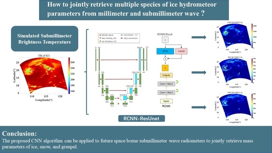
Joint Retrieval of Multiple Species of Ice Hydrometeor Parameters from Millimeter and Submillimeter Wave Brightness Temperature Based on Convolutional Neural Networks


Abstract
:
1. Introduction
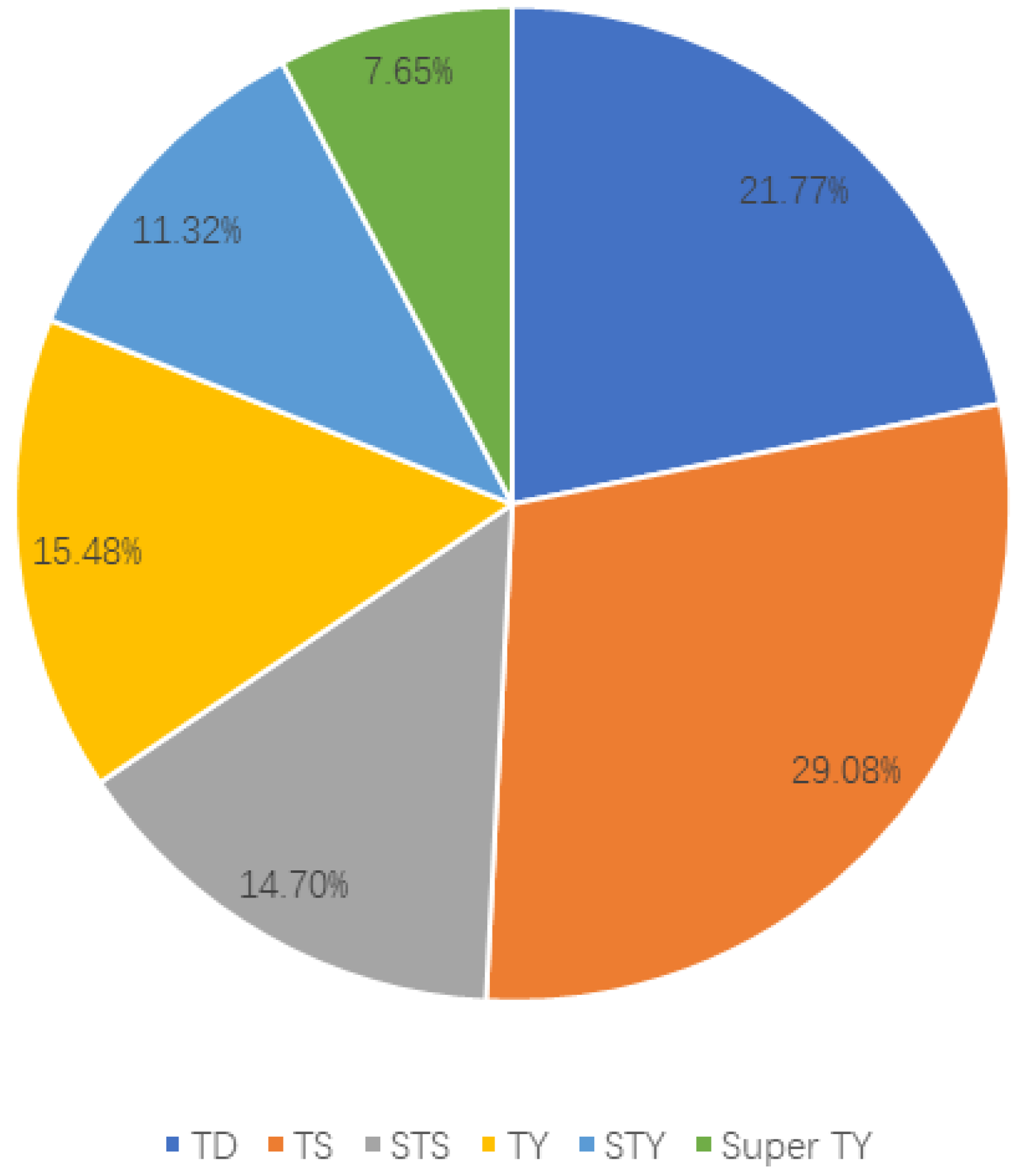
2. Dataset
2.1. Simulated Brightness Temperature Verification
2.2. Construction of the Ice Cloud Dataset
2.3. Constructing the TB Dataset
3. Algorithm Introduction
3.1. Unet
3.2. RCNN–ResUnet
4. Ice Cloud Parameter Retrieval Experiments
4.1. Multiple Species of Ice Hydrometeors Retrieval from the Simulated ICI Brightness Temperature
4.1.1. Joint Retrieval of Water Paths of Multiple Species of Ice Hydrometeors
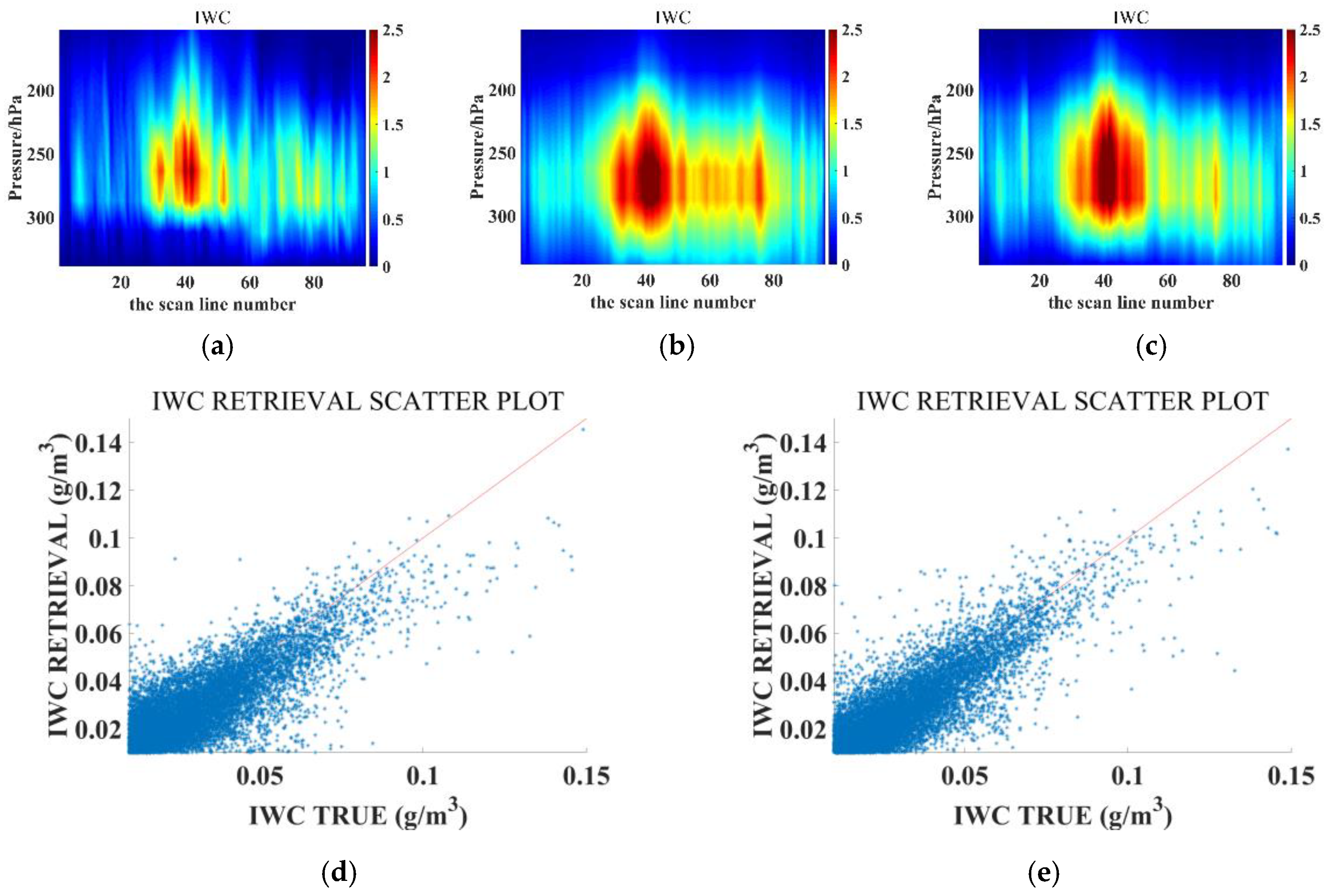
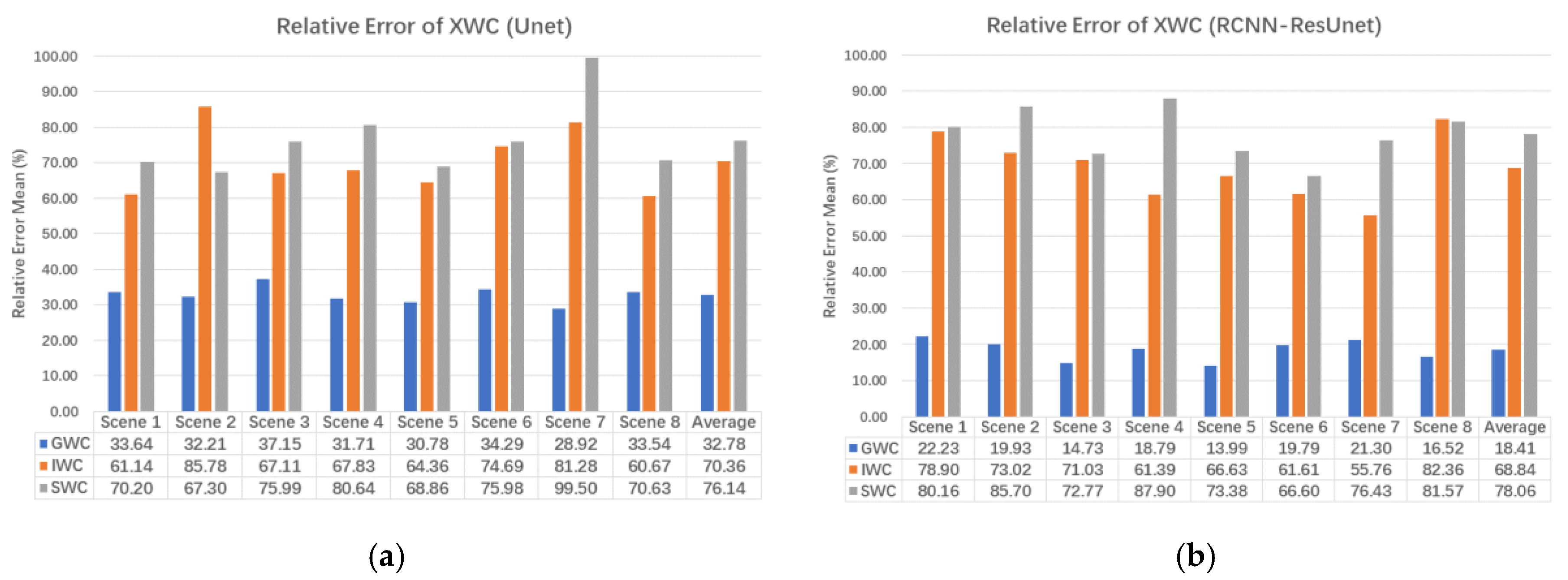
4.1.2. Joint Retrieval of Multiple Species of Ice Water Contents
4.2. Graupel Parameter Retrieval from the Actual ATMS Brightness Temperature
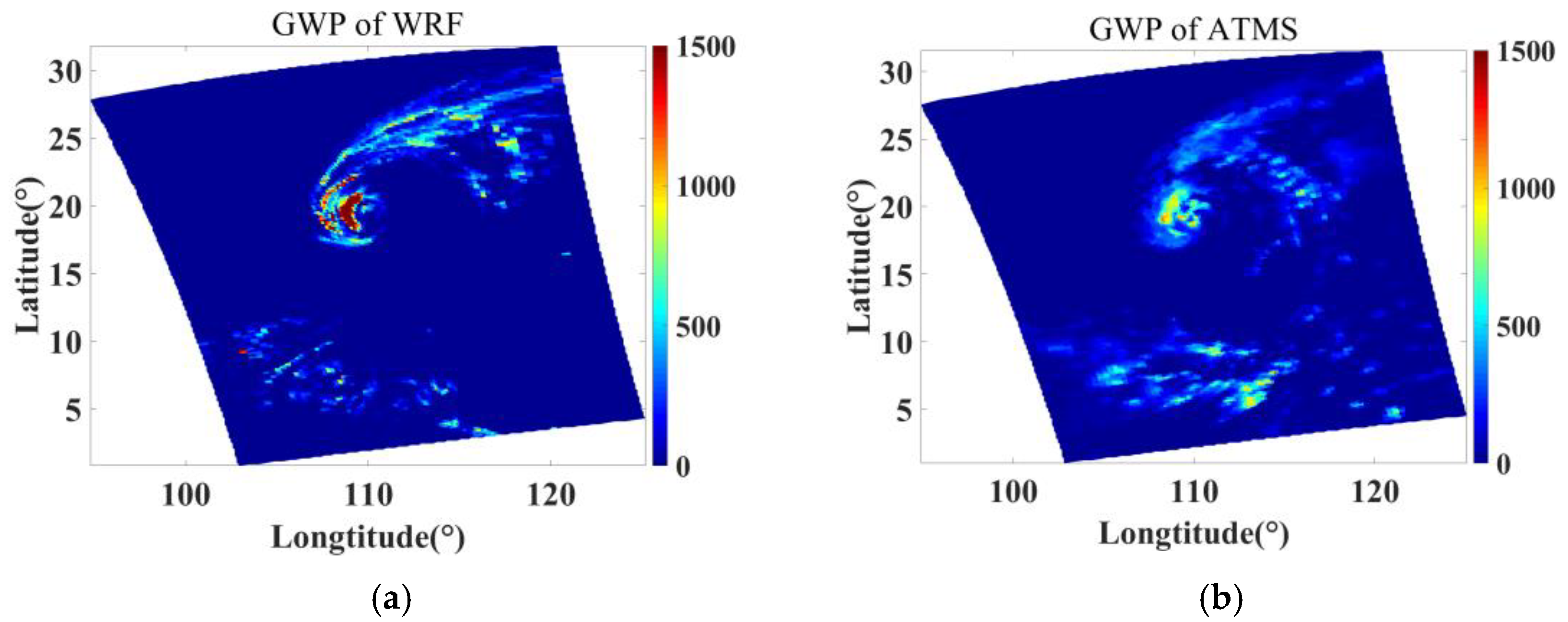
4.2.1. Retrieval of the Graupel Water Path (GWP)
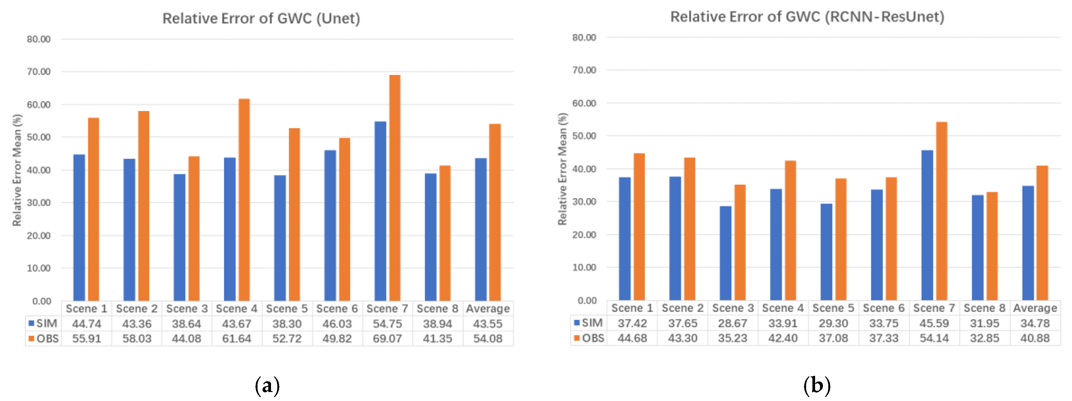
4.2.2. Retrieval of Graupel Water Content (GWC)
4.2.3. The Sensitivity Experiments for the Retrieval of Graupel Parameters
4.3. Comparison of the Retrieval Performance of Unet and RCNN–ResUnet
5. Conclusions and Discussion
Author Contributions
Funding
Data Availability Statement
Acknowledgments
Conflicts of Interest
References
- Wang, H.; Duan, C.; Lv, R.; Lei, H.; Zhu, Z.; Chen, G. Development and Problems of Spaceborne Terahertz Ice Cloud Detection Technology. J. Terahertz Sci. Electron. Inf. Technol. 2017, 5, 722–727. [Google Scholar]
- Zhang, X.; Hu, W.; Liu, R.; Si, W.; Li, Y.; Liu, Y.; Ligthart, L.P. Design of 874 GHz Ice Cloud Detection Instrument Based on Cubesat Platform. Aerosp. Shanghai 2018, 35, 144–150. [Google Scholar]
- Buehler, S.A.; Jiménez, C.; Evans, K.F.; Eriksson, P.; Rydberg, B.; Heymsfield, A.J.; Stubenrauch, C.J.; Lohmann, U.; Emde, C.; John, V.O.; et al. A concept for a satellite mission to measure cloud ice water path, ice particle size, and cloud altitude. Q. J. R. Meteorol. Soc. J. Atmos. Sci. Appl. Meteorol. Phys. Oceanogr. 2007, 133, 109–128. [Google Scholar] [CrossRef]
- Liou, K.-N. Influence of cirrus clouds on weather and climate processes: A global perspective. Mon. Weather. Rev. 1986, 114, 1167–1199. [Google Scholar] [CrossRef]
- Njoku, E. Passive microwave remote sensing of the earth from space—A review. Proc. IEEE 1982, 70, 728–750. [Google Scholar] [CrossRef]
- Gustavsson, K.; Sheikh, M.Z.; Naso, A.; Pumir, A.; Mehlig, B. Effect of particle inertia on the alignment of small ice crystals in turbulent clouds. J. Atmos. Sci. 2021, 78, 2573–2587. [Google Scholar] [CrossRef]
- Skolnik, M.I. Millimeter and submillimeter wave applications. In Proceedings of the Symposium on Submillimeter Waves, Polytechnic Press of Poly, New York, NY, USA, 31 March–2 April 1970; Institute of Brooklyn: New York, NY, USA, 1970. [Google Scholar]
- Kidder, S.Q.; Goldberg, M.D.; Zehr, R.M.; DeMaria, M.; Purdom, J.F.W.; Velden, C.S.; Grody, N.C.; Kusselson, S.J. Satellite analysis of tropical cyclones using the Advanced Microwave Sounding Unit (AMSU). Bull. Am. Meteorol. Soc. 2000, 81, 1241–1259. [Google Scholar] [CrossRef]
- Bonsignori, R. The Microwave Humidity Sounder (MHS): In-orbit performance assessment. In Proceedings of the Sensors, Systems, and Next-Generation Satellites XI, Florence, Italy, 17–20 September 2007; p. 67440A. [Google Scholar]
- Weng, F.; Zou, X.; Wang, X.; Yang, S.; Goldberg, M.D. Introduction to Suomi national polar-orbiting partnership advanced technology microwave sounder for numerical weather prediction and tropical cyclone applications. J. Geophys. Res. Atmos. 2012, 117, D19112. [Google Scholar] [CrossRef]
- Chen, K.; English, S.; Bormann, N.; Zhu, J. Assessment of FY-3A and FY-3B MWHS observations. Weather Forecast. 2015, 30, 1280–1290. [Google Scholar] [CrossRef]
- Zou, X.; Wang, X.; Weng, F.; Li, G. Assessments of Chinese Fengyun Microwave Temperature Sounder (MWTS) measurements for weather and climate applications. J. Atmos. Ocean. Technol. 2011, 28, 1206–1227. [Google Scholar] [CrossRef]
- Kangas, V.; D’Addio, S.; Klein, U.; Loiselet, M.; Mason, G.; Orlhac, J.C.; Gonzalez, R.; Bergada, M.; Brandt, M.; Thomas, B. Ice cloud imager instrument for MetOp Second Generation. In Proceedings of the 2014 13th Specialist Meeting on Microwave Radiometry and Remote Sensing of the Environment (MicroRad), Pasadena, CA, USA, 24–27 March 2014. [Google Scholar]
- Schlussel, P.; Kayal, G. Introduction to the next generation EUMETSAT polar system (EPS-SG) observation missions. In Proceedings of the Conference on Sensors, Systems, and Next-Generation Satellites XX, Warsaw, Poland, 11–14 September 2017. [Google Scholar]
- Evans, K.F.; Graeme, L.S. Microwave radiative transfer through clouds composed of realistically shaped ice crystals. Part I. Single scattering properties. J. Atmos. Sci. 1995, 52, 2041–2057. [Google Scholar]
- Evans, K.F.; Stephens, G.L. Microweve radiative transfer through clouds composed of realistically shaped ice crystals. Part II. Remote sensing of ice clouds. J. Atmos. Sci. 1995, 52, 2058–2072. [Google Scholar] [CrossRef]
- Evans, K.F.; Wang, J.R.; O’C Starr, D.; Heymsfield, G.; Li, L.; Tian, L.; Lawson, R.P.; Heymsfield, A.J.; Bansemer, A. Ice hydrometeor profile retrieval algorithm for high-frequency microwave radiometers: Application to the CoSSIR instrument during TC4. Atmos. Meas. Tech. 2012, 5, 2277–2306. [Google Scholar] [CrossRef]
- Buehler, S.A.; Eriksson, P.; Kuhn, T.; von Engeln, A.; Verdes, C. ARTS, the atmospheric radiative transfer simulator. J. Quant. Spectrosc. Radiat. Transf. 2005, 91, 65–93. [Google Scholar] [CrossRef]
- Jiménez, C.; Buehler, S.A.; Rydberg, B.; Eriksson, P.; Evans, K.F. Performance simulations for a submillimetre-wave satellite instrument to measure cloud ice. Q. J. R. Meteorol. Soc. J. Atmos. Sci. Appl. Meteorol. Phys. Oceanogr. 2007, 133, 129–149. [Google Scholar] [CrossRef]
- Weng, F.; Grody, N.C. Retrieval of ice cloud parameters USING a microwave imaging radiometer. J. Atmos. Sci. 2000, 57, 1069–1081. [Google Scholar] [CrossRef]
- Dong, P.; Liu, L.; Li, S.; Husi, L.; Hu, S.; Bu, L. A novel Ice Cloud Retrieval Algorithm for Sub-Millimeter Wave Radiometers: Simulations and Application to an Airborne Experiment. IEEE Trans. Geosci. Remote Sens. 2023, 61, 2001609. [Google Scholar] [CrossRef]
- Li, M.; Letu, H.; Ishimoto, H.; Li, S.; Liu, L.; Nakajima, T.Y.; Ji, D.; Shang, H.; Shi, C. Retrieval of terahertz ice cloud properties from airborne measurements based on the irregularly shaped Voronoi ice scattering models. Atmos. Meas. Tech. 2023, 16, 331–353. [Google Scholar] [CrossRef]
- Eriksson, P.; Rydberg, B.; Mattioli, V.; Thoss, A.; Accadia, C.; Klein, U.; Buehler, S.A. Towards an operational Ice Cloud Imager (ICI) retrieval product. Atmos. Meas. Tech. 2020, 13, 53–71. [Google Scholar] [CrossRef]
- Chen, K.; Zhang, L.; Zhang, Y.; Dong, S.; Liu, Y.; Wu, Q.; Shang, J. Study on Terahertz Ice Cloud Detection Inversion Algorithm Based on Neural Network. J. Remote Sens. 2022, 26, 2043–2059. [Google Scholar]
- Powers, J.G.; Klemp, J.B.; Skamarock, W.C.; Davis, C.A.; Dudhia, J.; Gill, D.O.; Coen, J.L.; Gochis, D.J.; Ahmadov, R.; Peckham, S.E.; et al. The weather research and forecasting model: Overview, system efforts, and future directions. Bull. Am. Meteorol. Soc. 2017, 98, 1717–1737. [Google Scholar] [CrossRef]
- Bauer, P.; Moreau, E.; Chevallier, F.; O’keeffe, U. Multiple-scattering microwave radiative transfer for data assimilation applications. Q. J. R. Meteorol. Soc. J. Atmos. Sci. Appl. Meteorol. Phys. Oceanogr. 2006, 132, 1259–1281. [Google Scholar] [CrossRef]
- Voronovich, A.; Gasiewski, A.; Weber, B. A fast multistream scattering-based Jacobian for microwave radiance assimilation. IEEE Trans. Geosci. Remote Sens. 2004, 42, 1749–1761. [Google Scholar] [CrossRef]
- O’Shea, K.; Nash, R. An introduction to convolutional neural networks. arXiv 2015, arXiv:1511.08458. [Google Scholar]
- Guo, Y.; Chen, E.; Guo, Y.; Li, Z.; Li, C.; Xu, K. Deep highway unit network for land cover type classification with GF-3 SAR imagery. In Proceedings of the 2017 SAR in Big Data Era: Models, Methods and Applications (BIGSARDATA), Beijing, China, 13–14 November 2017; pp. 1–6. [Google Scholar]
- Pai, M.M.; Mehrotra, V.; Aiyar, S.; Verma, U.; Pai, R.M. Automatic segmentation of river and land in sar images: A deep learning approach. In Proceedings of the 2019 IEEE Second International Conference on Artificial Intelligence and Knowledge Engineering (AIKE), Sardinia, Italy, 3–5 June 2019. [Google Scholar]
- Yao, Q.; Hu, X.; Lei, H. Multiscale convolutional neural networks for geospatial object detection in VHR satellite images. IEEE Geosci. Remote Sens. Lett. 2020, 18, 23–27. [Google Scholar] [CrossRef]
- Wang, L.; Scott, K.A.; Clausi, D.A. Sea ice concentration estimation during freeze-up from SAR imagery using a convolutional neural network. Remote Sens. 2017, 9, 408. [Google Scholar] [CrossRef]
- Cooke, C.L.V.; Scott, K.A. Estimating sea ice concentration From SAR: Training convolutional neural networks with passive microwave data. IEEE Trans. Geosci. Remote Sens. 2019, 57, 4735–4747. [Google Scholar] [CrossRef]
- Tan, J.; NourEldeen, N.; Mao, K.; Shi, J.; Li, Z.; Xu, T.; Yuan, Z. Deep learning convolutional neural network for the retrieval of land surface temperature from AMSR2 DATA in China. Sensors 2019, 19, 2987. [Google Scholar] [CrossRef] [PubMed]
- Tan, J.C. Research on Inversion Methods of Key Parameters for Water Conservation Based on Remote Sensing Data. Master’s Thesis, Chinese Academy of Agricultural Sciences, Beijing, China, 2019. [Google Scholar]
- Hersbach, H.; Bell, B.; Berrisford, P.; Hirahara, S.; Horányi, A.; Muñoz-Sabater, J.; Nicolas, J.; Peubey, C.; Radu, R.; Schepers, D.; et al. The ERA5 global reanalysis. Q. J. R. Meteorol. Soc. 2020, 146, 1999–2049. [Google Scholar] [CrossRef]
- Zhou, L.; Divakarla, M.; Liu, X. An overview of the Joint Polar Satellite System (JPSS) science data product calibration and validation. Remote Sens. 2016, 8, 139. [Google Scholar] [CrossRef]
- Chen, K.; Dong, S.; Li, Y.; Xu, H.; Xie, Z.; Jiang, L.; Li, E.; Wu, Q.; Shang, J. Study on Terahertz Ice Cloud Radiation Scattering Characteristics and Detection Parameter Design. J. Remote Sens. 2022, 26, 2204–2218. [Google Scholar]
- Lang, S.E.; Tao, W.K.; Zeng, X.; Li, Y. Reducing the biases in simulated radar reflectivities from a bulk microphysics scheme: Tropical convective systems. J. Atmos. Sci. 2011, 68, 2306–2320. [Google Scholar] [CrossRef]
- Heymsfield, A.J.; Iaquinta, J. Cirrus crystal terminal velocities. J. Atmos. Sci. 2000, 57, 916–938. [Google Scholar] [CrossRef]
- Ronneberger, O.; Fischer, P.; Brox, T. U-net: Convolutional networks for biomedical image segmentation. In Proceedings of the Medical Image Computing and Computer-Assisted Intervention–MICCAI 2015: 18th International Conference, Munich, Germany, 5–9 October 2015; Proceedings, Part III 18. Springer International Publishing: Munich, Germany, 2015. [Google Scholar]
- Wan, C.; Wu, J.; Li, H.; Yan, Z.; Wang, C.; Jiang, Q.; Cao, G.; Xu, Y.; Yang, W. Optimized-Unet: Novel algorithm for parapapillary atrophy segmentation. Front. Neurosci. 2021, 15, 758887. [Google Scholar] [CrossRef] [PubMed]
- Diakogiannis, F.I.; Waldner, F.; Caccetta, P.; Wu, C. ResUNet-a: A deep learning framework for semantic segmentation of remotely sensed data. ISPRS J. Photogramm. Remote Sens. 2020, 162, 94–114. [Google Scholar] [CrossRef]
- Zhou, Z.; Siddiquee, M.M.R.; Tajbakhsh, N.; Liang, J. UNet++: Redesigning skip connections to exploit multiscale features in image segmentation. IEEE Trans. Med. Imaging 2020, 39, 1856–1867. [Google Scholar] [CrossRef]
- Lian, S.; Luo, Z.; Zhong, Z.; Lin, X.; Su, S.; Li, S. Attention guided U-Net for accurate iris segmentation. J. Vis. Commun. Image Represent. 2018, 56, 296–304. [Google Scholar] [CrossRef]
- Liang, M.; Hu, X. Recurrent convolutional neural network for object recognition. In Proceedings of the IEEE Conference on Computer Vision and Pattern Recognition, Boston, MA, USA, 7–12 June 2015. [Google Scholar]
- He, K.; Zhang, X.; Ren, S.; Sun, J. Deep residual learning for image recognition. In Proceedings of the IEEE Conference on Computer Vision and Pattern Recognition, Las Vegas, NV, USA, 27 June–1 July 2016. [Google Scholar]


| Microphysics | Longwave Radiation | Shortwave Radiation | Surface Layer | Land Surface | Planetary Boundary Layer | Cumulus Parameterization |
|---|---|---|---|---|---|---|
| Purdue Lin scheme | RRTM scheme | Dudhia scheme | MM5 similarity | Noah Land Surface Model | Yonsei University scheme | Kain–Fritsch scheme |
| Frequency (GHz) | 165.5 | 183.31 ± 7 | 183.31 ± 4.5 | 183.31 ± 3 | 183.31 ± 1.8 | 183.31 ± 1 | |
|---|---|---|---|---|---|---|---|
| Scene | |||||||
| SARIKA | WRF data | 14.58 | 10.51 | 7.68 | 5.61 | 4.00 | 3.13 |
| ATMS L2 data | 4.37 | 3.22 | 2.93 | 2.55 | 2.18 | 2.21 | |
| NOCK–TEN | WRF data | 11.03 | 8.57 | 6.69 | 5.21 | 3.82 | 2.92 |
| ATMS L2 data | 3.55 | 2.65 | 2.40 | 2.17 | 1.88 | 1.80 | |
| NEOGURI | WRF data | 13.28 | 11.10 | 9.13 | 7.40 | 5.71 | 4.40 |
| ATMS L2 data | 2.90 | 3.24 | 3.12 | 2.92 | 2.57 | 2.48 | |
| FENGSHEN | WRF data | 13.42 | 10.82 | 8.72 | 6.86 | 4.99 | 3.66 |
| ATMS L2 data | 3.35 | 3.43 | 3.18 | 2.83 | 2.35 | 2.18 | |
| FUNG–WONG | WRF data | 12.42 | 9.91 | 8.09 | 6.47 | 4.87 | 3.72 |
| ATMS L2 data | 4.42 | 3.26 | 2.79 | 2.38 | 2.00 | 2.02 | |
| NANGKA | WRF data | 9.75 | 8.16 | 6.76 | 5.56 | 4.45 | 3.64 |
| ATMS L2 data | 2.61 | 2.57 | 2.65 | 2.70 | 2.58 | 2.48 | |
| CHAMPI | WRF data | 8.58 | 7.33 | 6.15 | 5.07 | 3.95 | 3.18 |
| ATMS L2 data | 2.81 | 2.05 | 1.90 | 1.81 | 1.77 | 1.94 | |
| MINDULLE | WRF data | 17.81 | 13.51 | 10.38 | 7.83 | 5.66 | 4.20 |
| ATMS L2 data | 4.35 | 3.58 | 3.13 | 2.69 | 2.25 | 2.18 |
| Name | Stats |
|---|---|
| Tropical Depression (TD) | Maximum mean wind speeds near the surface center of 10.8–17.1 m/s, corresponding to Level 6–7. |
| Tropical Storm (TS) | Maximum mean wind speeds near the surface center of 17.2–24.4 m/s, corresponding to Level 8–9. |
| Severe Tropical Storm (STS) | Maximum mean wind speeds near the surface center of 24.5–32.6 m/s, corresponding to Level 10–11. |
| Typhoon (TY) | Maximum mean wind speeds near the surface center of 32.7–41.4 m/s, corresponding to Level 12–13. |
| Strong typhoon (STY) | Maximum mean wind speeds near the surface center of 41.5–50.9 m/s, corresponding to Level 14–15. |
| Super typhoon (Super TY) | Maximum mean wind speeds near the surface center ≥51.0 m/s, corresponding to Level 16 or above. |
| Serial Number | Name | Time | Maximum Mean Wind Speed (m/s) | Grade Strength |
|---|---|---|---|---|
| 1 | SARIKA | 18 October 2016 05:50 | 33 | TY |
| 2 | NOCK–TEN | 24 December 2016 05:00 | 58 | Super TY |
| 3 | NEOGURI | 19 October 2019 15:00 | 42 | STY |
| 4 | FENGSHEN | 15 November 2019 15:50 | 50 | STY |
| 5 | FUNG–WONG | 20 November 2019 16:40 | 18 | TS |
| 6 | NANGKA | 12 October 2020 03:40 | 18 | TS |
| 7 | CHAMPI | 21 June 2021 15:50 | 13 | TD |
| 8 | MINDULLE | 5 October 2021 05:10 | 25 | STS |
| Channel Number | Center Frequency (GHz) | Equivalent Noise Temperature Difference (K) |
|---|---|---|
| 17 | 165.5 | 0.6 |
| 18 | 183.31 ± 7 | 0.8 |
| 19 | 183.31 ± 4.5 | 0.8 |
| 20 | 183.31 ± 3 | 0.8 |
| 21 | 183.31 ± 1.8 | 0.8 |
| 22 | 183.31 ± 1 | 0.9 |
| Channel Number | Center Frequency (GHz) | Equivalent Noise Temperature Difference (K) |
|---|---|---|
| 1 | 183.31 ± 7.0 | 0.8 |
| 2 | 183.31 ± 3.4 | 0.8 |
| 3 | 183.31 ± 2.0 | 0.8 |
| 4 | 243.2 ± 2.5 | 0.7 |
| 5 | 325.15 ± 9.5 | 1.2 |
| 6 | 325.15 ± 3.5 | 1.3 |
| 7 | 325.15 ± 1.5 | 1.5 |
| 8 | 448 ± 7.2 | 1.4 |
| 9 | 448 ± 3.0 | 1.6 |
| 10 | 448 ± 1.4 | 2.0 |
| 11 | 664 ± 4.2 | 1.6 |
| Average Relative Error (%) | No Noise | Add Noise (Half NEDT) | Add Noise (NEDT) | Add Noise (Double NEDT) |
|---|---|---|---|---|
| Unet | 24.92 | 25.29 | 25.90 | 28.34 |
| RCNN–ResUnet | 28.56 | 29.07 | 30.12 | 33.58 |
| Average Relative Error (%) | No Noise | Add Noise (Half NEDT) | Add Noise (NEDT) | Add Noise (Double NEDT) |
|---|---|---|---|---|
| Unet | 43.55 | 44.34 | 46.43 | 52.30 |
| RCNN–ResUnet | 34.78 | 35.83 | 38.72 | 47.55 |
Disclaimer/Publisher’s Note: The statements, opinions and data contained in all publications are solely those of the individual author(s) and contributor(s) and not of MDPI and/or the editor(s). MDPI and/or the editor(s) disclaim responsibility for any injury to people or property resulting from any ideas, methods, instructions or products referred to in the content. |
© 2024 by the authors. Licensee MDPI, Basel, Switzerland. This article is an open access article distributed under the terms and conditions of the Creative Commons Attribution (CC BY) license (https://creativecommons.org/licenses/by/4.0/).
Share and Cite
Chen, K.; Wu, J.; Chen, Y. Joint Retrieval of Multiple Species of Ice Hydrometeor Parameters from Millimeter and Submillimeter Wave Brightness Temperature Based on Convolutional Neural Networks. Remote Sens. 2024, 16, 1096. https://doi.org/10.3390/rs16061096
Chen K, Wu J, Chen Y. Joint Retrieval of Multiple Species of Ice Hydrometeor Parameters from Millimeter and Submillimeter Wave Brightness Temperature Based on Convolutional Neural Networks. Remote Sensing. 2024; 16(6):1096. https://doi.org/10.3390/rs16061096
Chicago/Turabian StyleChen, Ke, Jiasheng Wu, and Yingying Chen. 2024. "Joint Retrieval of Multiple Species of Ice Hydrometeor Parameters from Millimeter and Submillimeter Wave Brightness Temperature Based on Convolutional Neural Networks" Remote Sensing 16, no. 6: 1096. https://doi.org/10.3390/rs16061096