

Evaluation of Leaf Chlorophyll Content from Acousto-Optic Hyperspectral Data: A Multi-Crop Study
 , ,
, ,
Abstract
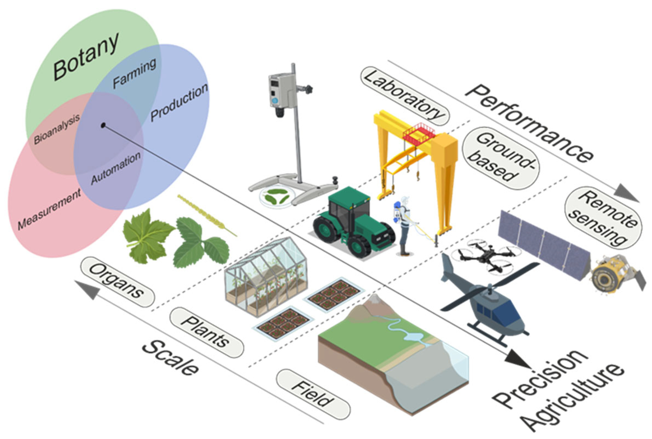
:1. Introduction
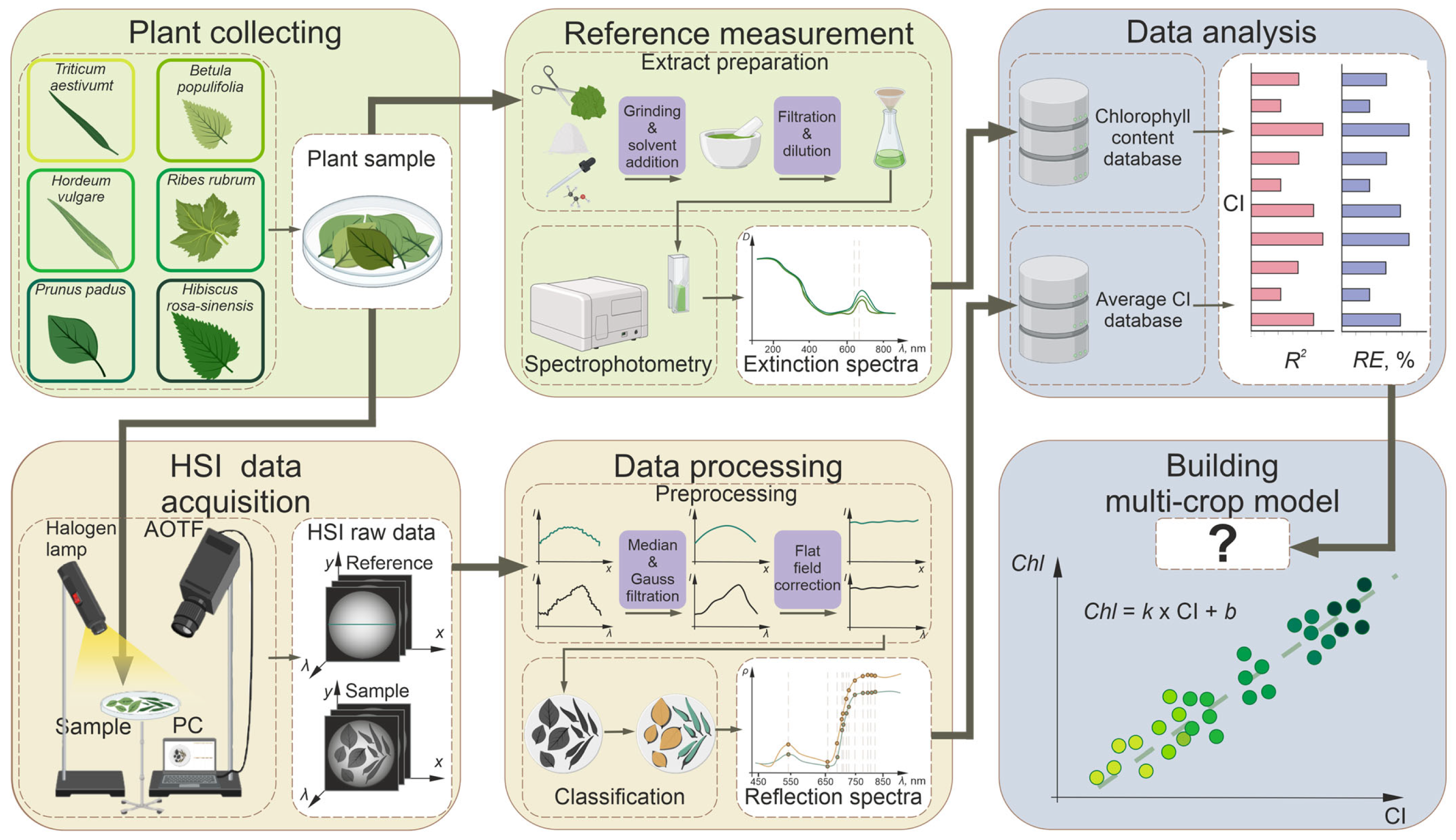
2. Materials and Methods
2.1. Experimental Plants
2.2. Experimental Protocol
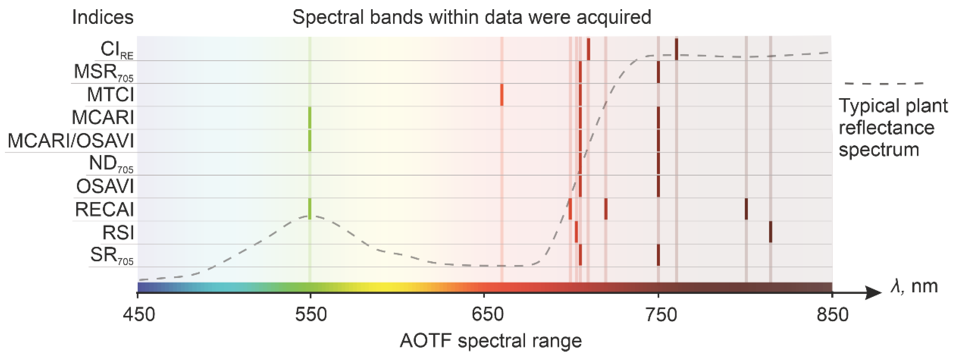
2.3. Selection of Spectral Bands
2.4. Model Evaluation
3. Results
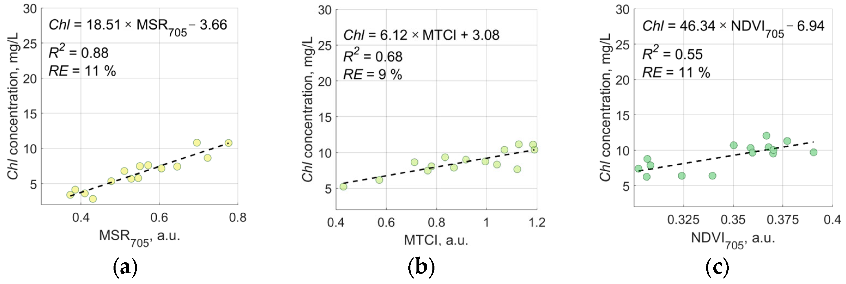
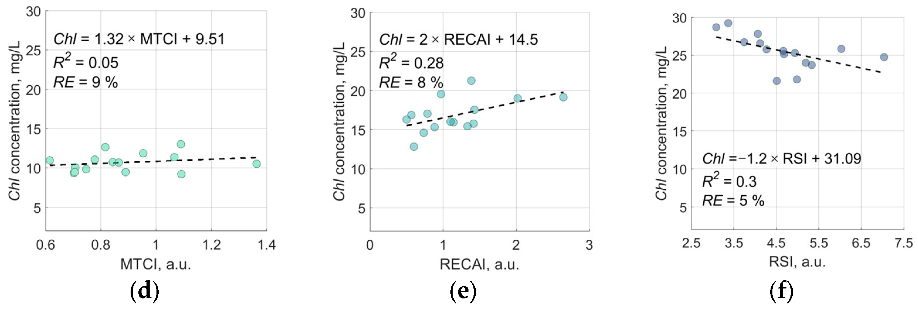
3.1. Single-Crop Models
3.2. Multi-Crop Model
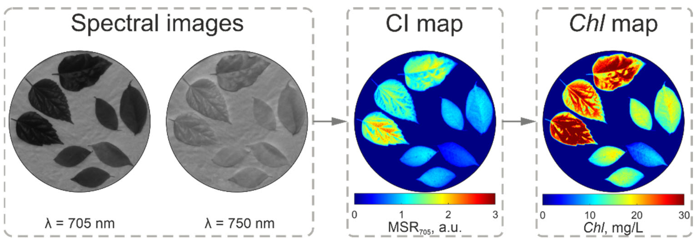
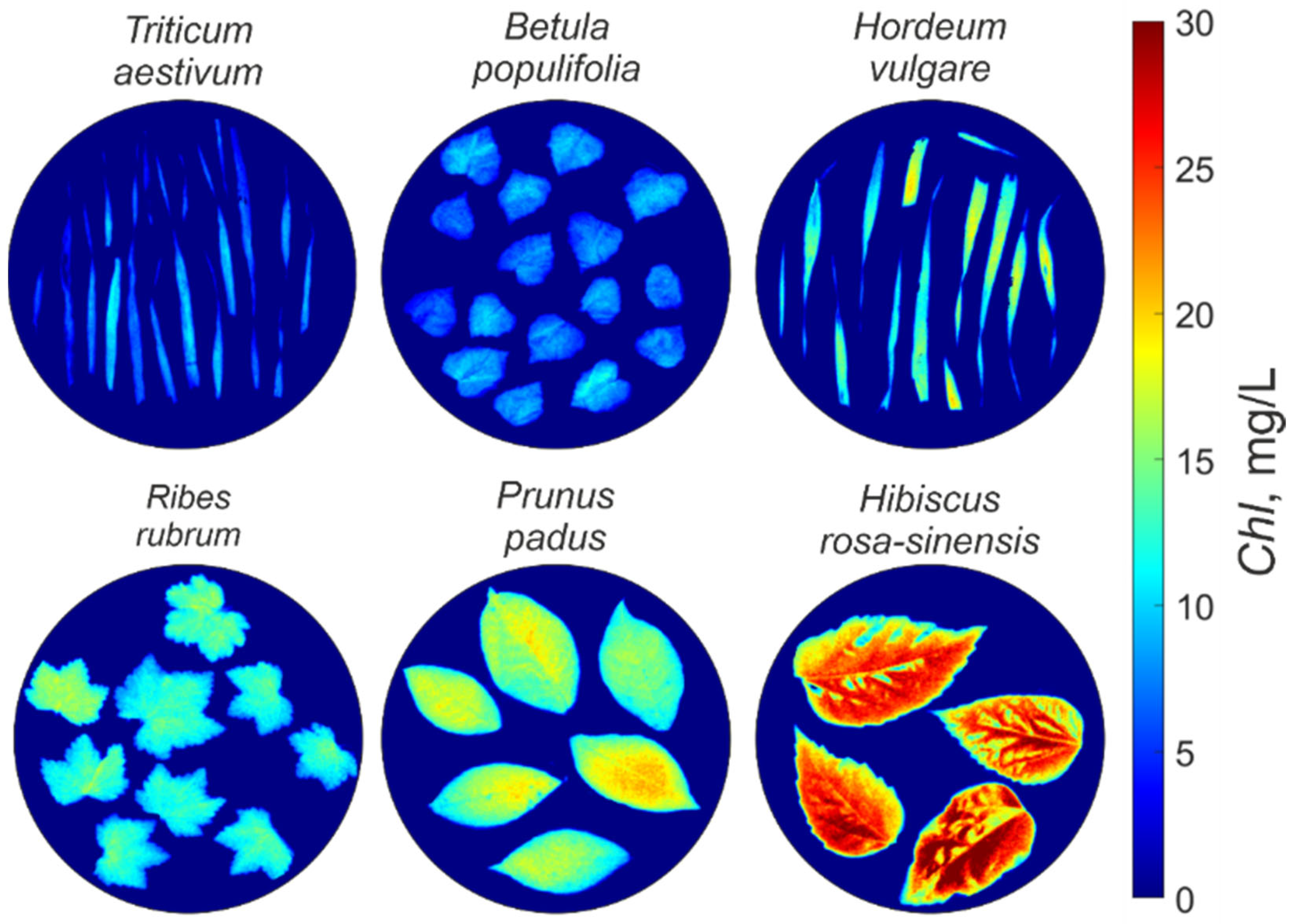
3.3. Chlorophyll Mapping
4. Discussion
5. Conclusions
Author Contributions
Funding
Data Availability Statement
Acknowledgments
Conflicts of Interest
Appendix A

| Crop | Triticum aestivum | Betula populifolia | Hordeum vulgare | Ribes rubrum | Prunus padus | Hibiscus rosa-sinensis | Multi-Crop |
|---|---|---|---|---|---|---|---|
| 0.86 ± 0.63 | 0.75 ± 0.57 | 0.78 ± 0.3 | 0.71 ± 0.51 | 1.18 ± 0.8 | 2.19 ± 0.45 | 1.08 ± 1.67 | |
| 0.55 ± 0.37 | 0.61 ± 0.39 | 0.61 ± 0.2 | 0.59 ± 0.32 | 0.89 ± 0.49 | 1.4 ± 0.24 | 0.77 ± 0.97 | |
| 0.82 ± 0.83 | 0.91 ± 0.68 | 0.85 ± 0.36 | 0.88 ± 0.6 | 1.56 ± 1.29 | 2.63 ± 0.75 | 1.27 ± 2.13 | |
| 0.56 ± 0.53 | 0.7 ± 0.57 | 0.77 ± 0.28 | 0.66 ± 0.51 | 1.18 ± 0.9 | 2.13 ± 0.71 | 1 ± 1.74 | |
| 1.67 ± 0.75 | 1.94 ± 0.7 | 2.12 ± 0.27 | 1.87 ± 0.63 | 2.48 ± 0.95 | 3.43 ± 0.81 | 2.25 ± 1.89 | |
| 0.32 ± 0.17 | 0.34 ± 0.18 | 0.35 ± 0.09 | 0.34 ± 0.14 | 0.46 ± 0.18 | 0.61 ± 0.06 | 0.4 ± 0.35 | |
| 0.33 ± 0.17 | 0.36 ± 0.18 | 0.36 ± 0.09 | 0.35 ± 0.14 | 0.47 ± 0.18 | 0.62 ± 0.07 | 0.41 ± 0.34 | |
| 0.92 ± 0.75 | 0.47 ± 0.7 | 0.45 ± 0.4 | 0.33 ± 0.57 | 1.17 ± 1.74 | 2.73 ± 1.36 | 1.01 ± 2.68 | |
| 2.30 ± 1.06 | 2.22 ± 1.3 | 1.95 ± 0.96 | 1.91 ± 0.95 | 3.19 ± 2.74 | 4.67 ± 3.03 | 2.71 ± 3.46 | |
| 1.95 ± 0.77 | 2.07 ± 0.8 | 2.07 ± 0.41 | 2.03 ± 0.68 | 2.73 ± 1.26 | 4.18 ± 0.78 | 2.51 ± 2.52 |
References
- Rockström, J.; Williams, J.; Daily, G.; Noble, A.; Matthews, N.; Gordon, L.; Wetterstrand, H.; DeClerck, F.; Shah, M.; Steduto, P.; et al. Sustainable Intensification of Agriculture for Human Prosperity and Global Sustainability. Ambio 2017, 46, 4–17. [Google Scholar] [CrossRef]
- Hunter, M.C.; Smith, R.G.; Schipanski, M.E.; Atwood, L.W.; Mortensen, D.A. Agriculture in 2050: Recalibrating Targets for Sustainable Intensification. Bioscience 2017, 67, 386–391. [Google Scholar] [CrossRef]
- Gebbers, R.; Adamchuk, V.I. Precision Agriculture and Food Security. Science 2010, 327, 828–831. [Google Scholar] [CrossRef]
- Majumdar, J.; Naraseeyappa, S.; Ankalaki, S. Analysis of Agriculture Data Using Data Mining Techniques: Application of Big Data. J. Big Data 2017, 4, 20. [Google Scholar] [CrossRef]
- Féret, J.B.; Gitelson, A.A.; Noble, S.D.; Jacquemoud, S. PROSPECT-D: Towards Modeling Leaf Optical Properties through a Complete Lifecycle. Remote Sens. Environ. 2017, 193, 204–215. [Google Scholar] [CrossRef]
- Roper, J.M.; Garcia, J.F.; Tsutsui, H. Emerging Technologies for Monitoring Plant Health in Vivo. ACS Omega 2021, 6, 5101–5107. [Google Scholar] [CrossRef] [PubMed]
- Barbedo, J.G.A. A Review on the Use of Unmanned Aerial Vehicles and Imaging Sensors for Monitoring and Assessing Plant Stresses. Drones 2019, 3, 40. [Google Scholar] [CrossRef]
- Gitelson, A.A.; Peng, Y.; Arkebauer, T.J.; Schepers, J. Relationships between Gross Primary Production, Green LAI, and Canopy Chlorophyll Content in Maize: Implications for Remote Sensing of Primary Production. Remote Sens. Environ. 2014, 144, 65–72. [Google Scholar] [CrossRef]
- Benelli, A.; Cevoli, C.; Fabbri, A. In-Field Hyperspectral Imaging: An Overview on the Ground-Based Applications in Agriculture. J. Agric. Eng. 2020, 51, 129–139. [Google Scholar] [CrossRef]
- Lu, B.; Dao, P.D.; Liu, J.; He, Y.; Shang, J. Recent Advances of Hyperspectral Imaging Technology and Applications in Agriculture. Remote Sens. 2020, 12, 2659. [Google Scholar] [CrossRef]
- Mulla, D.J. Twenty Five Years of Remote Sensing in Precision Agriculture: Key Advances and Remaining Knowledge Gaps. Biosyst. Eng. 2013, 114, 358–371. [Google Scholar] [CrossRef]
- Kwan, C. Remote Sensing Performance Enhancement in Hyperspectral Images. Sensors 2018, 18, 3598. [Google Scholar] [CrossRef]
- Sethy, P.K.; Pandey, C.; Sahu, Y.K.; Behera, S.K. Hyperspectral Imagery Applications for Precision Agriculture—A Systemic Survey. Multimed. Tools Appl. 2021, 81, 3005–3038. [Google Scholar] [CrossRef]
- Li, P.; Wang, Q. Retrieval of Chlorophyll for Assimilating Branches of a Typical Desert Plant through Inversed Radiative Transfer Models. Int. J. Remote Sens. 2013, 34, 2402–2416. [Google Scholar] [CrossRef]
- Vohland, M.; Jarmer, T. Estimating Structural and Biochemical Parameters for Grassland from Spectroradiometer Data by Radiative Transfer Modelling (PROSPECT+SAIL). Int. J. Remote Sens. 2008, 29, 191–209. [Google Scholar] [CrossRef]
- Sehgal, V.K.; Chakraborty, D.; Sahoo, R.N. Inversion of Radiative Transfer Model for Retrieval of Wheat Biophysical Parameters from Broadband Reflectance Measurements. Inf. Process. Agric. 2016, 3, 107–118. [Google Scholar] [CrossRef]
- Cheng, J.; Yang, H.; Qi, J.; Sun, Z.; Han, S.; Feng, H.; Jiang, J.; Xu, W.; Li, Z.; Yang, G.; et al. Estimating Canopy-Scale Chlorophyll Content in Apple Orchards Using a 3D Radiative Transfer Model and UAV Multispectral Imagery. Comput. Electron. Agric. 2022, 202, 107401. [Google Scholar] [CrossRef]
- Berger, K.; Verrelst, J.; Féret, J.B.; Hank, T.; Wocher, M.; Mauser, W.; Camps-Valls, G. Retrieval of Aboveground Crop Nitrogen Content with a Hybrid Machine Learning Method. Int. J. Appl. Earth Obs. Geoinf. 2020, 92, 102174. [Google Scholar] [CrossRef]
- Verrelst, J.; Camps-Valls, G.; Muñoz-Marí, J.; Rivera, J.P.; Veroustraete, F.; Clevers, J.G.P.W.; Moreno, J. Optical Remote Sensing and the Retrieval of Terrestrial Vegetation Bio-Geophysical Properties—A Review. ISPRS J. Photogramm. Remote Sens. 2015, 108, 273–290. [Google Scholar] [CrossRef]
- Lu, B.; He, Y. Evaluating Empirical Regression, Machine Learning, and Radiative Transfer Modelling for Estimating Vegetation Chlorophyll Content Using Bi-Seasonal Hyperspectral Images. Remote Sens. 2019, 11, 1979. [Google Scholar] [CrossRef]
- Li, J.; Wijewardane, N.K.; Ge, Y.; Shi, Y. Improved Chlorophyll and Water Content Estimations at Leaf Level with a Hybrid Radiative Transfer and Machine Learning Model. Comput. Electron. Agric. 2023, 206, 107669. [Google Scholar] [CrossRef]
- Haboudane, D.; Miller, J.R.; Tremblay, N.; Zarco-Tejada, P.J.; Dextraze, L. Integrated Narrow-Band Vegetation Indices for Prediction of Crop Chlorophyll Content for Application to Precision Agriculture. Remote Sens. Environ. 2002, 81, 416–426. [Google Scholar] [CrossRef]
- Zeng, Y.; Hao, D.; Huete, A.; Dechant, B.; Berry, J.; Chen, J.M.; Joiner, J.; Frankenberg, C.; Bond-Lamberty, B.; Ryu, Y.; et al. Optical Vegetation Indices for Monitoring Terrestrial Ecosystems Globally. Nat. Rev. Earth Environ. 2022, 3, 477–493. [Google Scholar] [CrossRef]
- Bannari, A.; Morin, D.; Bonn, F.; Huete, A.R. A Review of Vegetation Indices. Remote Sens. Rev. 1995, 13, 95–120. [Google Scholar] [CrossRef]
- Ma, Y.; Zhang, Q.; Yi, X.; Ma, L.; Zhang, L.; Huang, C.; Zhang, Z.; Lv, X. Estimation of Cotton Leaf Area Index (LAI) Based on Spectral Transformation and Vegetation Index. Remote Sens. 2021, 14, 136. [Google Scholar] [CrossRef]
- Inoue, Y.; Penueleus, J.; Nouevllon, Y.; Moran, M.S. Hyperspectral Reflectance Measurements for Estimating Eco-Physiological Status of Plants. In Hyperspectral Remote Sensing of the Land and Atmosphere; SPIE: Bellingham, WA, USA, 2001; Volume 4151, pp. 153–163. [Google Scholar] [CrossRef]
- Inoue, Y.; Penuelas, J. An AOTF-Based Hyperspectral Imaging System for Field Use in Ecophysiological and Agricultural Applications. Int. J. Remote Sens. 2010, 22, 3883–3888. [Google Scholar] [CrossRef]
- Slovin, J.P.; Bandurski, R.S.; Cohen, J.D. Chapter 5 Auxin. New Compr. Biochem. 1999, 33, 115–140. [Google Scholar] [CrossRef]
- Calpe-Maravilla, J.; Vila-Frances, J.; Ribes-Gomez, E.; Duran-Bosch, V.; Munoz-Mari, J.; Amoros-Lopez, J.; Gomez-Chova, L.; Tajahuerce-Romera, E. 400- to 1000-Nm Imaging Spectrometer Based on Acousto-Optic Tunable Filters. In Sensors, Systems, and Next-Generation Satellites VIII; SPIE: Bellingham, WA, USA, 2004; Volume 5570, p. 460. [Google Scholar] [CrossRef]
- Zolotukhina, A.; Machikhin, A.; Guryleva, A.; Gresis, V.; Tedeeva, V. Extraction of Chlorophyll Concentration Maps from AOTF Hyperspectral Imagery. Front. Environ. Sci. 2023, 11, 480. [Google Scholar] [CrossRef]
- Pyakurel, A.; Wang, J.R. Leaf Morphological Variation among Paper Birch (Betula papyrifera Marsh.) Genotypes across Canada. Open J. Ecol. 2013, 03, 284–295. [Google Scholar] [CrossRef]
- Leather, S.R. Prunus padus L. J. Ecol. 1996, 84, 125. [Google Scholar] [CrossRef]
- Siregar, A.Y.; Salamah, A. Variation of Leaf Morphology of Hibiscus Rosa-Sinensis L. under Various Light Intensities at Universitas Indonesia Campus Area and Citayam, Depok. In IOP Conference Series: Earth and Environmental Science; IOP Publishing: Bristol, UK, 2020; Volume 524. [Google Scholar] [CrossRef]
- Chitwood, D.H.; Sinha, N.R. Evolutionary and Environmental Forces Sculpting Leaf Development. Curr. Biol. 2016, 26, R297–R306. [Google Scholar] [CrossRef] [PubMed]
- Pustovoit, V.I.; Pozhar, V.E.; Mazur, M.M.; Shorin, V.N.; Kutuza, I.B.; Perchik, A.V. Double-AOTF Spectral Imaging System. In Acousto-Optics and Photoacoustics; SPIE: Bellingham, WA, USA, 2005; Volume 5953, pp. 200–203. [Google Scholar] [CrossRef]
- Pu, R. Hyperspectral Remote Sensing: Fundamentals and Practices; CRC Press: Boca Raton, FL, USA, 2017; pp. 1–466. [Google Scholar]
- Padma, S.; Sanjeevi, S. Jeffries Matusita-Spectral Angle Mapper (JM-SAM) Spectral Matching for Species Level Mapping at Bhitarkanika, Muthupet and Pichavaram Mangroves. Int. Arch. Photogramm. Remote Sens. Spat. Inf. Sci. 2014, XL–8, 1403–1411. [Google Scholar] [CrossRef]
- Wintermans, J.F.G.M.; De Mots, A. Spectrophotometric Characteristics of Chlorophylls a and b and Their Phenophytins in Ethanol. Biochim. Biophys. Acta (BBA)—Biophys. Incl. Photosynth. 1965, 109, 448–453. [Google Scholar] [CrossRef]
- Gitelson, A.A.; Viña, A.; Ciganda, V.; Rundquist, D.C.; Arkebauer, T.J. Remote Estimation of Canopy Chlorophyll Content in Crops. Geophys. Res. Lett. 2005, 32, L08403. [Google Scholar] [CrossRef]
- Wu, C.; Niu, Z.; Tang, Q.; Huang, W. Estimating Chlorophyll Content from Hyperspectral Vegetation Indices: Modeling and Validation. Agric. For. Meteorol. 2008, 148, 1230–1241. [Google Scholar] [CrossRef]
- Dash, J.; Curran, P.J. The MERIS Terrestrial Chlorophyll Index. Int. J. Remote Sens. 2004, 25, 5403–5413. [Google Scholar] [CrossRef]
- Sims, D.A.; Gamon, J.A. Relationships between Leaf Pigment Content and Spectral Reflectance across a Wide Range of Species, Leaf Structures and Developmental Stages. Remote Sens. Environ. 2002, 81, 337–354. [Google Scholar] [CrossRef]
- Yuhao, A.; Norasma, N.; Ya, C.; Roslin, A.; Ismail, M.R. SCIENCE & TECHNOLOGY Rice Chlorophyll Content Monitoring Using Vegetation Indices from Multispectral Aerial Imagery. Pertanika J. Sci. Technol. 2020, 28, 779–795. [Google Scholar]
- Fern, R.R.; Foxley, E.A.; Bruno, A.; Morrison, M.L. Suitability of NDVI and OSAVI as Estimators of Green Biomass and Coverage in a Semi-Arid Rangeland. Ecol. Indic. 2018, 94, 16–21. [Google Scholar] [CrossRef]
- Cui, B.; Zhao, Q.; Huang, W.; Song, X.; Ye, H.; Zhou, X. A New Integrated Vegetation Index for the Estimation of Winter Wheat Leaf Chlorophyll Content. Remote Sens. 2019, 11, 974. [Google Scholar] [CrossRef]
- Laroche-Pinel, E.; Albughdadi, M.; Duthoit, S.; Chéret, V.; Rousseau, J.; Clenet, H. Understanding Vine Hyperspectral Signature through Different Irrigation Plans: A First Step to Monitor Vineyard Water Status. Remote Sens. 2021, 13, 536. [Google Scholar] [CrossRef]
- Inoue, Y.; Guérif, M.; Baret, F.; Skidmore, A.; Gitelson, A.; Schlerf, M.; Darvishzadeh, R.; Olioso, A. Simple and Robust Methods for Remote Sensing of Canopy Chlorophyll Content: A Comparative Analysis of Hyperspectral Data for Different Types of Vegetation. Plant Cell Environ. 2016, 39, 2609–2623. [Google Scholar] [CrossRef] [PubMed]
- Evain, S.; Flexas, J.; Moya, I. A New Instrument for Passive Remote Sensing: 2. Measurement of Leaf and Canopy Reflectance Changes at 531 Nm and Their Relationship with Photosynthesis and Chlorophyll Fluorescence. Remote Sens. Environ. 2004, 91, 175–185. [Google Scholar] [CrossRef]
- Gilman, E.L.; Ellison, J.; Duke, N.C.; Field, C. Threats to Mangroves from Climate Change and Adaptation Options: A Review. Aquat. Bot. 2008, 89, 237–250. [Google Scholar] [CrossRef]
- Carter, G.A.; Knapp, A.K. Leaf Optical Properties in Higher Plants: Linking Spectral Characteristics to Stress and Chlorophyll Concentration. Am. J. Bot. 2001, 88, 677–684. [Google Scholar] [CrossRef] [PubMed]
- Darvishzadeh, R.; Skidmore, A.; Schlerf, M.; Atzberger, C. Inversion of a Radiative Transfer Model for Estimating Vegetation LAI and Chlorophyll in a Heterogeneous Grassland. Remote Sens. Environ. 2008, 112, 2592–2604. [Google Scholar] [CrossRef]
- Darvishzadeh, R.; Skidmore, A.; Schlerf, M.; Atzberger, C.; Corsi, F.; Cho, M. LAI and Chlorophyll Estimation for a Heterogeneous Grassland Using Hyperspectral Measurements. ISPRS J. Photogramm. Remote Sens. 2008, 63, 409–426. [Google Scholar] [CrossRef]
- Katrašnik, J.; Bürmen, M.; Pernuš, F.; Likar, B. Spectral Characterization and Calibration of AOTF Spectrometers and Hyper-Spectral Imaging Systems. Chemom. Intell. Lab. Syst. 2010, 101, 23–29. [Google Scholar] [CrossRef]
- Martynov, G.N.; Pozhar, V.E.; Gorevoy, A.V.; Machikhin, A.S. Spatiospectral Transformation of Noncollimated Light Beams Diffracted by Ultrasound in Birefringent Crystals. Photonics Res. 2021, 9, 687–693. [Google Scholar] [CrossRef]


| Crop | Plant Functional Type | Length of Leaf Blade, mm | Width of Leaf Blade, mm | Form of Leaf Blade | Cover of Leaf Blade | Pubescence | Leaf Venation | CC, mg/L |
|---|---|---|---|---|---|---|---|---|
| Triticum aestivum | Annual | <300 | 10–20 | Lanceolar | Smooth, scabrous | No | Parallel | 3.9–9.9 |
| Betula populifolia | Drought deciduous | 50–70 | 40–60 | Oval | Smooth, scabrous | Yes | Pinnate, dictyodromous | 3.5–13.2 |
| Hordeum vulgare | Annual | <300 | 20–30 | Lanceolar | Smooth, scabrous | No | Parallel | 4.2–9.9 |
| Ribes rubrum | Drought deciduous | 20–50 | <120 | Lobar-digitate | Smooth, scabrous | Yes | Dictyodromous | 9.8–16.1 |
| Prunus padus | Drought deciduous | 60–130 | 35–60 | Oval-lanceolar | Smooth, scabrous | Yes | Pinnate | 1.7–5.5 |
| Hibiscus rosa-sinensis | Evergreen perennial | 50–120 | 30–85 | Oval-digitate | Smooth, glossy | No | Dictyodromous | 7.8–39.2 |
| Crop | Collection Point | Collection Date | Developmental Stage | Soil Type | Conditions | Organic Material, % | P2O5, mg/kg | K2O, mg/kg |
|---|---|---|---|---|---|---|---|---|
| Triticum aestivum | 57.775713, 56.329550 | 7 May 2023 | Mature | Sod-podzolic | Field | 2.9 | 2.45–5.75 | 9–40.95 |
| Betula populifolia | 55.954216, 37.944919 | 11 May 2023 | Mature | 3.5 | 10.15 | 52.67 | ||
| Hordeum vulgare | 57.837534, 56.302138 | 9 May 2023 | Mature | 2.43 | 1.633 | 38.73 | ||
| Ribes rubrum | 55.953855, 37.944774 | 11 May 2023 | Expanding | 4 | 16.34 | 57.14 | ||
| Prunus padus | 55.951942, 37.943452 | 19 May 2023 | Mature | 3.5 | 10.15 | 52.67 | ||
| Hibiscus rosa-sinensis | 55.942252, 37.951099 | 19 May 2023 | Senescing | Artificial soil | Laboratory | 10 | 30 | 100 |
| Parameter | Value |
|---|---|
| Spectral tuning range, nm | 450–850 |
| Tuning time, μs | 10 |
| Accuracy of spectral access, nm | 0.1 |
| Spectral resolution, nm | 3.5 nm (at 532 nm) |
| Spatial resolution, pixels | 500 × 500 |
| Field of view, ° | 15 × 20 |
| Working distance, m | 1 − ∞ |
| Frame rate | up to 100 images/s |
| Crop | Reference CC, mg/L |
|---|---|
| Triticum aestivum | 6.50 ± 2.45 |
| Betula populifolia | 8.64 ± 1.69 |
| Hordeum vulgare | 9.12 ± 1.86 |
| Ribes rubrum | 10.67 ± 1.18 |
| Prunus padus | 16.83 ± 2.17 |
| Hibiscus rosa-sinensis | 25.49 ± 2.19 |
| Chlorophyll Index | Definition | Inspected Crops | Reference |
|---|---|---|---|
| Red-Edge Chlorophyll Index | Maize, soybean | [39] | |
| Modified Simple Ratio | Winter wheat, eared, no-eared corn | [40] | |
| MERIS terrestrial chlorophyll index | Fir, maple | [41] | |
| Modified Chlorophyll Absorption Ratio Index | Winter wheat, eared and no-eared corn | [40] | |
| Winter wheat, eared and no-eared corn | [40] | ||
| Normalized Difference Vegetation Index | Herbaceous, sclerophyllous, succulent, grasses and others (53 species) | [42] | |
| Optimized Soil-Adjusted Vegetation Index | Rice, woody plants, dense shrubs, cacti | [43,44] | |
| Red-Edge Chlorophyll Absorption Index | Winter wheat, grape | [45,46] | |
| Ratio spectral index | Rice, wheat, corn, soybean, sugar beet and grass | [47] | |
| Herbaceous, sclerophyllous, succulent, grasses and others (53 species) | [42] |
| Regression Type | Regression Model | ||
|---|---|---|---|
| Linear | Chl = 19.87 × MSR705 − 2.49 | 0.89 | 15 |
| Polynomial (n = 2) | Chl = 54.82 × (NDVI705)2 + 6.34 × NDVI705 + 0.72 | 0.89 | 14.46 |
| Polynomial (n = 3) | Chl = −0.17 × (NDVI705)3 + 0.54 × (NDVI705)2 + 9.18 × NDVI705 − 10.26 | 0.89 | 14.41 |
| Power | Chl = 17.15 × (MSR705)1.17 | 0.89 | 14.46 |
| Exponential | Chl = 2.66 × exp(3.68 × NDVI705) | 0.89 | 14.91 |
| Logarithmic | Chl = 21.69 × exp(0.75 × SR705) | 0.89 | 14.57 |
| Multiple linear | Chl = 18.99 + 102.53 × MSR705 − 94.34 × NDVI705 − 18.91 × SR705 | 0.89 | 14.44 |
| Chl = −2.65 + 19.41 × MSR705 + 1.30 × NDVI705 | 0.89 | 14.55 | |
| Chl = −7.72 + 23.90 × NDVI705 + 4.38 × SR705 | 0.89 | 14.57 |
Disclaimer/Publisher’s Note: The statements, opinions and data contained in all publications are solely those of the individual author(s) and contributor(s) and not of MDPI and/or the editor(s). MDPI and/or the editor(s) disclaim responsibility for any injury to people or property resulting from any ideas, methods, instructions or products referred to in the content. |
© 2024 by the authors. Licensee MDPI, Basel, Switzerland. This article is an open access article distributed under the terms and conditions of the Creative Commons Attribution (CC BY) license (https://creativecommons.org/licenses/by/4.0/).
Share and Cite
Zolotukhina, A.; Machikhin, A.; Guryleva, A.; Gresis, V.; Kharchenko, A.; Dekhkanova, K.; Polyakova, S.; Fomin, D.; Nesterov, G.; Pozhar, V. Evaluation of Leaf Chlorophyll Content from Acousto-Optic Hyperspectral Data: A Multi-Crop Study. Remote Sens. 2024, 16, 1073. https://doi.org/10.3390/rs16061073
Zolotukhina A, Machikhin A, Guryleva A, Gresis V, Kharchenko A, Dekhkanova K, Polyakova S, Fomin D, Nesterov G, Pozhar V. Evaluation of Leaf Chlorophyll Content from Acousto-Optic Hyperspectral Data: A Multi-Crop Study. Remote Sensing. 2024; 16(6):1073. https://doi.org/10.3390/rs16061073
Chicago/Turabian StyleZolotukhina, Anastasia, Alexander Machikhin, Anastasia Guryleva, Valeria Gresis, Anastasia Kharchenko, Karina Dekhkanova, Sofia Polyakova, Denis Fomin, Georgiy Nesterov, and Vitold Pozhar. 2024. "Evaluation of Leaf Chlorophyll Content from Acousto-Optic Hyperspectral Data: A Multi-Crop Study" Remote Sensing 16, no. 6: 1073. https://doi.org/10.3390/rs16061073