AIDB-Net: An Attention-Interactive Dual-Branch Convolutional Neural Network for Hyperspectral Pansharpening

Abstract

Despite notable advancements achieved on Hyperspectral (HS) pansharpening tasks through deep learning techniques, previous methods are inherently constrained by convolution or self-attention intrinsic defects, leading to limited performance. In this paper, we proposed an Attention-Interactive Dual-Branch Convolutional Neural Network (AIDB-Net) for HS pansharpening. Our model purely consists of convolutional layers and simultaneously inherits the strengths of both convolution and self-attention, especially the modeling of short- and long-range dependencies. Specially, we first extract, tokenize, and align the hyperspectral image (HSI) and panchromatic image (PAN) by Overlapping Patch Embedding Blocks. Then, we specialize a novel Spectral-Spatial Interactive Attention which is able to globally interact and fuse the cross-modality features. The resultant token-global similarity scores can guide the refinement and renewal of the textural details and spectral characteristics within HSI features. By deeply combined these two paradigms, our AIDB-Net significantly improve the pansharpening performance. Moreover, with the acceleration by the convolution inductive bias, our interactive attention can be trained without large scale dataset and achieves competitive time cost with its counterparts. Compared with the state-of-the-art methods, our AIDB-Net makes 5.2%, 3.1%, and 2.2% improvement on PSNR metric on three public datasets, respectively. Comprehensive experiments quantitatively and qualitatively demonstrate the effectiveness and superiority of our AIDB-Net.

1. Introduction

With the rapid development of remote sensing technologies, remote sensing images are gradually becoming versatile and have been widely applied in many domains: including scene classification [1], target detection [2], denoising [3], and spectral unmixing [4]. There are two commonly prevalent categories remote sensing images: hyperspectral image (HSI) and panchromatic image (PAN). The HSI records abundant spectral information by densely sampling dozens or even hundreds of continuous spectral bands from visible to infrared wavelengths. The extensive spectral coverage empowers the identification of various materials on Earth through spectral signatures [5]. However, the spatial resolution of HSI is low. In contrast to HSI, PAN excel in recording the elaborate textural details of ground objects within a single spectral band. Restricted by the hardware limitations, the hyperspectral imaging system cannot captures a remote sensing images with both high spectral and spatial quality. The cost of high spectral resolution for HSI is blurry textural details. The absence of spatial information in HSI significantly hinders its application potential. Therefore, it becomes imperative to leverage super-resolution techniques to enhance the spatial resolution of HSI. These methods can be broadly categorized into two types: single-image super-resolution (SISR) and multi-image super-resolution (MISR) [6]. While SISR applies the super-resolution algorithm solely to a single HSI without auxiliary PAN, MISR boosts the spatial resolution of HSI by incorporating the refined textural details from PAN. This integration often yields superior super-resolution performance in terms of both spectral and spatial fidelity. In general, MISR is commonly referred as hyperspectral (HS) pansharpening by the official.

To obtain high spatial resolution HSI, numerous pansharpening approaches have been proposed over the past few decades, which can be divided into traditional and emerging methods. Among traditional methods, component substitution (CS)-based methods depend on replacement of the spatial component of the source HSI with the corresponding PAN, which includes Intensity-Hue-Saturation (IHS) [7], Brovey [8], Principal Component Analysis (PCA) [9], Gram-Schmidt (GS) [10], and Gram-Schmidt Adaptive (GSA) [11]. While CS-based methods effectively achieve the transmission of the spatial information from PAN to HSI, they often introduce spectral distortions in the pansharpened image. In contrast, multi resolution analysis (MRA)-based methods begin by decomposing the source HSI and PAN into different scales using a multi-scale decomposition algorithm. Subsequently, the spectral and spatial features are fused within each scale. The family of MRA-based methods mainly involve Smoothing Filter-based Intensity Modulation (SFIM) [12], Generalized Laplacian Pyramid (GLP) with Modulation Transfer Function (MTF) matched filter (MTF-GLP) [13], MTF-GLP with High-Pass Modulation (MTF-GLP-HPM) [14]. Unlike CS-based methods, MRA-based methods demonstrate superior performance in spectral preservation, albeit at the expense of introducing spatial distortions in the pansharpened image. In addition to these purely CS- or MRA-based methods, hybrid approaches for HS pansharpening have also been studied. Examples include guided filter PCA (GFPCA) [15], which simultaneously inherit the advantages of both CS- and MRA-based methods. In addition to above approaches, variational optimization (VO)-based methods approach HS pansharpening as an optimization problem, formulating a constrained objective function with prior knowledge derived from the source HSI, PAN, and the ideal HSI. Interactive optimization algorithms are typically employed to find suitable solutions. Representative examples include Coupled Non-negative Matrix Factorization (CNMF) [16], Convex Regularization under a Bayesian Gaussian prior (HySure) [17], and naive Bayesian Gaussian prior (BF) [18]. While VO-based methods yield relatively high pansharpening quality, they are often characterized by slow processing speeds and challenging fine-tuning requirements.

The advantages and shortcomings of different categories HS pansharpening methods have been represented in

Table 1. Advantages and shortcomings of different kinds of HS pansharpening methods.

Category	Advantage	Shortcoming
CS	Better spatial reconstruction Easy to use	Distort the spectral features Sensitive to the scale ratio and sensor type
MRA	Better spectral preservation Easy to use	Distort the spatial features Sensitive to the scale ratio and misregistration
HYBRID	Insensitive to the scale ratio and misregistration	Distort the spectral and spatial features
VO	Better spectral preservation and spatial reconstruction	Relatively slow Hard to fine tune
DL	Fast (pre-trained model) Better spectral preservation and spatial reconstruction	Hardware demanding Hard to pre-train and fine tune Depend on large scale dataset

. In a word, traditional methods often suffer from inadequate representation ability or inappropriate assumptions, resulting in notable spectral and spatial distortions in the pansharpened image.

In recent years, deep learning (DL)-based methods, especially convolutional neural network (CNN), gradually emerge as a transformative solution for HS pansharpening. Leveraging their powerful capabilities of feature extraction and nonlinear optimization, CNN-based methods have already achieved state-of-the-art (SOTA) performance. Following the design philosophy of natural image super-resolution, Masi et al. [19] introduced a pansharpening neural network (PNN) comprising three convolutional layers as an initial attempt. However, the performance of PNN is constrained due to its simple architecture and less parameters. Yang et al. [20] developed PanNet, a pansharpening neural network that incorporates domain-specific knowledge, emphasizing both spectral preservation and spatial enhancement. To achieve spectral preservation, PanNet employs a direct propagation of spectral information through a summation operation between the up-sampled multispectral and reconstructed image. For spatial enhancement, PanNet is trained in the high-pass filtering domain rather than image domain. A lot of CNN-based methods [21,22,23,24] have been proposed to address HS pansharpening problem, achieving impressive performance. With the growing recognition of both convolution and HS pansharpening, the dual-branch design paradigm has emerged as a common approach. This paradigm involves the parallel processing of spectral and spatial information on two branches, followed by the integration of advanced spatial information into the spectral features through specially designed aggregation component. He et al. [25] introduced HyperPNN, a spectrally predictive convolutional neural network designed for HS pansharpening. HyperPNN comprises two sub-networks: a spectral prediction sub-network dedicated to spectral prediction and a spatial-spectral inference sub-network aimed at leveraging both spectral and spatial contextual information. Wang et al. [5] proposed a dual-path fusion network (DPFN) designed to capture both global spectral-spatial and local high-pass spatial information through two distinct learning paths. The model is trained using a combinatorial loss function, which includes pixel-wise mean square error (MSE) and feature-wise near-infrared-VGG loss, aiming to enhance performance. Qu [26] proposed a dual-branch detail extraction pansharpening network (DBDENet) that can solve the pansharpening problem with any number of spectral bands. However, 2D CNNs are primarily adept at capturing spatial information along the width and height dimensions, making it challenging to preserve the spectral features of HSI data cubes. To address this limitation, Zheng et al. [27] introduced an edge-conditioned feature transform network (EC-FTN) that utilizes 3D convolutional layers. This design enables the joint extraction of spectral and spatial features from HSI, resulting in the preservation of fine details and high spectral fidelity.

Despite the numerous CNN-based methods proposed for HS pansharpening, two critical issues persist:

• Cross-Modality Dependency Modeling: In order to fuse the diverse modality information, most CNN-based methods often concatenate HSI with PAN in either the image domain or feature domain. However, concatenating a single spectral band PAN with dozens or even hundreds of spectral bands HSI fails to properly model the cross-modality dependencies between them.
• Limited Exploitation of Global Information: CNN-based methods, constrained by their receptive field, typically focus on extracting local information from the input image. Unfortunately, this approach neglects the importance of global information. However, both local and global information are crucial for accurate pansharpening.

In addition to convolution, another emerging DL model, the transformer architecture, has shown promising prospect in computer vision community. Transformer exclusively relies on the self-attention mechanism, which enables the adjustment of each pixel based on the long-range dependencies of input features. Researchers have begun exploring transformer-based pansharpening model and there already exists some relevant works in the community. Meng et al. [28] introduced a modified Vision Transformer (ViT) [29] style model for HS pansharpening. Chaminda Bandara et al. [30] proposed HyperTransformer, a textural-spectral feature fusion transformer. In HyperTransformer, an improved self-attention mechanism is designed to identify spectrally similar and texturally superior features for source HSI. Notably, the features of low spatial resolution HSI, down-sampled PAN, and PAN are formulated as Query, Key, and Value, respectively. HyperTransformer can extract cross-modality dependencies in a global manner, which is completely different to convolution. Moreover, Fusformer [31] and Panformer [32] have further verified the performance of transformer architecture for pansharpening. While several Transformer-based HS pansharpening methods have been explored, challenges persist (Table 2):

• Modification of Self-Attention Mechanism: In general, the self-attention mechanism depends on a large-scale learning sample images and consumes a higher computational and time cost. How to properly modify the self-attention mechanism to effectively and efficiently process the high spectral and spatial resolution remote sensing images remains a challenge.
• Balancing Local and Global Information: In contrast to convolution, the self-attention mechanism intends to adjust each pixel value based on the long-range dependencies, potentially neglecting the local information.

Table 2. Advantages and shortcomings of state-of-the-art deep learning based HS pansharpening methods.

Method	Advantage	Shortcoming
DARN [24]	Insensitive to the scale ratio Trainable on less labeled images Acceptable spectral and spatial quality	Sensitive to the spectral bands
HyperKite [23]	Insensitive to the scale ratio Trainable on less labeled images Acceptable spectral and spatial quality	Sensitive to the spectral bands Large computational budget and memory
DBDENet [26]	Insensitive to the spectral bands Acceptable spectral and spatial quality	Sensitive to the scale ratio
Vision Transformer [28]	Extraction of global features Acceptable spectral and spatial quality	Sensitive to the image resolution Large computational budget and memory Depend on large scale dataset
HyperTransformer [30]	Extraction of both local and global features Impressive spectral and spatial quality	Hard to pre-train and fine tune Large computational budget and memory Depend on large scale dataset

Table 2. Advantages and shortcomings of state-of-the-art deep learning based HS pansharpening methods.

Method	Advantage	Shortcoming
DARN [24]	Insensitive to the scale ratio Trainable on less labeled images Acceptable spectral and spatial quality	Sensitive to the spectral bands
HyperKite [23]	Insensitive to the scale ratio Trainable on less labeled images Acceptable spectral and spatial quality	Sensitive to the spectral bands Large computational budget and memory
DBDENet [26]	Insensitive to the spectral bands Acceptable spectral and spatial quality	Sensitive to the scale ratio
Vision Transformer [28]	Extraction of global features Acceptable spectral and spatial quality	Sensitive to the image resolution Large computational budget and memory Depend on large scale dataset
HyperTransformer [30]	Extraction of both local and global features Impressive spectral and spatial quality	Hard to pre-train and fine tune Large computational budget and memory Depend on large scale dataset

Recent research indicates that the properties of convolution and self-attention are complementary [33], the authors designed a Convolutional Vision Transformer (CvT), which introduces convolutional token embedding and convolutional projection into the vision transformer to merge the advantages of self-attention and convolution. Liu et al. proposed the InteractFormer [6], suitable for hyperspectral image super-resolution, capable of extracting and interacting both local and global features. However, they only stack them sequentially rather than designing a more integrated hybrid model. Pan et al. [34] proposed that self-attention and convolution are essentially performed by the same operations. They designed a hybrid operator to combine them and applied it to image recognition tasks.

Motivated by aforementioned studies, we are encouraged to design a HS pansharpening model which can leverage the strengths of both paradigms and overcome their intrinsic drawbacks. Drawing inspiration from [35], we introduce an Attention-Interactive Dual-Branch Convolutional Neural Network (AIDB-Net) in this paper. AIDB-Net exclusively comprises convolutional layers, strategically inheriting the merits of both convolution and self-attention. Specifically, our model adopts a dual-branch learning strategy to independently process HSI and PAN. We incorporate a dedicated Overlapping Patch Embedding block into two branches to generate attention tokens. In the primary branch, we introduce the Residual Attention-Interactive (Res-AI) module, facilitating hierarchical interaction between advanced spatial information and spectral features. To dynamically model long-range and cross-modality dependencies between HSI and PAN features, we propose a specialized Spectral-Spatial Interactive Attention (SSIA). We consider our AIDB-Net achieves deep combination of convolution and self-attention by the following approaches. First, we design a convolutional tokenization component in order to introduce the convolutional inductive bias into attention mechanism. Second, our interactive attention dynamically calculates the token-globality similarity scores based on the convolutional features. Third, the global context abstracted by attention is further propagated into the local convolutional features, thereby coupling the local and global information.

In summary, we highlight the main contributions of this paper as follows:

• We propose AIDB-Net, a novel HS pansharpening model exclusively consists of convolutional layers, effectively inheriting the merits of both convolution and self-attention. To the best of our knowledge, this study is the first attempt to deeply combined them for HS pansharpening, instead of sequentially or parallelly stacking.
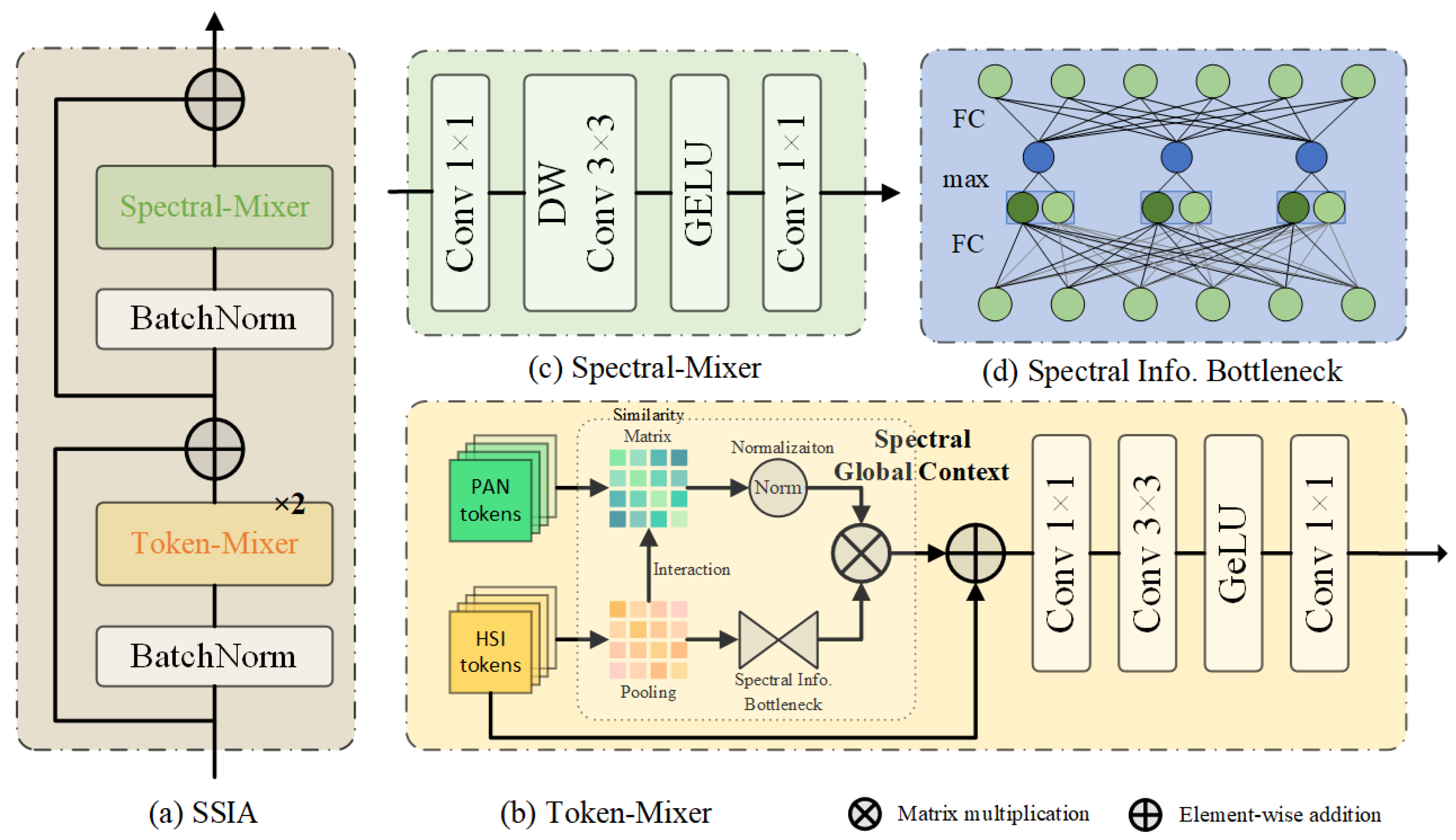
• We design the residual attention-interactive module to simultaneously capture the short- and long-range dependencies of HSI and PAN, in which an specialized spectral-spatial interactive attention is proposed to globally interact and fuse the spectral and spatial features.
• Comprehensive experiments on three public datasets quantitatively and qualitatively demonstrate the effectiveness and superiority of the proposed method. We clearly exhibit the global attention behaviors of our interactive attention through visualization of the heat maps.

2. Related Work

As a pivotal component within Transformer, the self-attention mechanism effectively captures the long-range dependencies of given input features $X\in {\mathbb{R}}^{n\times d}$. n and d represent the patch number and hidden dimension, respectively.

$$y_i=\sum _{j=1}^{n}w\left(q_j,k_j\right)v_j$$

(1)

$$s.t.,w\left(q_j,k_j\right)=softmax\left(q_i^T{k}_j\right)=\frac{exp\left(q_i^T{k}_j\right)}{{\sum }_{l=1}^{n}exp\left(q_i^T{k}_l\right)}$$

(2)

where, $q_i=W_q{x}_i$, $k_i=W_k{x}_i$, and $v_i=W_v{x}_i$ are patch embeddings derived from X. i, j, and l index a image patch. For simplicity, we ignore the positional embeddings and dimensional scalar. Equation (2) dynamically aggregates global information of input image according to each query patch.

Contrary to wide belief that Query, Key, and Value are all necessary, experiments in [35] reveal a Query-irrelevant behavior of self-attention mechanism. Building upon this observation, a variant attention without Query is formulated as follows:

$$y=\sum _{j=1}^{n}w\left(k_j\right)v_j=\sum _{j=1}^n\frac{exp\left(k_j\right)}{{\sum }_{l=1}^{n}exp\left(k_j\right)}=Norm\left(\mathbf{K}\right)\mathbf{V}=gc$$

(3)

where, $Norm(·)$ and $gc\in {\mathbb{R}}^d$ denote normalization operation and global context, respectively. According to the redefinition in Equation (3), the cost of self-attention mechanism is significantly reduced. Furthermore, a simple implementation that directly introduces the global context into local patch can be defined as follows:

$$y_i=\sum _{j\in \omega }{w}_j(x_j+gc)$$

(4)

where, $\omega$ indicates convolutional kernel. Inspired by aforementioned observations, we are encouraged to design a specialized self-attention mechanism for HS pansharpening.

3. Methodology

In this section, we will detailed describe our AIDB-Net as shown in Figure 1, including the Overlapping Patch Embedding Block, Residual Attention-Interactive (Res-AI) Module, and Residual Reconstruction Layer.

3.1. Overlapping Patch Embedding Block

We first introduce the Overlapping Patch Embedding (OEn) block, which is implemented using a convolutional layer followed by batch normalization. In contrast to previous pansharpening models, we design OEn for the purpose of transforming the input HSI and PAN into a sequence of image patch embeddings (tokens) for subsequent attention operation, instead of feature extraction only. Specifically, we employ a HSI Overlapping Patch Embedding (HSI-OEn) block for HSI and a PAN Overlapping Patch Embedding (PAN-OEn) block for PAN, respectively. As shown in Figure 1, PAN-OEn and HSI-OEn are explicitly independent as there are not connections between them. However, they are implicitly related due to the complementary semantics within the PAN and HSI. To broadly spread the information during the tokenization procedure, we intentionally apply an overlapping patch embedding strategy. This approach can facilitate the transmission of the spatial information among adjacent image patches and maintain content consistency between the corresponding tokens from diverse modalities. Moreover, OEn blocks are able to project the HSI and PAN into a cross-modality feature space, achieving alignment of the diverse modality features. Despite its simple structure, OEn is significant for AIDB-Net, connecting both the primary and subsidiary branches.

In details, PAN-OEn is derived from PAN P, as shown in Figure 1. We first partition the PAN P into a sequence of spatially overlapping image patches, each of which is then transformed into a token, encapsulating the original patch information. This transformation is achieved through a stride convolution:

$$P_{EB}=\left\{f\left(p_i\right)\right|i=1,\cdots ,n\},s.t.,n=\frac{1}{4}{(2W-k+1)}^2$$

(5)

where, i indexes each PAN image patch $p_i\in {\mathbb{R}}^{k\times k\times 1}$ in $P\in {\mathbb{R}}^{W\times H\times 1}$, $P_{EB}\in {\mathbb{R}}^{W\times H\times d}$ denotes the feature map of PAN tokens, n is the number of image patches related to the patch size k and the image width W, $f\left(p_i\right)$ represents the transformation function applied to $p_i$.

Similarly, HSI-OEn is applied to HSI as follows:

$$H_{EB}=\left\{f\left(h_i\right)\right|i=1,\cdots ,n\}$$

(6)

where, i indexes each HSI image patch $h_i\in {\mathbb{R}}^{k\times k\times B}$ in $H_{DHP}\in {\mathbb{R}}^{W\times H\times B}$, $H_{EB}\in {\mathbb{R}}^{W\times H\times d}$ denotes the feature map of HSI tokens, $f\left(h_i\right)$ represents the transformation function applied to $h_i$. As shown in Figure 1, we employ DHP [36] algorithm for the purpose of up-sampling the low spatial resolution HSI $H_{LR}\in {\mathbb{R}}^{w\times h\times B}$ into PAN scale, resulting in up-sampled HSI $H_{DHP}$.

3.2. Residual Attention-Interactive Module

As the foundational module of our AIDB-Net, the Residual Attention-Interactive (Res-AI) Module is designed to simultaneously capture the short- and long-range dependencies and effectively fuse the cross-modality features. AS illustrated in Figure 1, the Res-AI module consists of residual learning part for local feature extraction and Spectral-Spatial Interactive Attention (SSIA) part for globally fusing the spectral and spatial features. The capacity of our AIDB-Net is mainly controlled by the number N of sequentially stacked Res-AI modules. Specially, given the number N of Res-AI modules, HSI tokens $H_{EB}$ and PAN tokens $P_{EB}$, we define the primary branch as follows:

$$F_N=f_N(f_{N-1}(\dots f_1(H_{EB},P_{EB})\dots ),P_{EB})$$

(7)

where, $f_N$ represents the function of the primary branch. As illustrated in Figure 1, after passing through all Res-AI modules, the spectral features from the primary have been iteratively interacted with the advanced spatial prior from the subsidiary branch for N times. Consequently, we obtain a highly informative feature representation $F_N$ with both high fidelity spectral and spatial features, which can be utilized to reconstruct the ideal HSI.

3.2.1. Token-Mixer and Spectral-Mixer

As shown in Figure 2a, we construct a transformer-encoder style block in Res-AI module, which consists of Token-Mixer Figure 2b and Spectral-Mixer Figure 2c, along with the residual learning and batch normalization.

In Token-Mixer, we design a interactive attention to abstract the global context by token-global similarity based on the HSI and PAN tokens. Subsequently, the global context will be propagated into each local HSI token in order to combine the global and local information. To fully preserve the spectral features, we introduce the spectral information bottleneck into Token-Mixer, as shown in Figure 2d. Moreover, a series of convolutional layers are employed to further aggregate features at the latter part of the Token-Mixer. In conclusion, we construct a Token-Mixer which is able to globally fuse the cross-modality features and simultaneously model the short- and long-range dependencies.

$$F_{Token}=f_{conv}^{1\times 1}\left(GeLU\left(f_{conv}^{1\times 1}\left(f_{conv}^{3\times 3}(H_{EB}+gc)\right)\right)\right)$$

(8)

where, $F_{Token}$ is a tentatively fused feature, $f_{conv}^{1\times 1}$ and $f_{conv}^{3\times 3}$ represent a point-wise and $3\times 3$ convolution, respectively. $GeLU$ denotes the Gaussian Error Linear Unit [37].

As shown in Figure 2c, the Spectral-Mixer is design to further fuse the polymeric features generated by Token-Mixer.

$$F_N=f_{conv}^{1\times 1}\left(GeLU\left(f_{DWconv}^{3\times 3}\left(f_{conv}^{1\times 1}\left(F_{Token}\right)\right)\right)\right)$$

(9)

where, $f_{DWconv}^{3\times 3}$ denotes a $3\times 3$ depth-size convolution. Note that we set a growth ratio in channel dimension between two contiguous $f_{conv}^{1\times 1}$ layers to fully exploit the relationships among adjacent spectral bands.

3.2.2. Spectral-Spatial Interactive Attention

In this section, we will describe our Spectral-Spatial Interactive Attention (SSIA). The Figure 2b–d demonstrate the detailed structures of the various parts in SSIA. Given the Equation (3), our SSIA is formulated as follows:

$$gc=Norm\left(\mathbf{K}\right)\mathbf{V}=\frac{1}{WH}\sum _{i=1}^n{h}_i^{\prime }$$

(10)

where, $h_i^{\prime }\in {\mathbb{R}}^{k\times k\times d}$ denotes a token in $H_{EB}$. Since Equation (10) solely relies on HSI tokens to construct the global context, we denote it as the spectral global context $gc\in {\mathbb{R}}^d$. Specifically, $gc$ is normalized by average-pooling operation, which is not only for the simplicity but also to ensure each token uniformly aggregates information from its nearby tokens [38].

However, directly integrating the spectral global context defined in Equation (10) with each token in $H_{EB}$ may lead to limited improvement, since that $gc$ will be broadcasted equally for each of them. More importantly, $gc$ lacks the advanced spatial prior from the PAN. To circumvent above problems, we update the spectral global context $gc$ by the token-global similarity calculated from $H_{EB}$ and $P_{EB}$. Specially, given the HSI tokens $H_{EB}$ and PAN tokens $P_{EB}$, we first reshape them into $H_{EB}^{\prime }\in {\mathbb{R}}^{WH\times d}$ and $P_{EB}^{\prime }\in {\mathbb{R}}^{WH\times d}$, respectively. Then the cross-modality token-global similarity $S\in {\mathbb{R}}^{WH}$ is defined as:

$$S={\left(\frac{1}{WH}{H}_{EB}^{\prime }\right)}^T{P}_{EB}^{\prime }$$

(11)

The token-global similarity dynamically calculate the similarity scores of each pixel according to their global cross-modality dependencies, which can be used as guideline to update the spectral characteristics and refine the textural details.

$$g{c}^{\prime }=S^{\prime }gc=(\alpha \frac{S-{\mu }_s}{{\sigma }_s+ϵ}+\beta )gc$$

(12)

where, $S^{\prime }\in {\mathbb{R}}^{WH}$ denotes the normalized S, ${\mu }_s$ and ${\sigma }_s$ are mean and standard deviation, $\alpha$ and $\beta$ are learnable scalars, and $ϵ={10}^{-5}$ maintains numerical stability. By doing so, the updated $g{c}^{\prime }\in {\mathbb{R}}^{WH\times d}$ dynamically aggregates the spatial prior knowledge from the PAN. Then the enhanced global context will be further introduced into the local HSI tokens $H_{EB}$ by Equation (8).

Following the generalization insight of the multi-head self-attention [29], we further extend our interactive attention into multi-group similarity to emphasize more diverse patterns and representation. Specifically, we first divide the spectral global context $gc$, $\frac{1}{WH}{H}_{EB}^{\prime }$, and $P_{EB}^{\prime }$ into G groups along channel dimension. Then, we perform the operation in Equation (12) for each group.

$$g{c}^{\prime }=Concat(S_1^{\prime }g{c}_1,S_2^{\prime }g{c}_2,\dots ,S_G^{\prime }g{c}_G)$$

(13)

The multi-group similarity interactive attention adaptively focuses on pixels of the ground objects according to the similar cross-modality features. The behaviors within each group are complementary. In ablation section, we will verify the globality and diversity of our multi-group similarity interactive attention though quantitative evaluation and visualization.

To further improve the spectral preservation, we apply a spectral information bottleneck to extract the significant spectral characteristics.

$$gc=W_{r}max(W_{1}gc,W_{2}gc)$$

(14)

where, $W_1\in {\mathbb{R}}^{\frac{d}{r}\times d}$, $W_2\in {\mathbb{R}}^{\frac{d}{r}\times d}$, and $W_r\in {\mathbb{R}}^{d\times \frac{d}{r}}$ represent fully connected layer, r is a reduction ratio.

3.3. Residual Reconstruction Layer

After obtained $F_N$, we apply a single convolution as residual reconstruction layer to recover the dimension and reconstruct the residual HSI.

$$H_{Res}=f_{conv}^{3\times 3}\left(F_N\right)=f_{AIDB-Net}\left(H_{DHP},P\right)$$

(15)

where, $H_{Res}$ is the residual HSI and $f_{AIDB-Net}$ denotes the function of our AIDB-Net.

Finally, the fused HSI $H_{Fus}$ can be obtained by summation between $H_{DHP}$ and $H_{Res}$.

$$H_{HR}=H_{DHP}+H_{Res}$$

(16)

3.4. Loss Function

In this paper, we adopt a weighted combinatorial loss function to optimize the proposed method in terms of pixel- and feature-wise. $L_1$ is a pixel-wise loss function which has demonstrated its effectiveness for HS pansharpening in many works.

$$L_1=\frac{1}{CWH}{\parallel H_{Ref}-H_{Fus}\parallel }_1$$

(17)

where, $C,W,H$ the shape of the reference HSI $H_{Ref}$. In addition to $L_1$ loss, we also introduce a feature-wise VGG perceptual loss.

$$L_{vgg}=\frac{1}{C_i{W}_i{H}_i}{\parallel f_i^{vgg}\left(H_{Ref}^{RGB}\right)-f_i^{vgg}\left(H_{Fus}^{RGB}\right)\parallel }_2$$

(18)

where, ${\parallel ·\parallel }_2$ denote $L_2$ norm, $C_i$, $W_i$, $H_i$ represent the shape of feature map $f_i^{vgg}(·)$ at ith layer in VGG19 [39], $H_{Ref}^{RGB}$ and $H_{Fus}^{RGB}$ are synthesized RGB version of $H_{Ref}$ and $H_{HR}$, respectively.

In summary, a weighted combinatorial loss function is defined as follows:

$$L={\lambda }_1{L}_1+{\lambda }_2{L}_{vgg}$$

(19)

where, ${\lambda }_1$ and ${\lambda }_2$ are regularization constants. In this paper, they are set as 1 and 0.1, respectively.

4. Experimental Results

4.1. Experimental Datasets

Three publicly and widely common remote sensing datasets, including Pavia Centre [40], Botswana [41], and Chikusei [42], are selected as experimental datasets to evaluate the performance of our AIDB-Net. We follow the Wald’s protocol [43] to generate PAN, low resolution HSI, and reference HSI for training. The scaling factor is set as 4 for all datasets.

4.1.1. Pavia Centre

The image of Pavia Centre, originally containing 1096 × 1096 pixels and consisting of 115 spectral bands spanning from 430 to 860 nm, was captured by the airborne reflective optics system imaging spectrometer (ROSIS) sensor at a 1.3-m geometric resolution over the City of Pavia, Italy. However, 13 noisy spectral bands and a 381-pixel-wide area with no information were discarded and we intercepted a two-part image with 1096 × 715 × 102 for experimentation. In our experimental design, we used the up-left corner of size 960 × 640 × 102 of the image and partition it into 24 image patches of size 160 × 160 × 102 with no spatially overlap as the reference HSIs. Following the Wald’s protocol [43], we average first 61 spectral bands of the reference HSIs to generate PAN images of size 160 × 160 × 1. In order to generate the low resolution HSIs of size 40 × 40 × 102, we spatially blurred the reference HSIs with Gaussian filter and then down-sampled the results with the scaling factor 4. We randomly select 17 cubic patches (about 70%) for training and the rest 7 cubic patches for testing.

4.1.2. Botswana

The image of Botswana, originally containing 1496 × 256 pixels and consisting of 242 spectral bands spanning from 400 to 2500 nm in 10-nm windows, was captured by the NASA’s Earth Observing 1 (EO-1) satellite at a 30-m geometric resolution over the Okavango Delta, Botswana. However, 97 uncalibrated and noisy spectral bands were removed and we intercepted a image with 1496 × 256 × 145 for experimentation. In our experimental design, we used the up-left corner of size 1200 × 240 × 145 of the image and partition it into 24 image patches of size 120 × 120 × 145 with no spatially overlap as the reference HSIs. Following the Wald’s protocol [43], we average first 31 spectral bands of the reference HSIs to generate PAN images of size 120 × 120 × 1. In order to generate the low resolution HSIs of size 30 × 30 × 145, we spatially blurred the reference HSIs with Gaussian filter and then down-sampled the results with the scaling factor 4. We randomly select 17 cubic patches (about 70%) for training and the rest 7 cubic patches for testing.

4.1.3. Chikusei

The image of Chikusei, originally containing 2517 × 2335 pixels and consisting of 128 spectral bands spanning from 363 to 1018 nm, was captured by the Headwall Hyperspec-VNIR-C imaging sensor at a 2.5-m geometric resolution over the agricultural and urban areas in Chikusei, Japan. There are no noisy spectral bands and blank area need to be discarded. In our experimental design, we used the up-left corner of size 2304 × 2304 × 128 for experiment and partition it into 81 image patches of size 256 × 256 × 128 with no spatially overlap as the reference HSIs. Following the Wald’s protocol [43], we average first 65 spectral bands of the reference HSIs to generate PAN images of size 256 × 256 × 128. In order to generate the low resolution HSIs of size 64 × 64 × 128, we spatially blurred the reference HSIs with Gaussian filter and then down-sampled the results with the scaling factor 4. We randomly select 61 cubic patches (about 75%) for training and the rest 20 cubic patches for testing.

4.2. Quantitative Metrics

In order to quantitatively evaluate the performance of the proposed and competing methods, we select a total of six commonly used pansharpening and super-resolution metrics. Let $x_{fus}$ and $x_{ref}$ denote the fused and reference HSI, respectively.

4.2.1. Cross-Correlation (CC)

CC [44] indicates the spatial correlation between $x_{fus}$ and $x_{ref}$.

$$CC(x_{fus},x_{ref})=\frac{1}{l}\sum _{i=1}^{l}CCS(x_{fus},x_{ref})$$

(20)

$$CCS(A,B)=\frac{{\sum }_{j=1}^n(A_j-{\mu }_A)(B_j-{\mu }_B)}{\sqrt{{\sum }_{j=1}^n{(A_j-{\mu }_A)}^2{(B_j-{\mu }_B)}^2}}$$

(21)

where, l is the number of spectral bands, $\mu$ and n denote the sample mean and the number of pixels, respectively. The optimal CC is 1.0.

4.2.2. Spectral Angle Mapping (SAM)

SAM [44] measures the spectral angle of each pixel between $x_{fus}$ and $x_{ref}$.

$$SAM(x_{fus},x_{ref})=arccos\left(\frac{\langle x_{fus},x_{ref}\rangle }{{\parallel x_{fus}\parallel }_2{\parallel x_{ref}\parallel }_2}\right)$$

(22)

where, $\langle ·,·\rangle$ denote the inner product. The optimal SAM is 0.0, and a smaller value indicates less spectral distortions.

4.2.3. Root-Mean-Squared Error (RMSE)

RMSE [44] represents the difference between $x_{fus}$ and $x_{ref}$.

$$RMSE(x_{fus},x_{ref})=\frac{{\parallel x_{fus}-x_{ref}\parallel }_F}{\sqrt{n\times l}}$$

(23)

where, ${\parallel ·\parallel }_F$ denotes the Frobenius norm. The optimal RMSE is 0.0.

4.2.4. Errur Relative Globale Adimensionnelle Desynthese (ERGAS)

The ERGAS [44] offers a global spectral quality evaluation of $x_{fus}$.

$$ERGAS(x_{fus},x_{ref})=100\frac{1}{{\gamma }^2}\sqrt{\frac{1}{l}\sum _{i=1}^l\left(\frac{RMSE(x_{fus}^i,x_{ref}^i)}{{\mu }_i}\right)}$$

(24)

where, $RMS{E}_i$ represents the RMSE between $x_{fus}$ and $x_{ref}$ in i spectral band, and $\gamma$ is the scaling factor. The optimal ERGAS is 0.0.

4.2.5. Peak Signal to Noise Ratio (PSNR)

PSNR [44] evaluates the spatial quality of each band between $x_{fus}$ and $x_{ref}$.

$$PSNR(x_{fus},x_{ref})=\frac{1}{l}\sum _{i=1}^l\left[10lo{g}_{10}\left(\frac{max\left(x_{ref}^i\right)}{RMSE(x_{fus}^i,x_{ref}^i)}\right)\right]$$

(25)

where, $max\left(x_{ref}^i\right)$ denotes the maximum pixel value in the ith band. The higher the value of PSNR, the better the quality is.

4.2.6. Structural Similarity (SSIM)

SSIM [45] measures the structural similarity index between $x_{fus}$ and $x_{ref}$.

$$SSIM\left(x_{fus},x_{ref}\right)=\frac{\left(2{\mu }_{x_{fus}}{\mu }_{x_{ref}}+C_1\right)\left(2{\sigma }_{x_{fus}{x}_{ref}}+C_2\right)}{\left({\mu }_{x_{fus}}^2+{\mu }_{x_{ref}}^2+C_1\right)\left({\sigma }_{x_{fus}}^2+{\sigma }_{x_{ref}}^2+C_2\right)}$$

(26)

where, ${\sigma }_{x_{fus}{x}_{ref}}$ denotes the covariance between $x_{fus}$ and $x_{ref}$. The optimal value of SSIM is 1.

4.3. Experimental Setup

In this section, we introduce the experimental configurations of the proposed method. We utilize the DHP [23,24,36] algorithm to up-sample the low resolution HSI. All DL-based methods are built upon the Pytorch DL framework. The hyper parameters of our AIDB-Net are presented in

Table 3. The Implementation Details of the Proposed Method.

Hyperparameter	Value
N of Res-AI Modules	3
G of attention groups	8
r of information bottleneck	16
hidden dimension d	64
kernel size	3
batch size	8
optimizer	Adam
epoch	1500
learning rate	${10}^{-3}$
learning scheduler	1000
weight decay	${10}^{-4}$
momentum	0.99

. There are four hyperparameters directly related to our model, which are the kernel size, hidden dimension, reduction ratio of the spectral information bottleneck, attention groups and numbers of the Res-Al modules. We observed that the attention groups have a considerable impact on the model, and we recommend setting it to 8.

4.4. Comparisons

In this section, we compare our AIDB-Net with several classical and advanced HS pansharpening methods, including Principal Component Analysis (PCA) [9], Smoothing Filter-based Intensity Modulation (SFIM) [12], Gram-Schmidt (GS) [10], Gram-Schmidt Adaptive (GSA) [11], Coupled Non-negative Matrix Factorization (CNMF) [16], Modulation Transfer Function with Generalized Laplacian Pyramid (MTF-GLP) [13], PanNet [20], Dual-Branch Detail Extraction Network (DBDENet) [26], Dual Attention Residual Network (DARN), and HyperKite [23]. The experimental results are reported in table and visualization.

4.4.1. Experimental Results on the Pavia Centre Dataset

The average quantitative results of the proposed and competing methods on the Pavia Centre dataset are presented in

Table 4. Average Quantitative Results of the Proposed and Competing HS pansharpening Methods on the Pavia Centre Dataset. The best results are highlighted in bold.

Method	CC	SAM	RMSE $\times {10}^{-2}$	ERGAS	PSNR	SSIM
PCA	0.901	9.38	3.70	6.85	28.51	0.829
SFIM	0.935	7.59	3.25	6.11	29.15	0.866
GS	0.963	7.57	2.81	5.29	30.46	0.880
GSA	0.948	7.79	2.88	5.37	30.37	0.880
CNMF	0.840	7.72	4.88	8.95	25.55	0.666
MTF-GLP	0.942	8.06	3.01	5.64	29.88	0.881
PanNet	0.966	6.58	1.95	4.02	32.07	0.916
DBDENet	0.970	6.90	1.81	4.04	32.42	0.918
DARN	0.973	6.40	1.60	3.80	34.19	0.927
HyperKite	0.975	6.36	1.59	3.77	34.28	0.930
Ours	0.982	5.13	1.35	2.50	36.09	0.944
Optimal	1	0	0	0	$+\infty$	1

. As shown in the table, our AIDB-Net achieves the highest values of CC, PSNR, and SSIM, and the lowest values of SAM, RMSE, and ERGAS, which demonstrates better spectral preservation and spatial enhancement by our model.

Moreover, we represent the visual results corresponding error images in Figure 3 and Figure 4, respectively, in order to shown the qualitative performance. Compare with the competing pansharpening methods, our AIDB-Net produces more visual pleasant images and induces minimum errors. The quantitative and qualitative results exhibited above firmly verify the effectiveness and superiority of the proposed method.

In order to evaluate the spectral preservation capability of the proposed and competing HS pansharpening methods, Figure 5 represents the spectral reflectance difference value comparison of four randomly selected locations with coordinate (10,23), (29,137), (123,65), and (136,113) on the Pavia Centre dataset 21th image. As shown in Figure 5, the proposed method produces minimum difference value which means our AIDB-Net achieves the best spectral fidelity preservation.

4.4.2. Experimental Results on the Botswana Dataset

On the Botswana dataset, we report the average quantitative results in

Table 5. Average Quantitative Results of the Proposed and Competing HS pansharpening Methods on the Botswana Dataset. The best results are highlighted in bold.

Method	CC	SAM	RMSE $\times {10}^{-2}$	ERGAS	PSNR	SSIM
PCA	0.931	2.58	2.12	2.39	27.85	0.952
SFIM	0.931	2.33	1.89	2.22	28.76	0.953
GS	0.937	2.46	2.01	2.27	28.25	0.955
GSA	0.944	2.22	2.68	1.99	29.91	0.960
CNMF	0.829	2.58	2.84	3.21	24.94	0.863
MTF-GLP	0.936	2.24	1.79	2.13	29.08	0.958
PanNet	0.930	2.06	1.50	2.78	29.41	0.945
DBDENet	0.945	2.14	1.52	2.02	29.94	0.961
DARN	0.954	1.83	1.25	1.93	30.69	0.970
HyperKite	0.955	1.86	1.19	1.97	30.77	0.971
Ours	0.968	1.64	1.04	1.52	31.73	0.979
Optimal	1	0	0	0	$+\infty$	1

. Our AIDB-Net outperforms the other pansharpening methods across all six metrics once again, improving CC by 1.36%, PSNR by 3.11%, and SSIM by 0.82%, reducing SAM 10.3%, RMSE by 12.6%, and ERGAS by 22.8%.

The visualization results and corresponding error images are represented in Figure 6 and Figure 7, respectively. As shown in Figure 6, there are noticeable obscurity and chromatism caused by PCA, GS, and CNMF. Different with the results on Pavia, some traditional pansharpening methods including SFIM, GSA, and MTF-GLP achieve competitive quantitative performance on Botswana. However, their corresponding error images appear much lighter, indicating their poor visual performance.

On the other hand, PanNet, DBDENet, DARN, and HyperKite exhibit slight spectral distortions in certain image parts. Back to our AIDB-net, we can obviously observed that the pansharpened image generated by AIDB-Net is the closest to the ground truth in terms of both color and texture.

Moreover, as shown in Figure 8b, our AIDB-net has achieved the best PSNR scores in most spectral bands. In a summary, our AIDB-Net obtain the best pansharpening performance on the Botswana dataset.

4.4.3. Experimental Results on the Chikusei Dataset

The quantitative and qualitative results on the Chikusei dataset are represented in

Table 6. Average Quantitative Results of the Proposed and Competing HS pansharpening Methods on the Chikusei Dataset. The best results are highlighted in bold.

Method	CC	SAM	RMSE $\times {10}^{-2}$	ERGAS	PSNR	SSIM
PCA	0.778	6.38	3.54	10.61	25.66	0.828
SFIM	0.926	4.05	2.02	7.18	29.58	0.904
GS	0.946	4.01	1.82	6.38	30.53	0.912
GSA	0.937	4.27	1.75	6.88	30.74	0.918
CNMF	0.935	3.99	3.42	8.78	26.12	0.813
MTF-GLP	0.932	4.17	1.93	6.90	29.95	0.914
PanNet	0.946	3.28	1.92	5.55	31.74	0.926
DBDENet	0.957	3.64	1.48	5.22	33.27	0.939
DARN	0.955	3.65	1.44	5.07	33.49	0.935
HyperKite	0.957	3.70	1.41	5.11	33.81	0.941
Ours	0.971	3.05	1.14	4.75	34.57	0.956
Optimal	1	0	0	0	$+\infty$	1

and Figure 9 and Figure 10, respectively. As shown in Table 6, almost all competing methods, except PCA, yield satisfied performance aspects of quantitative assessments, particularly our AIDB-Net achieves the best.

We visualize the error images in Figure 10. It’s obviously see that the proposed method presents less error. To further shown the perceptual quality, Figure 9 exhibits the reconstructed images. As shown in Figure 9, almost all traditional methods suffer from blurry effects. While for PanNet, DBDENet, DARN, and HyperKite show relatively better quality, but not enough. Our AIDB-Net generates pansharpened images with both high spectral and spatial quality.

4.5. The Impact of Dual-Branch Learning Strategy

The dual-branch learning strategy is crucial for our AIDB-Net, as it not only provides aligned HSI and PAN tokens but also relates to our interactive attention. To choose the most suitable learning strategy, we have totally tested three different implementations, which are described as follows:

• HSI-PAN: As illustrated in Figure 11a, the HSI and PAN are initially tokenized using HSI-OEn and PAN-OEn, respectively. Subsequently, our SSIA receives HSI tokens (spectral information) as primary feature and PAN tokens (spatial information) as auxiliary feature to calculate the token similarity scores.
• PAN-HSI: Contrary to HSI-PAN in Figure 11a, we select the PAN and HSI tokens as primary and auxiliary features, respectively, as shown in Figure 11b. Consequently, the fused feature is derived from the PAN tokens instead of HSI tokens.
• HSI+PAN: Following the previous DL-based methods, we have also explored the feasibility of concatenation as a learning strategy for our model. As depicted in Figure 11c, we first concatenate the HSI and PAN along channel dimension. Then, we utilize a single embedding block to generate hybrid tokens for latter attention operation.

For simplicity, we denote these three different learning strategies as HSI-PAN, PAN-HSI, and HSI+PAN, respectively. It’s important to note that their parameters and computational complexity are totally identical, thus the quantitative results are objective. As shown in

Table 7. Average Quantitative Results of Different Learning Strategies on the Pavia Centre Dataset. The best results are highlighted in bold.

Learning Strategy	CC	SAM	RMSE $\times {10}^{-2}$	ERGAS	PSNR	SSIM
(a) HSI-PAN	0.982	5.13	1.35	2.50	36.09	0.944
(b) PAN-HSI	0.932	6.45	2.89	4.21	30.61	0.883
(c) HSI+PAN	0.929	6.49	2.99	4.37	30.23	0.875
Optimal	1	0	0	0	$+\infty$	1

, both PAN-HSI and HSI+PAN exhibit a relatively low pansharpening performance across six metrics, suggesting that they are improper for our AIDB-Net. The learning strategy of HSI-PAN achieves the best performance over all evaluation measurements which firmly verify its effectiveness. Meanwhile, our ablation study also demonstrates that the concatenation of a single spectral band PAN with hundreds of spectral bands HSI is inferior in fusing the spectral and spatial information.

4.6. The Impact of Number N

The size of our AIDB-Net is mainly controlled by the number N of Res-AI modules. To identify the optimal N, we test the affect of number N ranging from 1 to 6. The quantitative results in

Table 8. Average Quantitative Results of Different Number N on the Pavia Centre dataset. The best results are highlighted in bold.

N	CC	SAM	RMSE $\times {10}^{-2}$	ERGAS	PSNR	SSIM
1	0.974	6.02	1.71	2.89	34.93	0.934
2	0.976	5.58	1.49	2.68	35.70	0.937
3	0.982	5.13	1.35	2.50	36.09	0.944
4	0.976	5.65	1.47	2.55	35.79	0.941
5	0.977	5.74	1.55	2.63	35.85	0.939
6	0.976	5.72	1.56	2.66	35.78	0.939
Optimal	1	0	0	0	$+\infty$	1

show that the pansharpening performance firstly increases until $N=3$ and then begins to decrease. Consequently, we set 3 as the optimal choice.

4.7. The Impact of Number G

As previously stated, we have intentionally designed a multi-group similarity interactive attention for the proposed methods. Each group of our interactive attention are complementary and can adaptively emphasize the pixels according to the diverse cross-modality features. In this section, we design a series of ablation experiments in order to demonstrate the effectiveness, adaptability, and diversity of our multi-group similarity interactive attention and reveal its attention behaviors. As shown in

Table 9. Average Quantitative Results of Different Number G on the Pavia Centre dataset. The best results are highlighted in bold.

G	CC	SAM	RMSE $\times {10}^{-2}$	ERGAS	PSNR	SSIM
1	0.975	5.98	1.63	3.51	35.46	0.931
2	0.977	5.67	1.51	3.13	35.73	0.935
4	0.978	5.51	1.40	2.79	35.85	0.937
8	0.982	5.13	1.35	2.50	36.09	0.944
16	0.976	5.72	1.56	2.66	35.99	0.935
Optimal	1	0	0	0	$+\infty$	1

, we first investigate the quantitative performance impact of the group number G from 1 to 16. The value of G should be a factor of the model’s hidden dimension. We can obviously see that increasing the group number G leads to a remarkable improvement on the spectral and spatial quantitative metrics, which firmly demonstrate the effectiveness of our interactive attention. Following the table, We set $G=8$ as the optimal choice.

As shown in Figure 12, we visualize the heat maps within the first Token-Mixer to visually exhibit the attention behaviors.

It is important to note that different colors in the heat map represent different attention degrees, with yellow indicating high attention and blue indicating low. Pixels with similar colors are considered related in the cross-modality feature space by the interactive attention, while pixels with opposite colors are deemed irrelevant. As depicted in Figure 12, each group of the multi-group similarity adaptively emphasize ground objects based on the similarity scores of the global cross-modality features. The attention behaviors of each group is different, which straightforward demonstrate the adaptability and diversity of the multi-group similarity. Although the heat maps of the 1st, 3rd–5th, and 7th groups appear somewhat similar overall, they differ in details. This observation illustrates that each group in the multi-group similarity is complementary and cooperative to others, ultimately resulting in the restoration of textural details and preservation of spectral characteristics.

4.8. Parameters

To evaluate the computational complexity and time cost of our AIDB-Net,

Table 10. Comparisons of the Parameters, FLOPs, Epochs, and Inference Time on the Pavia Centre Dataset.

Model	Parameters	FLOPs	Epoch	Inference Time
PanNet	0.675 M	15.45G	1000	0.138 s
DBDENet	5.667 M	48.53G	1500	0.422 s
DARN	0.416 M	10.58G	1000	0.131 s
HyperKite	0.524 M	341.58G	2000	2.720 s
Ours	0.563 M	14.31G	1500	0.184 s

provide the parameters, FLOPs, convergence speed (epoch), and inference time. All tesinng experiments are conducted on Intel Core i7-11800H CPU and NVDIA RTX 3060 Laptop GPU (6 GB). As shown in the table, on the one hand, our AIDB-Net has comparable parameters and FLOPs compared to PanNet and DARN, far less than DBDENet and HyperKite. On the other hand, the convergence speed (epochs) and inference time of our AIDB-net is slightly longer than PanNet and DARN, faster than DBDENet and HyperKite. Considering the pansharpening performance improved by our AIDB-Net, the memory and time cost are acceptable.

5. Limitation and Discussion

Omission of Small-Scale Ground Objects

In the fused HSI generated by our AIDB-Net, we have observed problems of the reduction or omission of small-scale ground objects. Furthermore, we find the same issues in other HS pansharpening models as well. That is caused by the inadequate feature representation capability of small-scale ground objects of the model. Within the remote sensing semantic segmentation community, we notice that some researchers pay attention to the extraction of small-scale features to alleviate the above problems. In paper [46], the authors design feature compression module to broadly aggregate features and structural information of small-scale objects by expanding the receptive field of the convolution, thereby improving the classification accuracy of the model. Considering that there are maybe a large number of small-scale objects within the source HSI and PAN, these detailed information should not be reduced or lost within the fused HSI. Therefore, we are encouraged to design a specialized small-scale component for our AIDB-Net to reduce the loss of detailed information and condense small-scale features.

6. Conclusions

In this paper, we are committed to capturing the global cross-modality dependencies between the hyperspectral and panchromatic images to improve the pansharpening performance. We propose an Attention-Interactive Dual-Branch Convolutional Neural Network (AIDB-Net), which purely consists of convolutional layers and firmly inherits the merits of both convolution and self-attention, such as modeling of short- and long-range dependencies. Specially, we first apply a simple and efficient component as tokens generator, features extractor and aligner to process the diverse modality images. Then, a novel spectral-spatial interactive attention is proposed to globally and directly interact and fuse the spectral and spatial features. Consequently, benefit from integration of local and global information, our AIDB-Net achieves the best pansharpening performance. However, the proposed method has shortcomings in feature extraction of small-scale ground objects, which may results reduced textural details and desaturated color over small-scale targets. We will further extend and deepening our study to overcome this limitation.

References

1. Sun, L.; Fang, Y.; Chen, Y.; Huang, W.; Wu, Z.; Jeon, B. Multi-Structure KELM With Attention Fusion Strategy for Hyperspectral Image Classification. IEEE Trans. Geosci. Remote Sens. 2022, 60, 5539217. [Google Scholar] [CrossRef]
2. Sun, L.; Song, X.; Guo, H.; Zhao, G.; Wang, J. Patch-wise semantic segmentation for hyperspectral images via a cubic capsule network with emap features. Remote Sens. 2021, 13, 3497. [Google Scholar] [CrossRef]
3. Sun, L.; Cao, Q.; Chen, Y.; Zheng, Y.; Wu, Z. Mixed Noise Removal for Hyperspectral Images Based on Global Tensor Low-Rankness and Nonlocal SVD-Aided Group Sparsity. IEEE Trans. Geosci. Remote Sens. 2023, 61, 5506617. [Google Scholar] [CrossRef]
4. Sun, L.; Chen, Y.; Li, B. SISLU-Net: Spatial Information-Assisted Spectral Information Learning Unmixing Network for Hyperspectral Images. Remote Sens. 2023, 15, 817. [Google Scholar] [CrossRef]
5. Wang, J.; Shao, Z.; Huang, X.; Lu, T.; Zhang, R. A Dual-Path Fusion Network for Pan-Sharpening. IEEE Trans. Geosci. Remote Sens. 2022, 60, 5403214. [Google Scholar] [CrossRef]
6. Liu, Y.; Hu, J.; Kang, X.; Luo, J.; Fan, S. Interactformer: Interactive Transformer and CNN for Hyperspectral Image Super-Resolution. IEEE Trans. Geosci. Remote Sens. 2022, 60, 5531715. [Google Scholar] [CrossRef]
7. Tu, T.M.; Su, S.C.; Shyu, H.C.; Huang, P.S. A new look at IHS-like image fusion methods. Inf. Fusion 2001, 2, 177–186. [Google Scholar] [CrossRef]
8. Vivone, G.; Alparone, L.; Chanussot, J.; Dalla Mura, M.; Garzelli, A.; Licciardi, G.A.; Restaino, R.; Wald, L. A Critical Comparison Among Pansharpening Algorithms. IEEE Trans. Geosci. Remote Sens. 2015, 53, 2565–2586. [Google Scholar] [CrossRef]
9. Kwarteng, P.; Chavez, A. Extracting spectral contrast in Landsat Thematic Mapper image data using selective principal component analysis. Photogramm. Eng. Remote Sens. 1989, 55, 339–348. [Google Scholar]
10. Laben, C.A.; Brower, B.V. Process for Enhancing the Spatial Resolution of Multispectral Imagery Using Pan-Sharpening. US Patent 6,011,875, 4 January 2000. [Google Scholar]
11. Aiazzi, B.; Baronti, S.; Selva, M. Improving Component Substitution Pansharpening Through Multivariate Regression of MS +Pan Data. IEEE Trans. Geosci. Remote Sens. 2007, 45, 3230–3239. [Google Scholar] [CrossRef]
12. Liu, J. Smoothing filter-based intensity modulation: A spectral preserve image fusion technique for improving spatial details. Int. J. Remote Sens. 2000, 21, 3461–3472. [Google Scholar] [CrossRef]
13. Aiazzi, B.; Alparone, L.; Baronti, S.; Garzelli, A. Context-driven fusion of high spatial and spectral resolution images based on oversampled multiresolution analysis. IEEE Trans. Geosci. Remote Sens. 2002, 40, 2300–2312. [Google Scholar] [CrossRef]
14. Aiazzi, B.; Alparone, L.; Baronti, S.; Garzelli, A.; Selva, M. MTF-tailored multiscale fusion of high-resolution MS and Pan imagery. Photogramm. Eng. Remote Sens. 2006, 72, 591–596. [Google Scholar] [CrossRef]
15. Liao, W.; Huang, X.; Van Coillie, F.; Gautama, S.; Pižurica, A.; Philips, W.; Liu, H.; Zhu, T.; Shimoni, M.; Moser, G.; et al. Processing of Multiresolution Thermal Hyperspectral and Digital Color Data: Outcome of the 2014 IEEE GRSS Data Fusion Contest. IEEE J. Sel. Top. Appl. Earth Obs. Remote Sens. 2015, 8, 2984–2996. [Google Scholar] [CrossRef]
16. Yokoya, N.; Yairi, T.; Iwasaki, A. Coupled Nonnegative Matrix Factorization Unmixing for Hyperspectral and Multispectral Data Fusion. IEEE Trans. Geosci. Remote Sens. 2012, 50, 528–537. [Google Scholar] [CrossRef]
17. Simões, M.; Bioucas-Dias, J.; Almeida, L.B.; Chanussot, J. A Convex Formulation for Hyperspectral Image Superresolution via Subspace-Based Regularization. IEEE Trans. Geosci. Remote Sens. 2015, 53, 3373–3388. [Google Scholar] [CrossRef]
18. Wei, Q.; Dobigeon, N.; Tourneret, J.Y. Bayesian Fusion of Multi-Band Images. IEEE J. Sel. Top. Signal Process. 2015, 9, 1117–1127. [Google Scholar] [CrossRef]
19. Masi, G.; Cozzolino, D.; Verdoliva, L.; Scarpa, G. Pansharpening by convolutional neural networks. Remote Sens. 2016, 8, 594. [Google Scholar] [CrossRef]
20. Yang, J.; Fu, X.; Hu, Y.; Huang, Y.; Ding, X.; Paisley, J. PanNet: A Deep Network Architecture for Pan-Sharpening. In Proceedings of the 2017 IEEE International Conference on Computer Vision (ICCV), Venice, Italy, 22–29 October 2017; pp. 1753–1761. [Google Scholar] [CrossRef]
21. Wei, Y.; Yuan, Q.; Shen, H.; Zhang, L. Boosting the Accuracy of Multispectral Image Pansharpening by Learning a Deep Residual Network. IEEE Geosci. Remote Sens. Lett. 2017, 14, 1795–1799. [Google Scholar] [CrossRef]
22. Peng, J.; Liu, L.; Wang, J.; Zhang, E.; Zhu, X.; Zhang, Y.; Feng, J.; Jiao, L. PSMD-Net: A Novel Pan-Sharpening Method Based on a Multiscale Dense Network. IEEE Trans. Geosci. Remote Sens. 2021, 59, 4957–4971. [Google Scholar] [CrossRef]
23. Bandara, W.G.C.; Valanarasu, J.M.J.; Patel, V.M. Hyperspectral Pansharpening Based on Improved Deep Image Prior and Residual Reconstruction. IEEE Trans. Geosci. Remote Sens. 2022, 60, 5520816. [Google Scholar] [CrossRef]
24. Zheng, Y.; Li, J.; Li, Y.; Guo, J.; Wu, X.; Chanussot, J. Hyperspectral Pansharpening Using Deep Prior and Dual Attention Residual Network. IEEE Trans. Geosci. Remote Sens. 2020, 58, 8059–8076. [Google Scholar] [CrossRef]
25. He, L.; Zhu, J.; Li, J.; Plaza, A.; Chanussot, J.; Li, B. HyperPNN: Hyperspectral Pansharpening via Spectrally Predictive Convolutional Neural Networks. IEEE J. Sel. Top. Appl. Earth Obs. Remote Sens. 2019, 12, 3092–3100. [Google Scholar] [CrossRef]
26. Qu, J.; Hou, S.; Dong, W.; Xiao, S.; Du, Q.; Li, Y. A dual-branch detail extraction network for hyperspectral pansharpening. IEEE Trans. Geosci. Remote Sens. 2021, 60, 1–13. [Google Scholar] [CrossRef]
27. Zheng, Y.; Li, J.; Li, Y.; Guo, J.; Wu, X.; Shi, Y.; Chanussot, J. Edge-Conditioned Feature Transform Network for Hyperspectral and Multispectral Image Fusion. IEEE Trans. Geosci. Remote Sens. 2022, 60, 5513315. [Google Scholar] [CrossRef]
28. Meng, X.; Wang, N.; Shao, F.; Li, S. Vision Transformer for Pansharpening. IEEE Trans. Geosci. Remote Sens. 2022, 60, 5409011. [Google Scholar] [CrossRef]
29. Dosovitskiy, A.; Beyer, L.; Kolesnikov, A.; Weissenborn, D.; Zhai, X.; Unterthiner, T.; Dehghani, M.; Minderer, M.; Heigold, G.; Gelly, S.; et al. An image is worth 16 × 16 words: Transformers for image recognition at scale. arXiv 2020, arXiv:2010.11929. [Google Scholar]
30. Bandara, W.G.C.; Patel, V.M. HyperTransformer: A Textural and Spectral Feature Fusion Transformer for Pansharpening. In Proceedings of the 2022 IEEE/CVF Conference on Computer Vision and Pattern Recognition (CVPR), New Orleans, LA, USA, 18–24 June 2022; pp. 1757–1767. [Google Scholar] [CrossRef]
31. Hu, J.F.; Huang, T.Z.; Deng, L.J.; Dou, H.X.; Hong, D.; Vivone, G. Fusformer: A Transformer-Based Fusion Network for Hyperspectral Image Super-Resolution. IEEE Geosci. Remote Sens. Lett. 2022, 19, 6012305. [Google Scholar] [CrossRef]
32. Zhou, H.; Liu, Q.; Wang, Y. PanFormer: A Transformer Based Model for Pan-Sharpening. In Proceedings of the 2022 IEEE International Conference on Multimedia and Expo (ICME), Taipei, Taiwan, 18–22 July 2022; pp. 1–6. [Google Scholar] [CrossRef]
33. Wu, H.; Xiao, B.; Codella, N.; Liu, M.; Dai, X.; Yuan, L.; Zhang, L. CvT: Introducing Convolutions to Vision Transformers. In Proceedings of the 2021 IEEE/CVF International Conference on Computer Vision (ICCV), Montreal, BC, Canada, 11–17 October 2021; pp. 22–31. [Google Scholar] [CrossRef]
34. Pan, X.; Ge, C.; Lu, R.; Song, S.; Chen, G.; Huang, Z.; Huang, G. On the Integration of Self-Attention and Convolution. In Proceedings of the 2022 IEEE/CVF Conference on Computer Vision and Pattern Recognition (CVPR), New Orleans, LA, USA, 18–24 June 2022; pp. 805–815. [Google Scholar] [CrossRef]
35. Ma, X.; Wang, H.; Qin, C.; Li, K.; Zhao, X.; Fu, J.; Fu, Y. A Close Look at Spatial Modeling: From Attention to Convolution. arXiv 2022, arXiv:2212.12552. [Google Scholar]
36. Sidorov, O.; Yngve Hardeberg, J. Deep hyperspectral prior: Single-image denoising, inpainting, super-resolution. In Proceedings of the IEEE/CVF International Conference on Computer Vision Workshops, Seoul, Republic of Korea, 27–28 October 2019; pp. 3844–3851. [Google Scholar]
37. Hendrycks, D.; Gimpel, K. Gaussian error linear units (gelus). arXiv 2016, arXiv:1606.08415. [Google Scholar]
38. Yu, W.; Luo, M.; Zhou, P.; Si, C.; Zhou, Y.; Wang, X.; Feng, J.; Yan, S. MetaFormer is Actually What You Need for Vision. In Proceedings of the 2022 IEEE/CVF Conference on Computer Vision and Pattern Recognition (CVPR), New Orleans, LA, USA, 18–24 June 2022; pp. 10809–10819. [Google Scholar] [CrossRef]
39. Simonyan, K.; Zisserman, A. Very deep convolutional networks for large-scale image recognition. arXiv 2014, arXiv:1409.1556. [Google Scholar]
40. Plaza, A.; Benediktsson, J.A.; Boardman, J.W.; Brazile, J.; Bruzzone, L.; Camps-Valls, G.; Chanussot, J.; Fauvel, M.; Gamba, P.; Gualtieri, A.; et al. Recent advances in techniques for hyperspectral image processing. Remote Sens. Environ. 2009, 113, S110–S122. [Google Scholar] [CrossRef]
41. Ungar, S.; Pearlman, J.; Mendenhall, J.; Reuter, D. Overview of the Earth Observing One (EO-1) mission. IEEE Trans. Geosci. Remote Sens. 2003, 41, 1149–1159. [Google Scholar] [CrossRef]
42. Yokoya, N.; Iwasaki, A. Airborne Hyperspectral Data over Chikusei; Tech. Rep. SAL-2016-05-27; Space Application Laboratory, the University of Tokyo: Tokyo, Japan, 2016; Volume 5, p. 5. [Google Scholar]
43. Zeng, Y.; Huang, W.; Liu, M.; Zhang, H.; Zou, B. Fusion of satellite images in urban area: Assessing the quality of resulting images. In Proceedings of the 2010 18th International Conference on Geoinformatics, Beijing, China, 18–20 June 2010; pp. 1–4. [Google Scholar] [CrossRef]
44. Loncan, L.; de Almeida, L.B.; Bioucas-Dias, J.M.; Briottet, X.; Chanussot, J.; Dobigeon, N.; Fabre, S.; Liao, W.; Licciardi, G.A.; Simões, M.; et al. Hyperspectral Pansharpening: A Review. IEEE Geosci. Remote Sens. Mag. 2015, 3, 27–46. [Google Scholar] [CrossRef]
45. Wang, Z.; Bovik, A.C.; Sheikh, H.R.; Simoncelli, E.P. Image quality assessment: From error visibility to structural similarity. IEEE Trans. Geosci. Remote Sens. 2004, 13, 600–612. [Google Scholar] [CrossRef]
46. He, X.; Zhou, Y.; Zhao, J.; Zhang, D.; Yao, R.; Xue, Y. Swin transformer embedding UNet for remote sensing image semantic segmentation. IEEE Trans. Geosci. Remote Sens. 2022, 60, 1–15. [Google Scholar] [CrossRef]
Figure 1. The overall architecture of our AIDB-Net adopts a dual-branch learning strategy. Specially, the HSI and PANs are first tokenized by the Overlapping Patch Embedding Blocks within the primary and subsidiary branches, respectively. Then, HSI and PAN features (tokens) are fused through the Spectral-Spatial Interactive Attention within the Residual Attention-Interactive Module, executed step by step. Finally, a convolutional layer, namely Residual Reconstruction Layer, is applied to recover and reconstruct the residual HSI. It’s note that the deep hyperspectral prior is utilized to provide suitable size HSI as input.
Remotesensing 16 01044 g001
Figure 2. The detailed structure of the Token-Mixer (b) and Spectral-Mixer (c). We repeat the operations in Token-Mixer in twice for better generation. Additionally, the Spectral Information Bottleneck (d) is introduced to extract the significant spectral characteristics.
Remotesensing 16 01044 g002
Figure 3. Visual results on the Pavia Centre dataset. (a) Reference. (b) PCA. (c) SFIM. (d) GS. (e) GSA. (f) CNMF. (g) MTF-GLP. (h) PanNet. (i) DBDENet. (j) DARN. (k) HyperKite. (l) AIDB-Net (Ours).
Remotesensing 16 01044 g003
Figure 4. The corresponding mean absolute error images on the Pavia Centre dataset. (a) Reference. (b) PCA. (c) SFIM. (d) GS. (e) GSA. (f) CNMF. (g) MTF-GLP. (h) PanNet. (i) DBDENet. (j) DARN. (k) HyperKite. (l) AIDB-Net (Ours).
Remotesensing 16 01044 g004
Figure 5. Comparison of spectral reflectance difference values of four randomly selected locations in Figure 3. (a) Pixel (10,23). (b) Pixel (29,137). (c) Pixel(123,65). (d) Pixel (136,113).
Remotesensing 16 01044 g005
Figure 6. Visual results on the Botswana dataset. (a) Reference. (b) PCA. (c) SFIM. (d) GS. (e) GSA. (f) CNMF. (g) MTF-GLP. (h) PanNet. (i) DBDENet. (j) DARN. (k) HyperKite. (l) AIDB-Net (Ours).
Remotesensing 16 01044 g006
Figure 7. The corresponding mean absolute error images on the Botswana dataset. (a) Reference. (b) PCA. (c) SFIM. (d) GS. (e) GSA. (f) CNMF. (g) MTF-GLP. (h) PanNet. (i) DBDENet. (j) DARN. (k) HyperKite. (l) AIDB-Net (Ours).
Remotesensing 16 01044 g007
Figure 8. PSNR as a function of spectral band. (a) Pavia Centre dataset. (b) Botswana dataset. (c) Chikusei dataset.
Remotesensing 16 01044 g008
Figure 9. Visual results on the Chikusei dataset. (a) Reference. (b) PCA. (c) SFIM. (d) GS. (e) GSA. (f) CNMF. (g) MTF-GLP. (h) PanNet. (i) DBDENet. (j) DARN. (k) HyperKite. (l) AIDB-Net (Ours).
Remotesensing 16 01044 g009
Figure 10. The corresponding mean absolute error images on the Chikusei dataset. (a) Reference. (b) PCA. (c) SFIM. (d) GS. (e) GSA. (f) CNMF. (g) MTF-GLP. (h) PanNet. (i) DBDENet. (j) DARN. (k) HyperKite. (l) AIDB-Net (Ours).
Remotesensing 16 01044 g010
Figure 11. Three different learning strategies. (a) HSI-PAN. (b) PAN-HSI. (c) HSI+PAN.
Remotesensing 16 01044 g011
Figure 12. Visualization of the multi-group similarity interactive attention, when G = 8 .
Remotesensing 16 01044 g012