Article

Analysing the Relationship between Spatial Resolution, Sharpness and Signal-to-Noise Ratio of Very High Resolution Satellite Imagery Using an Automatic Edge Method

1
School of Aerospace Engineering, Sapienza University of Rome, 00138 Rome, Italy
2
Serco Italia SpA, 00044 Frascati, Italy
3
CIMA Research Foundation, 17100 Savona, Italy
4
European Space Agency (ESA), 00044 Frascati, Italy
*
Author to whom correspondence should be addressed.
Remote Sens. 2024, 16(6), 1041; https://doi.org/10.3390/rs16061041
Submission received: 8 February 2024 / Revised: 12 March 2024 / Accepted: 13 March 2024 / Published: 15 March 2024
(This article belongs to the Special Issue Remote Sensing: 15th Anniversary)

Abstract

:
Assessing the performance of optical imaging systems is crucial to evaluate their capability to satisfy the product requirements for an Earth Observation (EO) mission. In particular, the evaluation of image quality is undoubtedly one of the most important, critical and problematic aspects of remote sensing. It involves not only pre-flight analyses, but also continuous monitoring throughout the operational lifetime of the observing system. The Ground Sampling Distance (GSD) of the imaging system is often the only parameter used to quantify its spatial resolution, i.e., its capability to resolve objects on the ground. In practice, this feature is also heavily influenced by other image quality parameters such as the image sharpness and Signal-to-Noise Ratio (SNR). However, these last two aspects are often analysed separately, using unrelated methodologies, complicating the image quality assessment and posing standardisation issues. To this end, we expanded the features of our Automatic Edge Method (AEM), which was originally developed to simplify and automate the estimate of sharpness metrics, to also extract the image SNR. In this paper we applied the AEM to a wide range of optical satellite images characterised by different GSD and Pixel Size (PS) with the objective to explore the nature of the relationship between the components of overall image quality (image sharpness, SNR) and product geometric resampling (expressed in terms of GSD/PS ratio). Our main objective is to quantify how the sharpness and the radiometric quality of an image product are affected by different product geometric resampling strategies, i.e., by distributing imagery with a PS larger or smaller than the GSD of the imaging system. The AEM allowed us to explore this relationship by relying on a vast amount of data points, which provide a robust statistical significance to the results expressed in terms of sharpness metrics and SNR means. The results indicate the existence of a direct relationship between the product geometric resampling and the overall image quality, and also highlight a good degree of correlation between the image sharpness and SNR.

1. Introduction

The criteria used to evaluate the quality of spaceborne imagery are strictly related to the application for which the acquisition system was originally designed [1]. For instance, weather satellites must observe very large-scale, complex phenomena, which benefit from high radiometric fidelity. On the other hand, imaging systems developed to observe urban environments will favour very high spatial resolutions in order to provide the level of detail needed to detect small targets.
Nevertheless, a complete description of the quality of a spaceborne acquisition system can be given in terms of temporal resolution, spectral resolution, radiometric resolution and spatial resolution [2,3]. While the general concept of satellite image quality in its broadest sense depends on all these factors [4], in this paper we focus specifically on its declination in the context of high-resolution optical imaging systems [5]. Given the variety of perspectives and interpretations in the related literature, which often lead to different definitions of the same concepts and metrics, it is necessary to clarify the terminology used in this paper and the specific meaning we assign to “image quality” in order to avoid confusion. To this end, the long-lasting open issue related to the definition of the concept of spatial resolution and to the identification of a standardised metric to quantify it [2,3,6] serves as an exemplifying example.
These issues are further exacerbated by the fact that some quality metrics can be used both at the sensor level, i.e., to characterise the quality of the sensor per se, and at the image product level, i.e., to characterise the quality of a specific product resulting from the application of a processing pipeline to an image acquired by a sensor. Even when considering only the image product level, as we will do in this paper, it should be noted that the values of the quality metrics may and will vary according to the specific processing level of the image product being analysed. For a comprehensive description of these topics, the reader is invited to refer to [7]. In particular, even when restricting the field to the image-level metrics, the difficulty in comparing results obtained using different methodologies is well known, hence the need for a standardised procedure [2,4,8,9,10].
Hereinafter, we will refer to the concept of “overall image quality” as it was defined in [4], i.e., as the capability of discriminating ground targets in an individual band of a specific product acquired by an optical sensor. This capability is determined by the sensor spatial resolution and by its performance in terms of sharpness and radiometric quality. The temporal and spectral components are not included in this definition, since we focus on the quality of an individual band of a specific image.
This definition has the added benefit of not being limited to spatial imagery, but may be applied to any type of optical imagery. The AEM and its predecessor have been used to analyse aerial imagery [11] and for general-purpose high-resolution image data [12].

1.1. The Concepts of Spatial Resolution and Image Sharpness

The spatial resolution of an optical imaging system is probably the most misleading and confusing factor related to the quality of spaceborne imagery, partially because of the wide variety of metrics used to measure it depending on the context [3]. From a manufacturer perspective, the spatial resolution is often described in terms of the Instantaneous Field Of View (IFOV), which is the solid angle subtended by a single detector element around its own optical axis. However, the objective of an end-user is to extract useful information from the image, and consequently the definition of spatial resolution from a user viewpoint is related to the size of the smallest physical object that can be identified [3]. Consequently, the spatial resolution of the sensor is sometimes described solely in terms of its GSD, which represents the distance on the ground between two consecutive sensor element footprints. However, it is well known that this quantity alone is not sufficient to determine the capability of the system to discriminate objects on the ground, since objects with a characteristic size smaller than the GSD can still be reliably identified if they are sufficiently contrasted with the background [1,7]. The GSD is therefore related to the characteristics of the imaging system and to the observation geometry, and should not be confused with the PS, which is a characteristic of the image product: before being distributed, images undergo a series of post-processing procedures and are resampled to a certain PS, which usually is larger than the GSD. Image products will undergo different degrees of post-processing (e.g., geometric and atmospheric correction, resampling, etc.) depending on the processing level, and consequently, GSD and PS can (and usually will) be different. Their relationship, which in this paper will be quantified by means of the GSD/PS ratio, has an impact on the image quality, which we will analyse in the following sections.
While at a first glance it may appear intuitive, in practice it is quite difficult to define precisely what a “sharp” image is. For this reason, it is not uncommon to see image sharpness defined by contrast, i.e., as the opposite of “blurriness” [4,13], which is a more familiar concept. In fact, it is the other way around: it is blurriness, i.e., lack of clarity, which is defined as the opposite of sharpness, which is the quality of an image of being clear. However, this would lead us to think that the sharper the image, the more details one can extract, and thus the higher the quality. This is not true, as an excessively sharp image can show the opposite effect of blurriness (i.e., “aliasing”) which happens when a scene with a high frequency content is sampled at an insufficient frequency, resulting in a “jagged” appearance and in the presence of non-existent lines or patterns [13,14]. Indeed, sharpness is not a binary condition (i.e., an image is not simply either sharp or blurry), but rather a spectrum that ranges between the two equally non-desirable opposites of blur and aliasing. Ideally, the image should be in the middle of this spectrum, showing neither blur nor aliasing. The United States Geological Survey (USGS) Guide to Spatial Imagery [13] thoroughly describes these conditions and defines a quantitative criterion to classify images as “blurry”, “balanced”, “aliased” or “very aliased”. In our previous works [4,15,16], we adopted this criterion, choosing the Full Width at Half Maximum (FWHM) of the Line Spread Function (LSF) as our main sharpness metric. Furthermore, we simplified the classification by joining the “aliased” and “very aliased” categories into a single “aliased” class. Henceforth, we will refer to the FWHM of the LSF simply as FWHM.

1.2. The Automatic Edge Method

One of the fundamental indicators of image sharpness is the Point Spread Function (PSF): let us consider an imaging system which is measuring exclusively the radiation coming from a point source. The radiation will not be collected by a single detector, but by a number of them [13,17] due to the finite size of the detector, optical aberrations, atmospheric effects and platform motion [4]. The PSF is defined as the response of an imaging system to a point source of radiation: the more the PSF is concentrated in a small detection area, the sharper the imaging system. However, estimating the PSF is very difficult during normal operation, not only because actual point sources do not exist in the real world, but also because the noise level and the signal sampling pose significant challenges.
For this reason, in practice it is easier to rely on the Line Spread Function (LSF), which is defined as the response of the imaging system to a line source. Mathematically, the LSF is the primitive function of the PSF. However, the shift from zero dimensions to one is still not sufficient to render this definition operationally useful, since even line targets are very difficult to approximate. However, the LSF is also the derivative of the Edge Spread Function (ESF), which is the response of the imaging system to an edge source, where an “edge” is basically defined as a two-dimensional step function [13,14]. All the functions introduced so far are defined in the spatial domain. The Modulation Transfer Function (MTF) can be calculated as the Fourier transform of the LSF [18], and is therefore defined in the frequency domain. The MTF quantifies the loss of contrast the signal undergoes from the object space to the image space as a function of spatial frequency [2,3] and is by far the most popular sharpness indicator in the sensor manufacturing community. When an imaging system collects the radiation reflected off a target, the contrast between the target and the background is always reduced, and for this reason the MTF always has values between 0 and 1. The contrast reduction increases as the spatial frequency content of the target increases, i.e., the more sudden the signal shift, the greater the loss of contrast. The MTF is also related to the LSF, and can be obtained directly as its Fourier transforms.
The possibility to estimate the ESF, and consequently the LSF and MTF using a simulated or physical edge source, is at the base of the popularity of the so-called “Edge Methods” (EMs) and their derivatives [19]. The most commonly used sharpness metrics, such as the Relative Edge Response (RER) of the ESF, the FWHM of the LSF and the MTF value at the Nyquist frequency, are defined using these three functions. Readers interested in more in-depth descriptions of all these functions and the associated metrics may refer to our previous paper [4] or to other reference material cited in this paper [2,13,17]. Since the functions they descend from carry the same fundamental information, they can be used interchangeably, and the actual relationship between their values can be quantified [13].
However, relying on the presence of physical edges is at the same time the strength and the main limitation of EM procedures: an EM will be applicable only to landscapes with a sufficient presence of edge-like features. This presence may be further limited by the GSD of the imaging system, which will inevitably exclude those features which are not large enough to be distinguishable in the resulting imagery.
To mitigate these issues, in our previous works we defined a semi-automatic procedure based on the EM [4], which was later rendered fully automatic by refactoring the algorithm in a way that allowed us to remove some preliminary parameter tuning operations which required user intervention [16]. This, compared to an equivalent manual procedure, results in a vast increase in the amount of edges available for processing, which also provides statistical robustness to the extracted metrics [16].
For the sake of brevity, we will not report the latest version of the AEM algorithm in its entirety in this paper, but we will only show how the procedure was expanded to also estimate the image SNR. Readers interested in a complete description of the AEM may refer to the technical note [20], which is one of the outputs of task 7 of the Copernicus Coordinated data Quality Control (CQC) team harmonisation effort [21]. The CQC is in charge of monitoring the quality of EO products and datasets generated by the Copernicus Contributing Missions (CCMs) and distributed via the Copernicus programme (https://spacedata.copernicus.eu/ (accessed on 14 March 2024)). In particular, the rigorous quality assessment procedures performed by the CQC ensure product compliance with their nominal accuracy and quality specifications and with their pre-defined requirements [22].

1.3. Objectives

This paper aims to investigate the mutual relationships between the overall quality of optical EO images and the following factors: product geometric resampling (expressed in terms of GSD/PS ratio), image sharpness (expressed in terms of FWHM) and image radiometric quality (expressed in terms of image SNR).
To this end, we applied the AEM to a large number of Copernicus VHR_IMAGE_2021 dataset Very High Resolution (VHR) data products [23]. The products we used are summarised in Table 1 and described in detail in the Appendix A in Table A1. While the GSDs of these sensors ranged from 1.24 to 4.23 m, the product PSs were fixed to either 2 or 4 m. In some cases (e.g., SuperView and Triplesat) we analysed more than one satellite belonging to a certain mission in order to detect possible differences in performance. To further expand the range of GSDs considered in this study, we also processed a number of Sentinel-2A/B (GSD of 10 m or 20 m, depending on the wavelength) and Landsat-7/8/9 data (GSD of 30 m). In both cases, the images are distributed with a PS equal to the GSD.
The paper is organised as follows: Section 2 contains a description of the methodology and the datasets used for the analysis, after specifying the updates to the AEM which were introduced in the latest version. Section 3 reports the results of the analysis, which are then discussed in Section 4. Finally, the conclusions are drawn in Section 5.

2. Materials and Methods

2.1. Using the AEM to Estimate the Image SNR

Each edge processed by the AEM is contained within a rectangular grid of Digital Numbers (DN) which represent the signal values at each pixel. These arrays will contain the signal values at the edge, but also the signal values at the sides of the edge. We will refer to these arrays as D N g r i d . The pixels contained in such an array can therefore be split in two groups separated by the edge line: we will refer to D N d a r k as the sub-array which contains the DN values on the low-signal (dark) side of the edge, and D N b r i g h t as the sub-array which contains the DN values on the bright (high-signal) side of the edge. These two sub-arrays are used to verify the homogeneity of the two sides of the edge, which is one of the fundamental characteristics of the ideal edge [20].
The EM involves the estimation of the SNR of each edge, which is based on the ESF and which must be sufficiently high in order to ensure an accurate estimation of the sharpness metrics [19,24]. The edge SNR is defined as the ratio between the signal intensity shift that occurs across the ESF and the mean value of the standard deviations of the signal at the sides of the ESF.
If D N d i f f is the difference between the Digital Number (DN) value at the beginning of the high-signal (bright) side of the ESF and the DN value at the end of the low-signal (dark) side of the ESF, and if σ b r i g h t and σ d a r k are the standard deviations of the ESF high-signal and low-signal sides, respectively, we can calculate the edge SNR as follows:
S N R e d g e = D N d i f f ( σ d a r k + σ b r i g h t 2 )
Since it is not ambiguous to define where the sides of the edge start and end, in [20] we defined a simple mathematical criterion to programmatically determine these boundaries. A graphical representation of this criterion is shown in Figure 1.
The edge SNR must not be confused with the image SNR, which is often simply defined as the ratio between the mean value of the signal level and its standard deviation [5,25]. Since the signal varies in space, it is not straightforward to distinguish between the variations in the signal due to changes in the target from the actual random noise. For this reason, one of the main categories of on-orbit SNR assessment methods is called “Homogeneous Area” (HA) [26], since the calculation between the mean and standard deviation of the signal is performed onto very large, homogeneous surfaces (e.g., calm waters, deserts, snow) [25,27] where the variations in the acquired signal are assumed to be caused mostly by the random noise, while the variations associated with the actual target are assumed to be negligible.
The AEM allows us to exploit the edge detection and selection procedures to identify areas suitable to the calculation of the image SNR. As discussed in Section 3.1 of the technical note [20], the AEM tries to select the edges which best approximate the ideal edge in the imaged landscape based on the following criteria [5,17,28]:
  • The edge should be linear;
  • The edge should mark the transition between two strongly contrasted areas;
  • The transition between these two areas should be sudden;
  • The areas around the edge, if considered individually, should be as homogeneous as possible.
In particular, the homogeneity of the low-signal and high-signal areas around the edge is verified through the “homogeneity” and “goodness-of-fit” checks. The “homogeneity” check is enforced by ensuring that the standard deviation of the DN in the bright and dark sides of the edge is significantly smaller than the standard deviation of the entire edge grid:
σ ( D N d a r k ) < 0.25 · σ ( D N g r i d ) σ ( D N b r i g h t ) < 0.25 · σ ( D N g r i d )
The “goodness-of-fit” check is performed after fitting the empirical ESF to a model function which has the following shape:
y ( x ) = a 1 + exp ( x b c ) + d
The modelled ESF values are compared with the original empirical ESF values, and only edges with a sufficiently high coefficient of determination are considered eligible:
R 2 > 0.995
This allows us to discard ESFs with too much variation at the sides, which are less likely to approximate the model function accurately enough. Therefore, it is reasonable to consider the sub-arrays D N d a r k and D N b r i g h t of eligible edges as “homogeneous areas” and use them to estimate the image SNR following the HA approach.
The SNR of the image is therefore estimated using the mean of the SNR values calculated for each i-th D N d a r k i and D N b r i g h t i sub-array found within the image and associated to an edge which passed all the selection checks. If N is the number of eligible edges, we will have:
S N R b r i g h t i = D N b r i g h t i ¯ σ ( D N b r i g h t i ) S N R d a r k i = D N d a r k i ¯ σ ( D N d a r k i ) S N R i m a g e = 1 2 Σ i = 1 N S N R d a r k i N + Σ i = 1 N S N R b r i g h t i N

2.2. Sharpness Classification Methodology

For the purpose of the analysis hereby performed, the sharpness of an image will be quantitatively assessed using the average FWHM value of all the eligible edges found within the imaged scene. The standard deviation of the FWHM of all the eligible edges will be used as an uncertainty metric. The reasons for choosing the FWHM over other equivalent sharpness metrics such as the RER or the MTF at Nyquist are discussed in detail in [20]. Nevertheless, it should be clear that the same classification could be applied using any sharpness metric which can be derived from an EM and the appropriate parameter boundaries shown in the USGS guide [13].
In the FWHM case, the sharpness of an optical image product can be rated using the following classification:
  • Aliased Product: FWHM values lower than 1.0 pixel (the lower the FWHM value, the stronger the aliasing effects in the image);
  • Balanced Product: FWHM values between 1.0 and 2.0 pixels (images with a FWHM value closer to 1.5 will have more “balanced” sharpness performance). This range was also confirmed by [29];
  • Blurry Product: FWHM values higher than 2.0 pixels (the greater the FWHM, the stronger the blurring effects in the image).
As previously stated, the objective of this paper consists in investigating the relationship between the overall quality of optical EO data, quantified in terms of sharpness and SNR, with respect to the product geometric resampling and quantified in terms of the ratio between sensor GSD and product PS. For such a purpose, we applied the AEM to a wide set of optical EO data products distributed with different GSD and PS and with different GSD/PS ratios. Subsequently, we validated the AEM outputs by direct visual interpretation. In particular, all the possible issues highlighted by the AEM were verified by performing a supervised analysis of the affected products. To this aim, the results were supported through a visual inspection performed by trained experts belonging to the Copernicus CQC service [21,22].
Afterwards, we investigated the relationship between the image sharpness and radiometric performance with the corresponding GSD/PS ratio. In addition, we performed a synthetic experiment to verify the consistency of the trend shown by the analysis of the results. In particular, we extended the range of the considered GSD/PS ratios by up- and down-scaling a number of Sentinel-2 and Landsat-7/8/9 products.

2.3. The SNR Threshold Problem

Establishing a classification criterion for the SNR similar to the one developed for sharpness metrics is problematic: the value of an “acceptable” SNR threshold depends not only on the GSD of the sensor itself, but also on the spectral band and on the target application. For instance, ref. [30] found that, for ocean colour products, no significant performance improvement can be measured for a SNR higher than 600 in the NIR channels and 400 in the visible channels; while analysing the benefits of the higher SNR of the latest generation of Landsat sensors, ref. [31] found that the performance improvement was noticeable for applications such as land cover classification and water constituent retrieval, but not for Leaf Area Index estimation. Therefore, defining a minimum threshold above which the SNR of a given image or product is judged to be “good” without taking into account the spectral band and/or the application for which the imagery will be used would be of little utility to the user, since different applications will have different SNR requirements. On the other hand, defining band-specific or application-specific thresholds would add an unnecessary layer of complexity to the AEM and break its spectral neutrality, which is a fundamental part of its appeal in terms of standardisation and simplicity of use. This simplicity of use, for instance, allowed the application of the AEM to hyperspectral imagery with no adjustment [16]. For these reasons, the decision on the suitability of a certain image product in terms of SNR should fall on the end user, and should also take into account the specific application for which the image product should be used.

2.4. Materials

The AEM was hereby applied to simultaneously assess the sharpness (in terms of FWHM) and the radiometric performance (in terms of SNR) of a wide set of optical EO data characterised by different GSD and PS. The analysed products belong to the VHR_IMAGE_2021 dataset [23,32] which includes cloud-free VHR products over 39 European states (EEA-39). The data were acquired by selected CCMs with similar characteristics in terms of radiometric, spectral and spatial resolution and within predefined time windows, which refer to the vegetation seasons of 2020, 2021 and 2022. Several platforms contributed to the dataset as Prime (i.e., Pleaides 1A and 1B, SuperView-1, WorldView-2, WorldView-3, Kompsat-3, Kompsat-3A, GeoEye-1) and Back-up missions (i.e., SPOT-6 and SPOT-7, Triplesat, GEOSAT-2, Vision-1, SuperView-2). Only the BLUE, GREEN, RED and NIR spectral bands were analysed for all the selected missions, with GSDs ranging from 1.24 to 4.22 m. The VHR_IMAGE_2021 products are distributed with a PS of 2 m or 4 m depending on the native GSD of the sensor. The products are distributed at two processing levels: system corrected (Level-1) and orthorectified (Level-3). In this work, we considered only the orthorectified products. More details about the VHR_IMAGE_2021 project, the involved satellite platforms and their exploitation can be found in [23,32]. The products were chosen among all the missions belonging to the VHR_IMAGE_2021 dataset with the aim to apply the AEM to a diverse set of data. An overview of the VHR_IMAGE_2021 missions with the relative product count is provided in Table 1, while in the Appendix A Table A1 contains a more detailed breakdown of each individual product (i.e., product ID, file name, PS and GSD). The geographic distribution of the selected images is shown in Figure 2.
As shown in Table A1, all the considered SPOT-6/7 products have a GSD exactly equal to the corresponding product PS [33]. This is due to the fact that the VHR_IMAGE_2021 contains SPOT-6/7 TrueSharp products [34], which have a PS of 4 m, rather than SPOT-6/7 original products which have a PS of around 6 m. SPOT TrueSharp products are generated with the explicit objective of obtaining a resolution improvement with a physical meaning [34]. To this end, physical models such as PROSAIL [35] and an unspecified Case-2 Waters model are used to model the vegetation and water bodies, respectively. In this case, the AEM allows us to perform a particularly interesting comparison between the performance of a pansharpened product with a number of similar products at their native resolution. As anticipated, the AEM was also applied to:
  • Landsat-7, Landsat-8, Landsat-9 [36] L1T terrain-corrected products (hereafter referred to as Landsat-7/8/9 products);
  • Sentinel-2A and Sentinel-2B [37] L1C ortho-images (hereafter referred to as Sentinel-2A/B products).
This additional analysis was performed in order to extend the range of GSD considered in this study. The Landsat-7/8/9 and Sentinel-2A/B products were selected in the same timeframe as the VHR_IMAGE_2021 dataset, i.e., during the vegetation season. Consistent with the VHR_IMAGE_2021 products, we processed only the BLUE, GREEN, RED and NIR bands of the aforementioned Landsat-7/8/9 and Sentinel-2A/B products, whose spectral characteristics are described in Table 2.
An overview of the number of the considered products for each mission is provided in Table 3, while details about each product (i.e., product ID, file name, PS and GSD) are provided in the Table A1. More details about the Landsat-7/8/9 and Sentinel-2A/B data can be found in [36,37], respectively.
The analysed images were characterised by a variety of landscapes and targets. As mentioned in [16], high landscape variability may introduce noise during the automatic edge detection from natural targets, which represents the first crucial step of the algorithm for obtaining reliable results during the sharpness assessment, and particularly, during the SNR assessment. Consequently, following the same procedure as [4,16], we created different subsets of variable size within each product, focusing mainly on agricultural fields and urban areas. It is important to remark that all the imagery analysed in this paper was orthorectified. Consequently, the analysis and its results apply to this specific processing level [2].
All the selected products can be downloaded from the following portals:

3. Results

This section contains the results derived from the AEM analysis, while their detailed discussion will be the subject of Section 4. In order to condense both the image FWHM and SNR information in an easily interpretable format, we summarised the results by reporting the mean values of the FWHM and SNR estimates for each of the four analysed spectral channel of each product [4,15,16]. The results are not categorised in terms of edge orientation (e.g., across-track, along-track) [4], since the AEM output showed no significant differences.

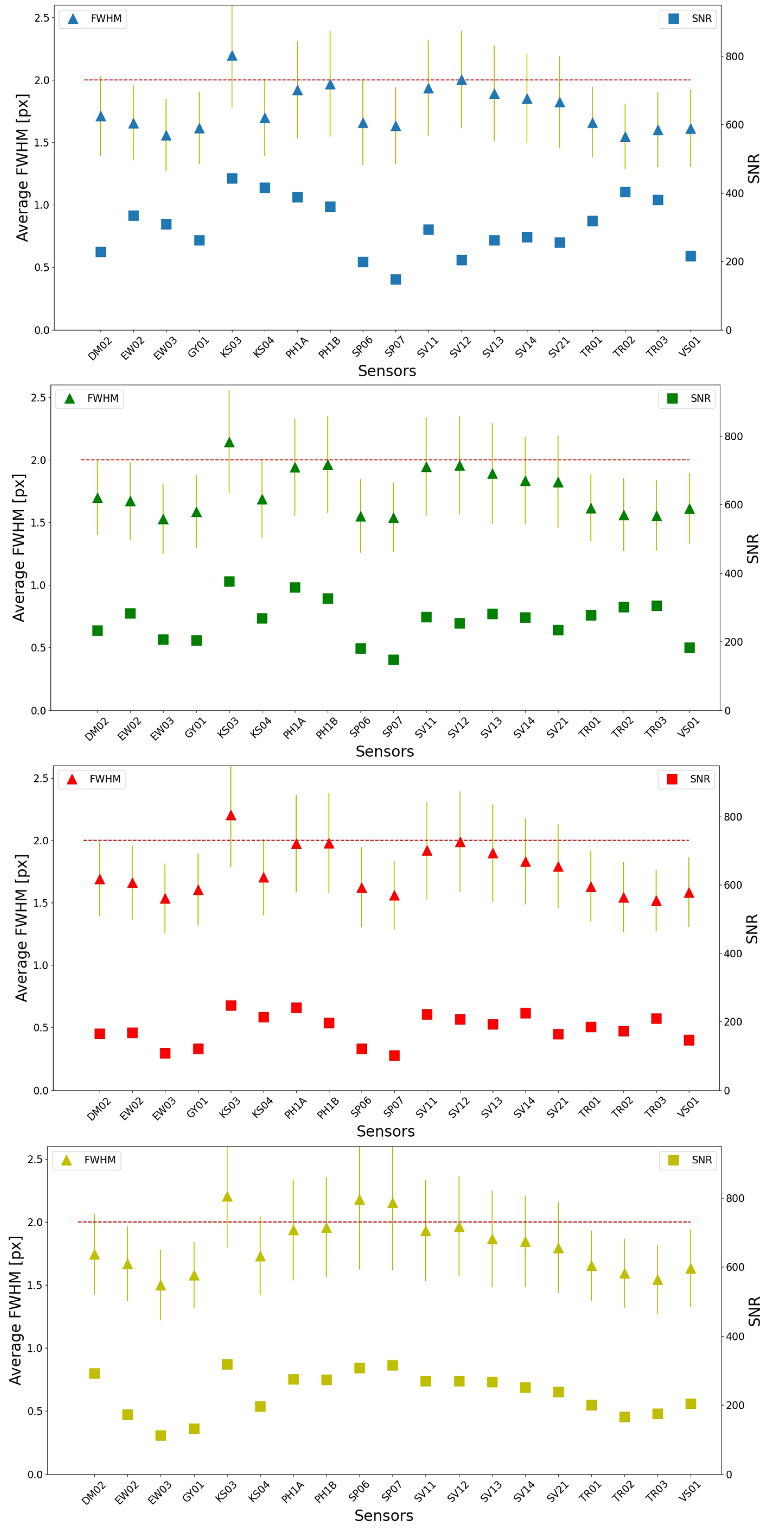
3.1. FWHM and SNR Estimation

The results of the simultaneous FWHM and SNR assessment carried out on the subsets of the VHR_IMAGE_2021 products are shown in the following tables, each of which is dedicated to a specific spectral channel:
  • Table 4 contains the results for the BLUE channels;
  • Table 5 contains the results for the GREEN channels;
  • Table 6 contains the results for the RED channels;
  • Table 7 contains the results for the NIR channels;
Each table contains the total edge count, which represents the total number of eligible edges processed by the AEM, the FWHM mean ( μ ) value, which represents the mean of all the FWHM values calculated for all eligible edges, the FWHM standard deviation ( σ ), calculated as the standard deviation of all the FWHM values of all the eligible edges, and the image SNR, estimated using Equation (5).
In order to enable an easy inter-band comparison for each product, Figure 3 shows the estimated values of both the FWHM (represented by the blue triangles) with their standard deviations (represented by the vertical amber lines) and the SNR (represented by the blue squares) for each band of each product; the horizontal dashed red line represents the 2.00 pixels FWHM threshold, which marks the boundary between balanced and blurry images according to [13].
Furthermore, the results were also investigated after aggregating the edges processed in all the selected images of a given mission, in order to characterise each product with a single quality indicator. The average of all the FWHM (represented by blue triangles) and SNR (represented by black squares) mean values evaluated for each band of each product grouped by product are shown in Figure 4, while the numeric values of the results are reported in Table 8. In addition, Table 8 also reports the product GSD/PS ratio, which was evaluated by averaging the information declared in the metadata file of each product.
Figure 5 preliminarily depicts the relationship between the evaluated FWHM and SNR mean values, by showing the SNR means directly against the corresponding FWHM means for each considered VHR_IMAGE_2021 product.

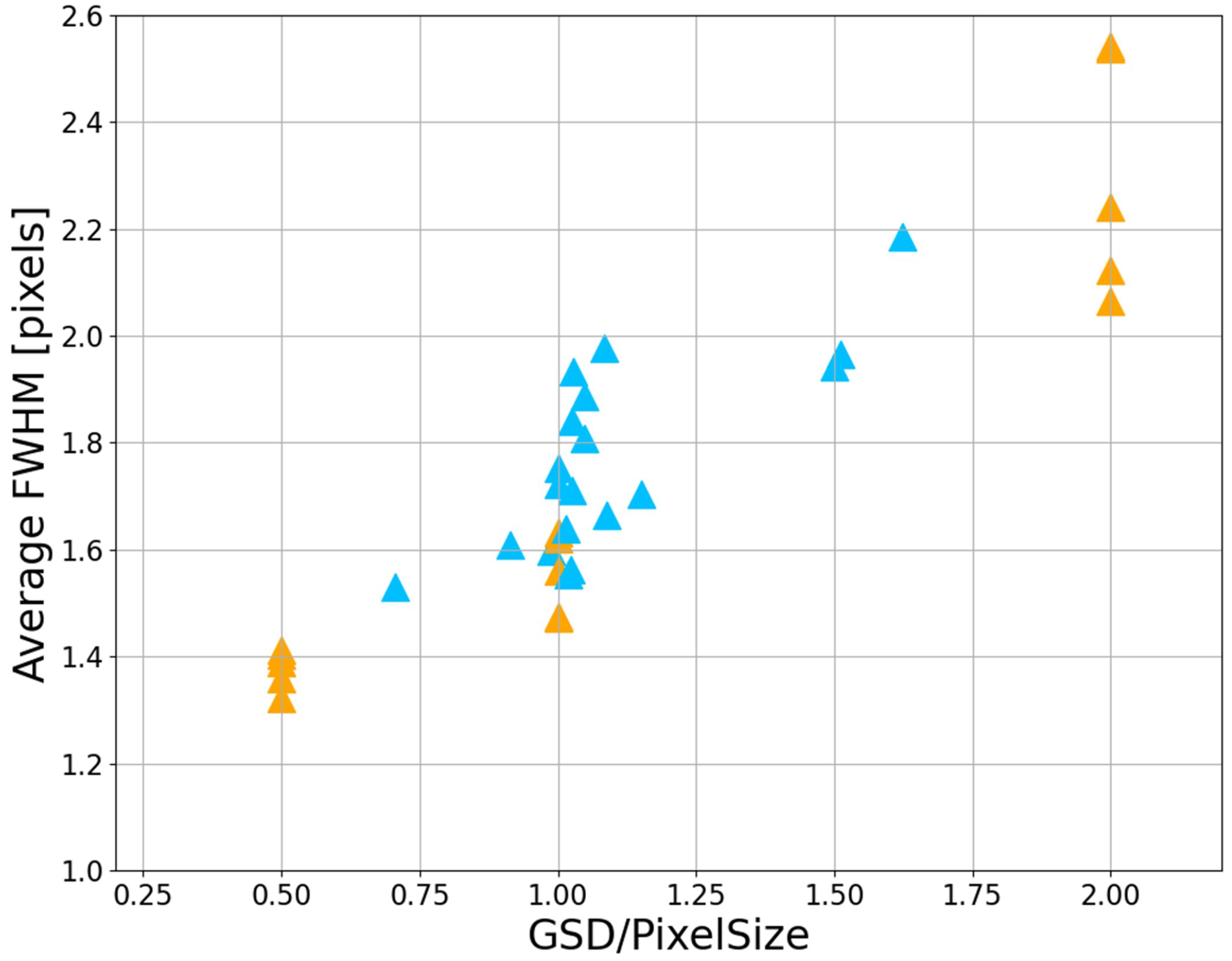
3.2. FWHM and SNR Assessment against GSD/PS Ratio

All the FWHM and SNR metrics evaluated in the previous section are hereby plotted against their respective GSD/PS ratios. Figure 6 shows the estimated product FWHM against the product GSD/PS ratios and Figure 7 shows the estimated product SNR against the respective product GSD/PS ratio.

4. Discussion

The results shown in Section 3 are hereby discussed following the same structure. As mentioned in [4], the scarcity of similar studies published in peer-reviewed international and scientific journals makes it difficult to find data to compare our results with. For this reason, our findings were verified through direct visual inspection of the products.

4.1. FWHM and SNR Generic Assessment

As shown in Figure 3, the AEM returned consistent results across the four analysed spectral bands for most of the products, with the SPOT-6/7 TrueSharp products being the only exceptions; in these two latter cases, the FWHM mean values obtained for the NIR band were noticeably higher than the corresponding RED, GREEN and BLUE bands, implying that the NIR band is significantly blurrier than the visible bands. Some amount of blurriness in SPOT TrueSharp products was noted in the scientific literature at the borders of homogeneous parcels [34]. The added blur in the NIR band is also evident through direct visual inspection of the product. Figure 8 shows a detail of a SP06 product (i.e., the SP06_04 product reported in Table A1) over an agricultural area, placing the RED and the NIR band side by side. We can therefore conclude that the AEM assessment of the SPOT TrueSharp channels correctly shows a worse sharpness performance of the NIR channel compared to its BLUE, GREEN and RED channels.
At the same time, the mean value of the SNR of the SPOT-6/7 NIR band is noticeably higher than the SNR of the BLUE, GREEN and RED bands, which would imply that the NIR band has a better radiometric performance. While counter-intuitive, an increase in SNR can be associated with a blurrier image, i.e., with a worse sharpness performance: this worse sharpness performance tends to cut off subtle variations in the signal, affecting the signal standard deviation much more than the signal intensity. Consequently, a blurrier image may return higher SNR than a sharper image acquired over the same area simply because the blur will reduce the standard deviation of the signal. In addition, the higher SNR could also be explained by the fact that the AEM was mainly applied over agricultural areas, and it is well known that, under normal conditions, the vegetation reflects more in the NIR band than in the visible bands [38]. This will translate to higher average signal values over vegetated areas, and, disregarding the effect that additional blur may have on the signal standard deviation, into a higher SNR. Apart from these considerations regarding the NIR band, we can state that the sharpness performance of SPOT6/7 TrueSharp products in the BLUE, GREEN and RED channels is comparable to that of other products considered in this analysis, while their SNR tends to be lower than the average of the other products.
While sharpness performance is rather consistent across the four analysed spectral bands, the BLUE band consistently performed better than the others in terms of SNR. As already noted in [4], the NIR and RED bands are naturally more contrasted with respect to the GREEN and BLUE bands in vegetated areas, which are the ones targeted by the AEM. This is mostly due to a combination of atmospheric effect and natural surface spectral reflectance characteristics [39]. Furthermore, the BLUE band is more affected by the Rayleigh scattering with respect to the GREEN, RED and NIR bands. Rayleigh scattering is the dominant scattering process in the upper atmosphere, with a stronger effect at shorter wavelengths [38]. For these reasons, subtle variations of the signal in the BLUE band might be more difficult to measure, leading to lower standard deviations and consequently higher estimated SNR values.
Nevertheless, the results summarised in Figure 4 and Table 8 show that the sharpness performance of most of the analysed products can be considered “balanced” according to the quality classification criteria [13], with a mean FWHM between 1.5 and 2.0 pixels. The FWHM standard deviations are rather stable at around 0.3 pixels. This trend in the results was also confirmed through the visual assessment of the products, during which no significant blurring was noted.
Comparing the performance of different products shows how SuperView-2 imagery (SV21) performs better than their SuperView-1 predecessors (i.e., SV11, SV12, SV13 and SV14), with performance improving consistently from each product generation to the next, going from slightly blurry to more and more balanced, while maintaining stable SNR values. These image quality improvements can easily be traced back to the technical advances brought on by the SuperView-2 mission with respect to the SuperView-1 satellite constellation, primarily in terms of GSD: the multi-spectral instrument of SuperView-2 has a GSD of 1.68 m at nadir [40], against the 2.00 m of its predecessor [41]. The perceived sharpness of the product definitely benefits from the improved GSD when the product is resampled to a common PS of 2 m, as performed within the VHR_IMAGE_2021 project. This topic will be further investigated in the next section.
Figure 5 shows that the estimated FWHM and SNR mean values are characterised by a consistent trend with a good degree of correlation between the products. In other words, products with higher SNR (better radiometric performance) also tend to show higher FWHM (worse sharpness performance). This result is very important: users would naturally believe that a product with a higher SNR is always desirable, but this may come at the price of a reduced sharpness performance. In other words, this result highlights the importance of conducting comprehensive image quality assessments, which are not limited to the GSD of the imaging system and its SNR.

4.2. Image Quality Assessment: FWHM, SNR and GSD/PS Ratio

Figure 6 and Figure 7 show the relationship between the FWHM and the GSD/PS ratio and between the SNR and the GSD/PS ratio, respectively. In both cases, we can easily identify a trend. In the FWHM case, almost all samples fall into the area of the graph that contains “balanced” performance imagery, with FWHM values between 1.0 and 2.0, and ideally around 1.5. Most of the samples tend to fall on the blurrier side of the “balanced” area, i.e., in the 1.5–2.0 FWHM interval. This is not surprising, since blur can be naturally introduced in imagery by a number of natural effects, such as [1]:
  • Platform motion, causing jitter and smear;
  • Imperfections in the manufacturing of the optical system;
  • Finite slit size;
  • Random noise;
  • Atmospheric effects.
All these phenomena are taken into account and mitigated during the design phase, but cannot be completely eliminated. Aliasing, on the other hand, can be introduced in post-processing, for instance by sharpening algorithms [13,18], but in general it is mainly a sampling issue: an undersampled signal will be recorded as having a lower frequency content than the original [3], i.e., it will appear “jagged”. Therefore, it can be accounted for and prevented more easily than blur.
It is intuitive how higher GSD/PS ratios, i.e., smaller image PS values with respect to the GSD, will translate into a higher amount of pixels compared to the original samples, which will inevitably introduce more blur and cause a worse sharpness performance. This also explains the increasing SNR values with increasing GSD/PS ratios: the added blur masks subtle variations in the signal, reducing its standard variation, thus increasing the SNR. As expected, this result suggests that a stronger PS stressing of a product (i.e., providing data with a PS increasingly smaller than the native GSD of the sensor) will result in blurrier imagery [20], even though at the apparent benefit of a SNR increase. This trend is also consistent with the Generalized Image-Quality Equation (GIQE) structure [42]. The GIQE was designed specifically to relate measurable image quality parameters (which originally included GSD, image sharpness measured through MTF and SNR) to the National Imagery Interpretability Rating Scale (NIIRS). In turn, the NIIRS is a qualitative rating system for various types of imagery, which is based on the possibility of performing different types of tasks with a given image [43]. Similarly to our findings, the GIQE suggests that, past a certain level, an increasing SNR will not have a noticeable impact for optical data interpretation purposes [31]; in other words, considering the GIQE, the GSD and RER are the dominant terms in determining the image quality, while the SNR plays a secondary role [42,44,45,46].
In conclusion, it can be stated that there exists a directly proportional relationship between the FWHM and the GSD/PS ratio, and between the SNR and the GSD/PS ratio, implying that the increase/decrease in one parameter reflects into the increase/decrease in the other. Consequently, product curators may adjust the PS of their products to obtain better sharpness performance (i.e., by increasing the PS) or to obtain better radiometric performance (i.e., by decreasing the PS), and ideally they will be able to do so to obtain satisfactory performance in both aspects.
While sharpness is a spectrum between aliasing and blur, and its optimal “balanced” performance is quantified by the 1.5 pixel FWHM value [13], as previously explained it is more difficult to define a minimum threshold for the SNR. Nevertheless, in general we can state that the closer the FWHM is to 1.5 pixels, the higher the SNR, and the smaller the GSD, thus the better the overall image quality.

4.3. Investigating the SuperView-1 Outliers

The SuperView-1 missions stand out as outliers in the FWHM vs. GSD/PS graph in Figure 6: their average FWHM values are in the 1.8–2.0 pixels range, while all the other missions characterised by a similar GSD/PS ratio (i.e., GeoEye-01, WorldView-02) fall within the 1.55–1.75 range. At the same time, the SNR vs. GSD/PS graph in Figure 7 shows no noticeable deviation from the norm for these platforms. To investigate this finding, we performed an additional sharpness assessment considering only overlapping areas covered by SuperView-01, GeoEye-01, WorldView-02 and Kompsat-03 products; the involved products are described in detail in the Appendix A in Table A2, while Table 9 summarises the results of the analysis: the “FWHM μ (subset)” column contains the average FWHM value calculated in the common area for the amount of edges reported in the “Total Edge Count” column. The “FWHM μ (product)” column reports the average FWHM which was previously obtained for the entire product and reported in Table 8, in order to easily verify if the results obtained for the common area significantly deviate from the results obtained at the product level.
In general, the sharpness performance evaluated over the common area returned results coherent with the global ones: the differences between the FWHM average calculated for the image subset and for all the images of the associated mission are much smaller than the standard deviation values shown in Table 8. In particular, the SuperView-1 products showed FWHM values greater than the ones obtained by the other considered products with a similar GSD/PS ratio. This performance difference can be attributed to the better native GSD of the GeoEye-1 [47] and WorldView-2 [48] sensors with respect to the SuperView-1 ones [41]. Since all products in the VHR_IMAGE_2021 are resampled to a common resolution of 2 m, products with a lower (better) native GSD are expected to show a better sharpness performance than products with a higher (worse) GSD.
It should be noted that the analysed products do not have similar GSD/PS ratios natively: GeoEye-1 has a GSD at nadir of 1.64 m, Kompsat-3 of 2.8 m and WorldView-2 of 1.8 m, while SuperView-1 has a GSD at nadir of 2.00 m. Since all analysed images were resampled to a PS of 2 m, the similar GSD/PS ratios considered in this additional experiment were due to similar effective GSD values. The effective GSD depends on the acquisition geometry of each image, which was not always nadir pointing or near-nadir pointing, increasing the effective GSD with respect to the nadir value. The effective GSD depends on several parameters that were not considered in the current analysis (e.g., the height of the satellite platform, the acquisition Off-Nadir Angle (ONA), etc.), which is dedicated to the image product level. In particular, the ONA of the analysed SuperView-1 products was generally smaller than the ONA of the analysed GeoEye-1 and WorldView-2 products, significantly contributing to obtaining similar effective GSD values compared to satellites with a smaller GSD at nadir. Therefore, under the specific conditions determined by the characteristics of the VHR_IMAGE_2021 dataset, which targets products at a PS of 2 or 4 m, it is not surprising to find that GeoEye-1 and WorldView-2 products show a significantly better sharpness performance than SuperView-1 products, since the former can benefit from a higher native GSD. The opposite consideration applies to the Kompsat-3 case, which suffers from the highest at-nadir GSD of all the platforms considered in this analysis. This case study serves as an example to show the utility of performing an assessment at the image level, since it allows us to judge the overall image quality under operational conditions, rather than in terms of technical characteristics which are not necessarily representative of actual use cases.
This performance difference was further investigated through visual inspection of the products, in order to verify if the image quality assessed by the AEM aligns with the visually apparent performance of the images; Figure 9, Figure 10 and Figure 11 portray the RGB crops of the common areas of each analysed product pair, i.e., SV11 and GY01, SV12 and KS03 and SV14 and EW02. In Figure 9, the better sharpness performance of the GeoEye product is immediately apparent from the contours of the roads and of the buildings, which appear better defined than those portrayed by SuperView-1. However, the better GeoEye-1 performance is more noticeable in how it makes it much easier to distinguish the outline of the trees against the grassy understory compared to the SuperView-1 image. In this case, the contrast between the tree canopy and the grass below it is much lower than the contrast between the rooftop of a building and its surroundings, making the performance difference between the two satellites more evident. In Figure 10, the performance difference between the SuperView-1 image and the Kompsat-3 image is more noticeable from the contours of the smaller objects scattered in the portrayed area, such as the trees at the side of the road in the bottom right. Finally, in Figure 11 the WorldView-2 image is noticeably sharper than its SuperView-1 counterpart, especially if we focus on the sides of the roads and on the roofs of the smaller buildings.
The visual inspection confirms the capability of the AEM to quantify the difference in performance between different image products, even when limiting the analysis to small subsets and therefore when relying on a reduced number of edges to perform the analysis.

4.4. Expanding the GSD/PS Range: A Synthetic Experiment with Landsat and Sentinel Products

To further verify the strictly proportional dependence between both the estimated FWHM and SNR mean values with respect to the GSD/PS ratio shown in Figure 6 and Figure 7, we performed a synthetic experiment: we considered Landsat-7/8/9 and Sentinel-2A/B products, which still have a GSD/PS ratio equal to 1.00, and up- and down-sampled them using a nearest neighbour algorithm in order to increase the range of GSD/PS ratio values from 0.50 to 2.00. Using the nearest neighbour algorithm, ideally, allows to intervene only on the sampling, preserving the original pixel values where possible. This, compared to other resampling algorithms, allows us to alter the sharpness performance of the original image as little as possible.
Specifically, the analysis included the following products:
  • Landsat-7/8/9 products: original PS of 30 m (i.e., GSD/PS = 1.00), up-sampled to 15 m (i.e., GSD/PS = 2.00) and down-sampled to 60 m (i.e., GSD/PS = 0.50);
  • Sentinel-2 products: original PS of 10 m (i.e., GSD/PS = 1.00), up-sampled to 5 m (i.e., GSD/PS = 2.00) and down-sampled to 20 m (i.e., GSD/PS = 0.5).
Figure 12 and Figure 13 show the average of all the FWHM and SNR mean values evaluated for the VHR_IMAGE_2021 dataset (blue triangles) and for the Landsat-7/8/9 and Sentinel-2A/B dataset (amber triangles) against their GSD/PS values. As performed in Figure 6 and Figure 7, the results were obtained after aggregating the edges detected in all the selected images for each product, i.e., the final metrics are calculated as the mean of the means of the quality metrics of each band of each product, and then grouped by product. The numeric values of the results are also summarised in Table 10.
The results obtained for the Landsat-8 products in terms of FWHM show an average of 1.48 pixels with a standard deviation of 0.22. These results align with those obtained with the previous semi-automatic version of this method [4], implying that the AEM remained consistent with its predecessor.
First of all, it is noticeable how the amount of retrieved edges is almost always highest at the native resolution of both Landsat and Sentinel images. While this may seem counter-intuitive at first, the explanation is pretty straightforward. Down-sampled images (i.e., 60 m resolution Landsat images and 20 m resolution Sentinel images) have a quarter of the original pixels to work with; this implies that the number of candidate edges within the imaged landscape is reduced accordingly. At the same time, if the target edge length of the algorithm is not altered compared to the native resolution images, even with the same amount of candidate edges, the larger PS will inevitably exclude all the physical edges which are not long enough. Conversely, the up-sampled images (i.e., 15 m resolution Landsat images and 5 m resolution Sentinel images) will suffer from the increased blur in the selection of candidate edges, which will have more difficulty in clearing all the steps of the edge selection. Unsurprisingly, the decrease in number of eligible edges affects the down-sampled images much more than the up-sampled ones. When necessary, the issue can be mitigated by adjusting the target edge length. The importance of being able to adjust this parameter was explicitly stated by [5]. In practice, the target edge length can be increased for images with a small PS, in order to limit the amount of edges processed in cases where this amount tends to be excessively high. Conversely, the target edge length can be decreased for images with a large PS, in order to relax the edge eligibility checks. Nevertheless, the automation of the AEM generally results in very high eligible edge counts, which made adjusting the target edge length unnecessary for this synthetic experiment. The stability of the results is shown by the standard deviation values shown alongside the FWHM means reported in Table 10, even when the edge count is in the hundreds, rather than in the thousands or tens of thousands.
At first sight, the SNR values estimated by the AEM show an unexpected result: Landsat-7 appears to be less noisy than Landsat-8 and Landsat-9. Upon further analysis, this result can probably be ascribed to Landsat-7’s lower native bit depth: Landsat-7 data have a bit depth of 8 bits, against the 12 and 14 bits of Landsat-8 and Landsat-9, respectively. Sometimes the bit depth is used as the sole parameter to describe the radiometric resolution of a system, but this is misleading, since having a higher number of quantisation bits does not necessarily imply that the sensor is able to detect smaller radiance changes, due to the presence of noise and due to the characteristics of the sensor itself [7]. In our case, i.e., at the image level, a lower bit depth will translate into products with an inferior capability to reproduce subtle variations in the signal, which will lead to smaller standard deviations and consequently higher SNR values at a given signal level.
The results of the expanded GSD/PS range analysis shown in Figure 12 and Figure 13 confirm the general trend already noticed in a more restricted range in Figure 6 and Figure 7. In particular, it can be stated that the greater (smaller) the GSD/PS ratio, the greater (smaller) the FWHM and SNR values. While this result was expected for the sharpness assessment, since at a given PS it is natural that a smaller GSD will lead to sharper imagery, it was more surprising for the SNR. As previously stated, this can be explained in terms of the effect that a higher GSD/PS ratio has on the variations of the signal over HAs, which determine the SNR through the standard deviation term. Let us fix the GSD at a certain value and progressively decrease the PS: this will lead to higher and higher GSD/PS ratios and to progressively blurrier images. While the measured and perceived sharpness performance will inevitably worsen, the added blur will also tend to mask subtle variations in the signal over HAs, which will result in lower standard deviations of the signal and consequently in higher measured SNR values at a given signal level. For this reason, even if the SNR is a fundamental quality parameter for optical image products, it should always be considered together with the FWHM parameter (or with an equivalent sharpness metric), in order to provide a more comprehensive assessment of the overall image quality.

5. Conclusions

The analysis carried out in this paper focused on the study of the mutual relationships between the overall quality of optical EO images with respect to the product resampling (in terms of GSD/PS ratio), image sharpness (in terms of FWHM) and image radiometric quality (in terms of SNR). For such a purpose, the study started with a joint sharpness and SNR assessment of a wide set of optical EO data. In particular, this study analysed a number of VHR optical satellite image products belonging to the VHR_IMAGE_2021 dataset [23], which are distributed with different GSD and PS values. The overall image quality of these products was assessed in terms of image sharpness (using the FWHM as a metric) and in terms of radiometric quality (using the SNR as a metric) by means of the AEM (described in detail in [20]), which allowed us to extract both metrics concurrently and coherently using the same methodology.
Concerning the sharpness assessment, the results were interpreted according to the USGS guidelines [13], and the performance of the vast majority of the analysed products was rated as “balanced”, since the associated average FWHM values ranged between 1.5 and 2.0 pixels. A few products were closer to the “blurry” class, with an average FWHM around or slightly above 2.0 pixels; the trend of the results was also confirmed through visual inspection of the data, which always confirmed the capability of the AEM to reliably measure even small differences in performance.
The analysis showed that the estimated FWHM and SNR parameters were characterised by a good degree of correlation: as expected, the FWHM and the SNR are representative of the quality of an optical EO image in a complementary way. Images with higher FWHM (i.e., worse sharpness performance) also tend to have higher SNR (i.e., better radiometric performance). Therefore, the SNR alone is not sufficient to describe the overall quality of a given product, but should always be accompanied by a corresponding sharpness metric such as the FWHM.
Furthermore, the results highlighted the relationship between the estimated FWHM and SNR metrics with respect to the product resampling (GSD/PS ratio). In particular, the analysis of the results showed how the increase (decrease) of one parameter reflected into the increase (decrease) of the other; indeed, the products with a high value of FWHM and SNR were characterised by a high value of GSD/PS ratio. As expected, this suggests that submitting imagery to an excessive PS stressing process (i.e., distributing imagery with a PS smaller than the native GSD of the sensor) will result in a worsening of the sharpness performance, even if at the apparent benefit of an increased SNR. Consequently, optical EO product users should always take into account this aspect when selecting which products to use, according to their specific needs and to the specific application.
In other words, the results showed the difficulty in quantifying the quality of optical EO data using a single parameter, and highlighted how the concept of image quality depends on multiple factors, suitable to describe different aspects of the problem and on their mutual relationships. Within this context, it can be stated that a comprehensive assessment of GSD/PS ratio, FWHM (or of an equivalent sharpness metric) and SNR provides a complete description of the overall image quality of a given optical image product, i.e., of the capability to distinguish ground targets in a single image channel of a specific optical image product. At a given GSD/PS ratio, the more “balanced” the sharpness (i.e., the closer the FWHM to 1.5), the higher the SNR, and thus the better the overall image quality.
This work represents a first attempt to investigate the mutual relationship between the overall quality of optical EO images with respect to the product GSD/PS ratio, image sharpness and SNR. The analysis highlighted the complexity of the topic and the importance and added value of relying on automatic and self-consistent methodology. In the future, further analyses will be dedicated to investigating the effect that super-resolution algorithms have on the quality of the resulting product, and also to analyse the performance of Virtual Constellations (VC) such as the Landsat-Sentinel VC proposed by [49]. The AEM may also be exploited to monitor the performance of satellite constellations, in particular those composed of small satellites, in order to determine whether the performance of the different satellites is coherent and whether or not it degrades with the passage of time.

Author Contributions

Conceptualization, V.P., L.C., F.F., G.L. and C.S.; Methodology, V.P., L.C., F.F., G.L. and C.S.; Software, V.P., L.C. and F.F.; Validation, V.P., L.C. and F.F.; writing—original draft preparation, V.P. and F.F.; writing—review and editing, V.P., L.C., F.F., G.L., C.S. and V.B. All authors have read and agreed to the published version of the manuscript.

Funding

The activities were carried out by the Copernicus Coordinated data Quality Control (CQC) service run by Serco Italia SpA and La Sapienza University of Rome within the European Space Agency (ESA) “PRISM” contract in the framework of the European Union’s Earth observation program “Copernicus”.

Data Availability Statement

The Landsat 7/8/9 data used for the analysis can be downloaded from https://earthexplorer.usgs.gov/ (accessed on 14 March 2024). The Sentinel-2A/B data used for the analysis can be downloaded from https://scihub.copernicus.eu/dhus/ (accessed on 14 March 2024). The VHR_IMAGE_2021 data used for the analysis can be downloaded from https://panda.copernicus.eu/web/cds-catalogue/panda (accessed on 14 March 2024).

Conflicts of Interest

The authors declare no conflict of interest.

Abbreviations

The following abbreviations are used in this manuscript:
AEMAutomatic Edge Method
CCMCopernicus Contributing Missions
CQCCoordinated Quality Control
DNDigital Number
EEAEuropean Economic Area
EMEdge Method
EOEarth Observation
ESFEdge Spread Function
FWHMFull-Width at Half-Maximum
GIQEGeneralized Image-Quality Equation
GSDGround Sampling Distance
HAHomogeneous Area
IFOVInstantaneous Field Of View
LSFLine Spread Function
MTFModulation Transfer Function
NIIRSNational Imagery Interpretability Rating Scale
NIRNear-Infrared
ONAOff-Nadir Angle
PSPixel Size
PSFPoint Spread Function
RERRelative Edge Response
RGBRed, Green and Blue
SNRSignal-to-Noise Ratio
USGSUnited States Geological Survey
VCVirtual Constellation
VHRVery High Resolution

Appendix A

Table A1 lists all the products considered in this work reporting the file name, GSD and PS for each product.
Table A1. List of the products involved in the sharpness and SNR analysis.
MissionProduct IDProduct NameGSD [m]PS [m]
DEIMOS-2DM02_01DM02_HRS_MS4_1C_20210616T101753_20210616T101755_TOU_1234_6ad44.194.00
DM02_02DM02_HRS_MS4_1C_20210617T085910_20210617T085912_TOU_1234_9a364.004.00
DM02_03DM02_HRS_MS4_1C_20210717T083735_20210717T083737_TOU_1234_7e804.064.00
DM02_04DM02_HRS_MS4_1C_20210730T084952_20210730T084955_TOU_1234_b6294.014.00
DM02_05DM02_HRS_MS4_1C_20210731T072451_20210731T072454_TOU_1234_1aa94.234.00
WORLDVIEWEW02_01EW02_WV1_MS4_OR_20200609T084534_20200609T084540_TOU_1234_873f2.432.00
EW02_02EW02_WV1_MS4_OR_20210610T103006_20210610T103017_TOU_1234_59402.062.00
EW02_03EW02_WV1_MS4_OR_20210704T104516_20210704T104524_TOU_1234_46fd2.312.00
EW02_04EW02_WV1_MS4_OR_20210807T095542_20210807T095545_TOU_1234_c0bf1.902.00
EW03_01EW03_WV3_MS4_OR_20200818T102631_20200818T102654_TOU_1234_5c881.242.00
EW03_02EW03_WV3_MS4_OR_20210719T101306_20210719T101336_TOU_1234_79d91.362.00
EW03_03EW03_WV3_MS4_OR_20210721T090836_20210721T090847_TOU_1234_140e1.342.00
EW03_04EW03_WV3_MS4_OR_20210925T112632_20210925T112644_TOU_1234_2f521.712.00
GEOEYEGY01_01GY01_GIS_MS4_OR_20200606T100416_20200606T100423_TOU_1234_dc9d2.182.00
GY01_02GY01_GIS_MS4_OR_20200629T104347_20200629T104355_TOU_1234_469f1.912.00
GY01_03GY01_GIS_MS4_OR_20200908T090225_20200908T090228_TOU_1234_c95f1.952.00
GY01_04GY01_GIS_MS4_OR_20210703T102536_20210703T102553_TOU_1234_73261.952.00
GY01_05GY01_GIS_MS4_OR_20210903T095209_20210903T095215_TOU_1234_f6941.882.00
KOMPSATKS03_01KS03_AIS_MSP_1G_20200609T114244_20200609T114246_TOU_1234_82ef3.002.00
KS03_02KS03_AIS_MSP_1G_20200625T120729_20200625T120731_TOU_1234_46e42.872.00
KS03_03KS03_AIS_MSP_1G_20200801T125053_20200801T125055_TOU_1234_20693.772.00
KS03_04KS03_AIS_MSP_1G_20200914T130815_20200914T130817_TOU_1234_2cc33.762.00
KS03_05KS03_AIS_MSP_1G_20210715T111238_20210715T111240_TOU_1234_cb092.832.00
KS04_01KS04_AIS_MSP_1G_20200813T121309_20200813T121311_TOU_1234_32812.212.00
KS04_02KS04_AIS_MSP_1G_20200912T130938_20200912T130939_TOU_1234_d2502.312.00
KS04_03KS04_AIS_MSP_1G_20210624T112153_20210624T112155_TOU_1234_e7a22.222.00
KS04_04KS04_AIS_MSP_1G_20210624T112409_20210624T112410_TOU_1234_fc8b2.472.00
PLEIADESPH1A_01PH1A_PHR_MS___3_20200523T090432_20200523T090432_TOU_1234_82cf2.812.00
PH1A_02PH1A_PHR_MS___3_20200813T083340_20200813T083346_TOU_1234_52ca3.062.00
PH1A_03PH1A_PHR_MS___3_20200901T101529_20200901T101535_TOU_1234_3ebf3.032.00
PH1A_04PH1A_PHR_MS___3_20200914T110429_20200914T110429_TOU_1234_60172.872.00
PH1A_05PH1A_PHR_MS___3_20210906T110647_20210906T110652_TOU_1234_80473.222.00
PH1B_01PH1B_PHR_MS___3_20210709T102247_20210709T102251_TOU_1234_57d42.802.00
PH1B_02PH1B_PHR_MS___3_20210718T082612_20210718T082618_TOU_1234_91352.812.00
PH1B_03PH1B_PHR_MS___3_20210727T112528_20210727T112534_TOU_1234_0c302.822.00
PH1B_04PH1B_PHR_MS___3_20210818T101425_20210818T101433_TOU_1234_20e33.192.00
PH1B_05PH1B_PHR_MS___3_20210921T105222_20210921T105230_TOU_1234_bf1e3.502.00
SPOTSP06_01SP06_NAO_MS4__3_20210616T102257_20210616T102307_TOU_1234_fe334.004.00
SP06_02SP06_NAO_MS4__3_20210624T110229_20210624T110301_TOU_1234_d2724.004.00
SP06_03SP06_NAO_MS4__3_20210714T083035_20210714T083045_TOU_1234_1c5e4.004.00
SP06_04SP06_NAO_MS4__3_20210814T101933_20210814T101942_TOU_1234_918d4.004.00
SP07_01SP07_NAO_MS4__3_20200630T102323_20200630T102323_TOU_1234_fbdc4.004.00
SP07_02SP07_NAO_MS4__3_20210610T101730_20210610T101738_TOU_1234_071c4.004.00
SP07_03SP07_NAO_MS4__3_20210611T110012_20210611T110045_TOU_1234_86cf4.004.00
SP07_04SP07_NAO_MS4__3_20210727T082941_20210727T082959_TOU_1234_1fc84.004.00
SUPERVIEW-1SV11_01SW00_OPT_MS4_1C_20200725T112833_20200725T112835_TOU_1234_13332.002.00
SV11_02SW00_OPT_MS4_1C_20210622T081606_20210622T081608_TOU_1234_3ebc2.062.00
SV11_03SW00_OPT_MS4_1C_20210907T092821_20210907T092823_TOU_1234_8d842.072.00
SV11_04SW00_OPT_MS4_1C_20210923T103134_20210923T103136_TOU_1234_99d52.092.00
SV12_01SW00_OPT_MS4_1C_20200721T112528_20200721T112530_TOU_1234_5bb02.082.00
SV12_02SW00_OPT_MS4_1C_20200810T114626_20200810T114628_TOU_1234_135d2.192.00
SV12_03SW00_OPT_MS4_1C_20210705T090341_20210705T090343_TOU_1234_a9632.012.00
SV12_04SW00_OPT_MS4_1C_20211003T115354_20211003T115356_TOU_1234_acd72.392.00
SV13_01SW00_OPT_MS4_1C_20200709T095313_20200709T095315_TOU_1234_5b572.002.00
SV13_02SW00_OPT_MS4_1C_20210602T104919_20210602T104922_TOU_1234_7d742.242.00
SV13_03SW00_OPT_MS4_1C_20210624T103220_20210624T103222_TOU_1234_88de2.012.00
SV13_04SW00_OPT_MS4_1C_20210909T100805_20210909T100807_TOU_1234_525f2.132.00
SV14_01SW00_OPT_MS4_1C_20200710T102057_20200710T102059_TOU_1234_d7202.052.00
SV14_02SW00_OPT_MS4_1C_20210629T114234_20210629T114236_TOU_1234_85302.062.00
SV14_03SW00_OPT_MS4_1C_20210706T100258_20210706T100301_TOU_1234_3cf52.092.00
SV14_04SW00_OPT_MS4_1C_20210803T082311_20210803T082313_TOU_1234_b5eb2.012.00
SUPERVIEW-2SV21_01SW00_OPT_MS4_1C_20210707T100020_20210707T100023_TOU_1234_be4a2.042.00
SV21_02SW00_OPT_MS4_1C_20210731T094046_20210731T094049_TOU_1234_1f362.072.00
SV21_03SW00_OPT_MS4_1C_20210804T080013_20210804T080016_TOU_1234_98e42.132.00
SV21_04SW00_OPT_MS4_1C_20210907T113148_20210907T113151_TOU_1234_08332.122.00
SV21_05SW00_OPT_MS4_1C_20210910T093006_20210910T093009_TOU_1234_8a032.132.00
TRIPLESATTR01_01TR00_VHI_MS4_1C_20200704T071337_20200704T071340_TOU_1234_731f4.154.00
TR01_02TR00_VHI_MS4_1C_20210606T081823_20210606T081826_TOU_1234_4fde4.044.00
TR01_03TR00_VHI_MS4_1C_20210606T081826_20210606T081830_TOU_1234_99114.034.00
TR01_04TR00_VHI_MS4_1C_20210920T094216_20210920T094220_TOU_1234_03924.024.00
TR02_01TR00_VHI_MS4_1C_20210605T082416_20210605T082420_TOU_1234_3e9c4.004.00
TR02_02TR00_VHI_MS4_1C_20210630T080542_20210630T080546_TOU_1234_b8e84.084.00
TR02_03TR00_VHI_MS4_1C_20210630T080552_20210630T080556_TOU_1234_28c74.094.00
TR02_04TR00_VHI_MS4_1C_20210711T080456_20210711T080459_TOU_1234_a1c24.224.00
TRIPLESATTR03_01TR00_VHI_MS4_1C_20210622T082010_20210622T082014_TOU_1234_8f504.054.00
TR03_02TR00_VHI_MS4_1C_20210629T081102_20210629T081105_TOU_1234_5dd14.014.00
TR03_03TR00_VHI_MS4_1C_20210713T075220_20210713T075224_TOU_1234_a50b4.194.00
TR03_04TR00_VHI_MS4_1C_20210808T075943_20210808T075947_TOU_1234_a8084.074.00
VISION-1VS01_01VS01_S14_MS4__3_20200901T095846_20200901T095858_TOU_1234_17083.734.00
VS01_02VS01_S14_MS4__3_20210603T091123_20210603T091144_TOU_1234_6caa3.834.00
VS01_03VS01_S14_MS4__3_20210709T075029_20210709T075050_TOU_1234_71e23.564.00
VS01_04VS01_S14_MS4__3_20210801T082843_20210801T082934_TOU_1234_95fa3.594.00
VS01_05VS01_S14_MS4__3_20210805T071433_20210805T071448_TOU_1234_bb173.554.00
LANDSAT-7LE07_01LE07_L1TP_192029_20000706_20200918_02_T13030
LE07_02LE07_L1TP_199026_20000824_20200917_02_T13030
LE07_03LE07_L1TP_200033_20000831_20211120_02_T13030
LE07_04LE07_L1TP_201023_20000619_20200918_02_T13030
LANDSAT-8LC08_01LC08_L1TP_192029_20140806_20200911_02_T13030
LC08_02LC08_L1TP_199026_20140519_20200911_02_T13030
LC08_03LC08_L1TP_200033_20140713_20200911_02_T13030
LC08_04LC08_L1TP_201023_20140517_20200911_02_T13030
LANDSAT-9LC09_01LC09_L1TP_192029_20220703_20230408_02_T13030
LC09_02LC09_L1TP_199026_20220517_20230416_02_T13030
LC09_03LC09_L1TP_200033_20220828_20230331_02_T13030
LC09_04LC09_L1TP_201023_20220718_20230407_02_T13030
SENTINEL-2AS2A_01S2A_MSIL1C_20160504T105622_N0202_R094_T31UDP_20160504T1059171010
S2A_02S2A_MSIL1C_20160606T110622_N0202_R137_T30UYD_20160606T1106241010
S2A_03S2A_MSIL1C_20160613T105622_N0202_R094_T30SVJ_20160613T1105591010
S2A_04S2A_MSIL1C_20160718T101032_N0204_R022_T32TQQ_20160718T1010281010
SENTINEL-2BS2B_01S2B_MSIL1C_20180506T105029_N0206_R051_T31UDP_20180509T1557091010
S2B_02S2B_MSIL1C_20180519T105619_N0206_R094_T30UYD_20180519T1320031010
S2B_03S2B_MSIL1C_20180708T105619_N0206_R094_T30SVJ_20180708T1344241010
S2B_04S2B_MSIL1C_20180822T101019_N0206_R022_T32TQQ_20180822T1424121010
Table A2 lists the Superview-1, GeoEye-1, Kompsat-3 and WorldView-2 products used for the sharpness and SNR assessment considering only a common area between the product pairs.
Table A2. List of the product pairs processed in the sharpness analysis over common area.
Product IDProduct Name
SV11_T01SW00_OPT_MS4_1C_20210923T103134_20210923T103136_TOU_1234_99d5
GY11_T01GY01_GIS_MS4_OR_20220617T105537_20220617T105555_TOU_1234_4955
SV12_T02SW00_OPT_MS4_1C_20200721T112528_20200721T112530_TOU_1234_5bb0
KS03_T02KS03_AIS_MSP_1G_20200623T123121_20200623T123123_TOU_1234_ba37
SV14_T03SW00_OPT_MS4_1C_20200710T102057_20200710T102059_TOU_1234_d720
EW02_T03EW02_WV1_MS4_OR_20210526T094717_20210526T094729_TOU_1234_7650

References

  1. Fiete, R.D. Image chain analysis for space imaging systems. J. Imaging Sci. Technol. 2007, 51, 103–109. [Google Scholar] [CrossRef]
  2. Joseph, G. How to Specify an Electro-optical Earth Observation Camera? A Review of the Terminologies Used and its Interpretation. J. Indian Soc. Remote Sens. 2020, 48, 171–180. [Google Scholar] [CrossRef]
  3. Holst, G.C. Electro-Optical Imaging System Performance; SPIE-International Society for Optical Engineering: Bellingham, WA, USA, 2008. [Google Scholar]
  4. Cenci, L.; Pampanoni, V.; Laneve, G.; Santella, C.; Boccia, V. Presenting a Semi-Automatic, Statistically-Based Approach to Assess the Sharpness Level of Optical Images from Natural Targets via the Edge Method. Case Study: The Landsat 8 OLI–L1T Data. Remote Sens. 2021, 13, 1593. [Google Scholar] [CrossRef]
  5. Crespi, M.; De Vendictis, L. A procedure for high resolution satellite imagery quality assessment. Sensors 2009, 9, 3289–3313. [Google Scholar] [CrossRef] [PubMed]
  6. Elachi, C.; Van Zyl, J.J. Introduction to the Physics and Techniques of Remote Sensing; John Wiley & Sons: Hoboken, NJ, USA, 2021. [Google Scholar]
  7. Joseph, G. Building Earth Observation Cameras; CRC Press: Boca Raton, FL, USA, 2015. [Google Scholar]
  8. Townshend, J.R. The spatial resolving power of earth resources satellites. Prog. Phys. Geogr. 1981, 5, 32–55. [Google Scholar] [CrossRef]
  9. Valenzuela, A.Q.; Reyes, J.C.G. Basic spatial resolution metrics for satellite imagers. IEEE Sens. J. 2019, 19, 4914–4922. [Google Scholar] [CrossRef]
  10. Lee, D.; Helder, D.; Christopherson, J.; Stensaas, G. Spatial Quality for Satellite Image Data and Landsat8 OLI Lunar Data. In Proceedings of the 38th CEOS Working Group Calibration Validation Plenary, College Park, MD, USA, 30 September–2 October 2014; Volume 30. [Google Scholar]
  11. Bakken, S.; Henriksen, M.B.; Birkeland, R.; Langer, D.D.; Oudijk, A.E.; Berg, S.; Pursley, Y.; Garrett, J.L.; Gran-Jansen, F.; Honoré-Livermore, E.; et al. Hypso-1 cubesat: First images and in-orbit characterization. Remote Sens. 2023, 15, 755. [Google Scholar] [CrossRef]
  12. Gallés, P.; Takáts, K.; Hernández-Cabronero, M.; Berga, D.; Pega, L.; Riordan-Chen, L.; Garcia, C.; Becker, G.; Garriga, A.; Bukva, A.; et al. A New Framework for Evaluating Image Quality Including Deep Learning Task Performances as a Proxy. IEEE J. Sel. Top. Appl. Earth Obs. Remote Sens. 2023, 17, 3285–3296. [Google Scholar] [CrossRef]
  13. Innovative Imaging and Research (I2R), Spatial Resolution Digital Imagery Guideline. 2023. Available online: https://www.i2rcorp.com/main-business-lines/sensor-hardware-design-support-services/spatial-resolution-digital-imagery-guideline (accessed on 14 March 2024).
  14. Schowengerdt, R.A. Remote Sensing: Models and Methods for Image Processing; Elsevier: Amsterdam, The Netherlands, 2006. [Google Scholar]
  15. Pampanoni, V.; Cenci, L.; Laneve, G.; Santella, C.; Boccia, V. On-orbit image sharpness assessment using the edge method: Methodological improvements for automatic edge identification and selection from natural targets. In Proceedings of the IGARSS 2020 IEEE International Geoscience and Remote Sensing Symposium, Waikoloa, HI, USA, 26 September–2 October 2020; IEEE: Piscataway, NJ, USA, 2020; pp. 6010–6013. [Google Scholar]
  16. Pampanoni, V.; Cenci, L.; Laneve, G.; Santella, C.; Boccia, V. A Fully Automatic Method for on-Orbit Sharpness Assessment: A Case Study Using Prisma Hyperspectral Satellite Images. In Proceedings of the IGARSS 2022 IEEE International Geoscience and Remote Sensing Symposium, Kuala Lumpur, Malaysia, 17–22 July 2022; IEEE: Piscataway, NJ, USA, 2022; pp. 7226–7229. [Google Scholar]
  17. Pagnutti, M.; Blonski, S.; Cramer, M.; Helder, D.; Holekamp, K.; Honkavaara, E.; Ryan, R. Targets, methods, and sites for assessing the in-flight spatial resolution of electro-optical data products. Can. J. Remote Sens. 2010, 36, 583–601. [Google Scholar] [CrossRef]
  18. Boreman, G.D. Modulation Transfer Function in Optical and Electro-Optical Systems; SPIE Press: Bellingham, WA, USA, 2001; Volume 4. [Google Scholar]
  19. Viallefont-Robinet, F.; Helder, D.; Fraisse, R.; Newbury, A.; van den Bergh, F.; Lee, D.; Saunier, S. Comparison of MTF measurements using edge method: Towards reference data set. Opt. Express 2018, 26, 33625–33648. [Google Scholar] [CrossRef]
  20. Fascetti, F.; Santella, C. Copernicus Coordinated Data Quality Control: Definition of an Automatic Methodology to Evaluate Signal-To-Noise Ratio on Optical Data. 2023. Available online: https://spacedata.copernicus.eu/documents/20123/212613/D-077_BGD_CQC_T7_PR19_AutomaticSNRMethodology_v1.0.pdf (accessed on 14 March 2024).
  21. Vescovi, F.D.; Haskell, L. Copernicus Data Quality Control—Technical Note Harmonisation of Optical Product Types—Geometric Corrections. 2016. Available online: https://spacedata.copernicus.eu/documents/20123/121286/CQC_TechnicalNote+(1).pdf (accessed on 14 March 2024).
  22. Cenci, L.; Galli, M.; Palumbo, G.; Sapia, L.; Santella, C.; Albinet, C. Describing the quality assessment workflow designed for DEM products distributed via the Copernicus Programme. Case study: The absolute vertical accuracy of the Copernicus DEM dataset in Spain. In Proceedings of the 2021 IEEE International Geoscience and Remote Sensing Symposium IGARSS, Brussels, Belgium, 11–16 July 2021; IEEE: Piscataway, NJ, USA, 2021; pp. 6143–6146. [Google Scholar]
  23. Optical VHR Coverage over Europe. 2022. Available online: https://spacedata.copernicus.eu/optical-vhr-coverage-over-europe-vhr_image_2021- (accessed on 14 March 2024).
  24. Choi, T.; Helder, D.L. Generic sensor modeling for modulation transfer function (MTF) estimation. In Proceedings of the Pecora 16, Global Priorities in Land Remote Sensing, Falls, South Dakota, 23–27 October 2005; Volume 16, pp. 23–27. [Google Scholar]
  25. Kabir, S.; Leigh, L.; Helder, D. Vicarious methodologies to assess and improve the quality of the optical remote sensing images: A critical review. Remote Sens. 2020, 12, 4029. [Google Scholar] [CrossRef]
  26. Duggin, M.; Sakhavat, H.; Lindsay, J. Systematic and random variations in thematic mapper digital radiance data. Photogramm. Eng. Remote Sens. 1985, 51, 1427–1434. [Google Scholar]
  27. Ren, H.; Du, C.; Liu, R.; Qin, Q.; Yan, G.; Li, Z.L.; Meng, J. Noise evaluation of early images for Landsat 8 Operational Land Imager. Opt. Express 2014, 22, 27270–27280. [Google Scholar] [CrossRef] [PubMed]
  28. Helder, D.; Choi, T.; Rangaswamy, M. In-flight characterization of spatial quality using point spread functions. Post-Launch Calibration Satell. Sens. 2004, 2, 151–170. [Google Scholar]
  29. Valenzuela, A.; Reyes, J. Comparative study of the different versions of the general image quality equation. ISPRS Ann. Photogramm. Remote Sens. Spat. Inf. Sci. 2019, 4, 493–500. [Google Scholar] [CrossRef]
  30. Qi, L.; Lee, Z.; Hu, C.; Wang, M. Requirement of minimal signal-to-noise ratios of ocean color sensors and uncertainties of ocean color products. J. Geophys. Res. Ocean. 2017, 122, 2595–2611. [Google Scholar] [CrossRef]
  31. Schott, J.R.; Gerace, A.; Woodcock, C.E.; Wang, S.; Zhu, Z.; Wynne, R.H.; Blinn, C.E. The impact of improved signal-to-noise ratios on algorithm performance: Case studies for Landsat class instruments. Remote Sens. Environ. 2016, 185, 37–45. [Google Scholar] [CrossRef]
  32. Cenci, L.; Galli, M.; Santella, C.; Boccia, V.; Albinet, C. Analyzing the Impact of the Different Instances of the Copernicus DEM Dataset on the Orthorectification of VHR Optical Data. In Proceedings of the IGARSS 2022–2022 IEEE International Geoscience and Remote Sensing Symposium, Kuala Lumpur, Malaysia, 17–22 July 2022; IEEE: Piscataway, NJ, USA, 2022; pp. 6001–6004. [Google Scholar]
  33. SPOT 6 and SPOT 7. Available online: https://spacedata.copernicus.eu/web/guest/spot-6-and-spot-7 (accessed on 14 March 2024).
  34. Aastrand, P.; Lemajic, S.; Wirnhardt, C. SPOT TrueSharp 4m; Comparison with Sentinel-2, PlanetScope, SPOT, and Pleiades—A Preliminary QUALITY Assessment; Publications Office of the European Union: Luxembourg, 2021. [Google Scholar] [CrossRef]
  35. Jacquemoud, S. Inversion of the PROSPECT+SAIL canopy reflectance model from AVIRIS equivalent spectra: Theoretical study. Remote Sens. Environ. 1993, 44, 281–292. [Google Scholar] [CrossRef]
  36. Landsat Science. Available online: https://landsat.gsfc.nasa.gov/ (accessed on 14 March 2024).
  37. Sentinel-2 Mission Guide. Available online: https://sentinels.copernicus.eu/web/sentinel/missions/sentinel-2 (accessed on 14 March 2024).
  38. Chuvieco, E. Fundamentals of Satellite Remote Sensing: An Environmental Approach; CRC Press: Boca Raton, FL, USA, 2020. [Google Scholar]
  39. Rees, G. Physical Principles of Remote Sensing; Cambridge University Press: Cambridge, UK, 2013. [Google Scholar]
  40. Superview-2 Satellite. Available online: http://en.spacewillinfo.com/uploads/soft/220425/1-220425132913.pdf (accessed on 14 March 2024).
  41. Superview-1 Satellite Imagery Product Guide. Available online: http://en.spacewillinfo.com/uploads/soft/210106/8-210106153503.pdf (accessed on 14 March 2024).
  42. Leachtenauer, J.C.; Malila, W.; Irvine, J.; Colburn, L.; Salvaggio, N. General image-quality equation: GIQE. Appl. Opt. 1997, 36, 8322–8328. [Google Scholar] [CrossRef]
  43. Irvine, J.M. National imagery interpretability rating scales (NIIRS): Overview and methodology. Airborne Reconnaiss. XXI 1997, 3128, 93–103. [Google Scholar]
  44. Li, L.; Luo, H.; Zhu, H. Estimation of the image interpretability of ZY-3 sensor corrected panchromatic nadir data. Remote Sens. 2014, 6, 4409–4429. [Google Scholar] [CrossRef]
  45. Thurman, S.T.; Fienup, J.R. Analysis of the general image quality equation. In Proceedings of the Visual Information Processing XVII, SPIE, Orlando, FL, USA, 18–19 March 2008; Volume 6978, pp. 102–114. [Google Scholar]
  46. Khetkeeree, S.; Liangrocapart, S. Satellite image restoration using adaptive high boost filter based on in-flight point spread function. Asian J. Geoinformat. 2018, 18, 15–17. [Google Scholar]
  47. GeoEye-1 Instruments. Available online: https://earth.esa.int/eogateway/missions/geoeye-1#instruments-section (accessed on 14 March 2024).
  48. WorldView-2 Instruments. Available online: https://earth.esa.int/eogateway/missions/worldview-2#instruments-section (accessed on 14 March 2024).
  49. Saunier, S.; Pflug, B.; Lobos, I.M.; Franch, B.; Louis, J.; De Los Reyes, R.; Debaecker, V.; Cadau, E.G.; Boccia, V.; Gascon, F.; et al. Sen2Like: Paving the way towards harmonization and fusion of optical data. Remote Sens. 2022, 14, 3855. [Google Scholar] [CrossRef]
Figure 1. Fitted Edge Spread Function and edge Signal-to-Noise Ratio. The estimation of the edge SNR is performed using the definition provided by [19,24]. The black horizontal lines show the width of the portions of the sides of the Edge Spread Function used for the purpose, which are calculated automatically using the positions which correspond to the 10% values of the Line Spread Function in its ascending and descending halves [20].
Remotesensing 16 01041 g001
Figure 2. Spatial distribution of the considered VHR_IMAGE_2021 products.
Remotesensing 16 01041 g002
Figure 3. FWHM (triangles) and SNR (squares) values averaged for each band of the products reported in Table 1. The standard deviation of each FWHM value is represented by the error bar centred on each triangle. The horizontal dashed red line represents the boundary between balanced and blurry images according to [13]. BLUE, GREEN, RED and NIR bands are shown from top to bottom.
Remotesensing 16 01041 g003
Figure 4. FWHM (blue triangles) and SNR (black squares) values averaged for each product reported in Table 1. The standard deviation of each FWHM values is represented by the error bar over each triangle. The horizontal dashed red line represents the boundary between balanced and blurry images according to [13].
Remotesensing 16 01041 g004
Figure 5. Relationship between the FWHM (x-axis) and SNR (y-axis) mean values evaluated for each of the considered VHR_IMAGE_2021 products. Each product is shown with a different colour as indicated in the colour bar at the right side of the figure.
Remotesensing 16 01041 g005
Figure 6. Relationship between GSD/PS ratio (x-axis) and FWHM mean values (y-axis) evaluated for each of the considered VHR_IMAGE_2021 products.
Remotesensing 16 01041 g006
Figure 7. Relationship between GSD/PS ratio (x-axis) and SNR mean values (y-axis) evaluated for each of the considered VHR_IMAGE_2021 products.
Remotesensing 16 01041 g007
Figure 8. Detail of an agricultural area imaged by the RED (top) and NIR (bottom) bands of a SP06_04 product. Scale 1:6000. The NIR band appears noticeably blurrier than the RED band.
Remotesensing 16 01041 g008
Figure 9. Zoom over common area imaged by SV11_T01 (top) and GY01_T01 (bottom) products. Scale 1:3000.
Remotesensing 16 01041 g009
Figure 10. Zoom over common area imaged by SV12_T02 (top) and KS03_T02 (bottom) products. Scale 1:4000.
Remotesensing 16 01041 g010
Figure 11. Zoom over common area imaged by SV14_T01 (top) and EW02_T04 (bottom) products. Scale 1:4000.
Remotesensing 16 01041 g011
Figure 12. Relationship between GSD/PS ratio (x-axis) and FWHM mean values (y-axis) for the considered VHR_IMAGE_2021 (blue triangles) and Landsat/Sentinel-2 datasets (amber triangles).
Remotesensing 16 01041 g012
Figure 13. Relationship between GSD/PS ratio (x-axis) and SNR mean values (y-axis) for the considered VHR_IMAGE_2021 (blue triangles) and Landsat/Sentinel-2 datasets (amber triangles).
Remotesensing 16 01041 g013
Table 1. Product details for each considered VHR_IMAGE_2021 mission.
MissionSatellite IDSatellite Product CountMission Product Count
DEIMOS-2DM0255
WORLDVIEWEW0248
EW034
GEOEYE-1GY0155
KOMPSATKS0359
KS044
PLEIADESPH1A510
PH1B5
SPOTSP0648
SP074
SUPERVIEW-1SV11416
SV124
SV134
SV144
SUPERVIEW-2SV2155
TRIPLESATTR01412
TR024
TR034
VISION-1VS0155
Table 2. Spectral bands of the BLUE, GREEN, RED and NIR channels of the Landsat-7/8/9 and Sentinel-2A/B missions.
MissionSatellite IDBlue λ [ μ m ] Green λ [ μ m ] Red λ [ μ m ] NIR λ [ μ m ]
LANDSAT-7LE070.45–0.520.52–0.600.63-0.690.77–0.90
LANDSAT-8LC080.45–0.510.53–0.590.64-0.670.85–0.88
LANDSAT-9LC090.45–0.510.53–0.590.64-0.670.85–0.88
SENTINEL-2AS2A0.46–0.520.54–0.580.65-0.680.78–0.89
SENTINEL-2BS2B0.46–0.520.54–0.580.65-0.680.78–0.89
Table 3. Product details for the considered Landsat-7/8/9 and Sentinel-2A/B missions.
MissionSatellite IDSatellite Product CountMission Product Count
LANDSAT-7LE0744
LANDSAT-8LC0844
LANDSAT-9LC0944
SENTINEL-2AS2A44
SENTINEL-2BS2B44
Table 4. Results of the FWHM and SNR parameters averaged for the BLUE band of each considered VHR_IMAGE_2021 product.
Satellite IDTotal Edge CountFWHMSNR
μσ
DM029791.710.32228.13
EW0213421.660.30334.33
EW039011.560.29309.86
GY0114191.620.29262.37
KS0326592.200.42442.76
KS048721.700.32416.02
PH1A32951.920.39387.65
PH1B37101.970.42359.82
SP0620111.660.34199.48
SP0726221.630.31148.44
SV1119491.940.38293.55
SV1220272.000.39204.67
SV1315421.890.38261.55
SV1411761.850.36271.52
SV2119341.820.37255.38
TR014681.660.28318.30
TR026341.550.26403.83
TR0318571.560.30380.04
VS0110281.610.31215.78
Table 5. Results of the FWHM and SNR parameters averaged for the GREEN band of each considered VHR_IMAGE_2021 product.
Satellite IDTotal Edge CountFWHMSNR
μσ
DM0216391.700.30232.72
EW0212631.670.31283.44
EW037821.530.28206.29
GY0111801.590.29203.86
KS0334202.140.41376.33
KS047781.690.31268.11
PH1A36151.940.39359.47
PH1B48051.960.39326.42
SP0612971.550.29180.41
SP0725021.540.28147.55
SV1119151.950.39272.53
SV1218961.960.39254.43
SV1314711.890.40281.84
SV1413041.830.35270.56
SV2120271.820.37233.88
TR015401.620.27277.27
TR0210321.560.29302.00
TR0316401.560.28305.64
VS019581.610.28183.33
Table 6. Results of the FWHM and SNR parameters averaged for the RED band of each considered VHR_IMAGE_2021 product.
Satellite IDTotal Edge CountFWHMSNR
μσ
DM0225751.690.30164.21
EW0215461.660.30167.16
EW0310601.540.28108.56
GY0114531.600.29121.22
KS0336582.200.48247.18
KS0412471.700.31213.52
PH1A45201.970.39241.10
PH1B51931.980.40196.61
SP0620451.620.32121.60
SP0726291.560.28102.26
SV1125341.920.39221.74
SV1220821.990.40206.50
SV1318361.900.39192.98
SV1415101.830.35225.53
SV2123781.790.34164.08
TR018951.630.28184.43
TR0222741.540.28172.51
TR0324581.510.25209.93
VS0115551.580.28146.36
Table 7. Results of the FWHM and SNR parameters averaged for the NIR band of each considered VHR_IMAGE_2021 product.
Satellite IDTotal Edge CountFWHMSNR
μσ
DM0217091.740.32292.61
EW0212491.670.30172.28
EW035561.500.28112.79
GY0110031.580.26131.78
KS0326222.200.41318.23
KS0411001.730.32195.82
PH1A33601.940.40274.73
PH1B46461.960.40273.16
SP0622362.180.56308.29
SP0716072.150.54316.41
SV1119201.930.40269.88
SV1217211.960.40269.24
SV1314951.870.38267.18
SV1411281.840.36251.43
SV2121031.800.36238.00
TR015761.650.28200.17
TR0218861.600.27166.38
TR0318901.540.27175.86
VS0112771.630.31204.51
Table 8. Results of the FWHM and SNR assessment averaged for all the channels of each considered VHR_IMAGE_2021 product.
Satellite IDTotal Edge CountFWHMSNRGSD/PS
μσ
DM0269021.710.31229.421.02
EW0254001.660.30239.301.09
EW0332991.530.28184.370.71
GY0150551.600.28179.810.99
KS03123592.190.41346.121.68
KS0439971.700.31273.371.15
PH1A147901.940.39315.741.50
PH1B183541.970.40289.001.51
SP0675891.750.38202.451.00
SP0793601.720.35178.671.00
SV1183181.930.39264.431.03
SV1277261.980.39233.711.08
SV1363441.890.40250.891.05
SV1451181.840.35254.761.03
SV2184421.810.36222.841.05
TR0124791.640.28245.041.01
TR0258261.560.28261.181.03
TR0378451.550.28267.871.02
VS0148181.610.30187.490.91
Table 9. Results of the sharpness analysis carried out over a common area between SuperView-1, GeoEye-1, Kompsat-3 and WorldView-2 products. The “FWHM μ (subset)” column shows the results obtained by restricting the analysis to the common subset, while the “FWHM μ (product)” column shows the results which were previously obtained at the product level.
Satellite IDTotal Edge CountFWHM μ (Subset)FWHM μ (Product)
SV11_T01671.991.93
GY01_T01291.551.60
SV12_T023461.911.98
KS03_T024042.082.19
SV14_T031341.871.84
EW02_T03731.651.66
Table 10. Results of the FWHM and SNR analysis averaged for each considered Landsat-7/8/9 and Sentinel-2 mission. The metrics of each product are calculated as the mean of the corresponding metrics of all the analysed bands of that specific product. The GSD/PS ratios of 0.50 and 2.00 for both the Landsat and the Sentinel-2 products were obtained by up- and down-sampling the original images with a GSD/PS ratio of 1.00 to the appropriate PS values using a nearest neighbour algorithm.
Satellite IDPSTotal Edge CountFWHMSNRGSD/PS
μσ
LE0730 m93851.560.23276.671.00
LE0715 m81282.240.44360.132.00
LE0760 m4881.390.20208.870.50
LC0830 m103541.480.22190.701.00
LC0815 m77022.120.46470.052.00
LC0860 m4571.360.21130.260.50
LC0930 m93801.470.23186.531.00
LC0915 m97432.060.46335.702.00
LC0960 m4541.320.22118.650.50
S2A10 m655131.630.28212.601.00
S2A5 m155692.540.48224.302.00
S2A20 m129171.400.23144.780.50
S2B10 m578671.620.27216.061.00
S2B5 m138232.530.48228.052.00
S2B20 m117211.410.22150.340.50
Disclaimer/Publisher’s Note: The statements, opinions and data contained in all publications are solely those of the individual author(s) and contributor(s) and not of MDPI and/or the editor(s). MDPI and/or the editor(s) disclaim responsibility for any injury to people or property resulting from any ideas, methods, instructions or products referred to in the content.

