1. Introduction
While object detection has been thoroughly studied for the last 20 years [
1], the detection of small objects in optical satellite images remains a challenging task: With limited spatial resolution (around 0.5 m/pixel), objects such as cars can be only a few pixels wide. Moreover, this tiny-object scattering density varies greatly, and when closely packed, instances might be difficult to differentiate. However, as the geometrical configuration of one object is often dependent on its neighbors, we can leverage these priors to improve the detection results.
Methods based on convolutional neural networks (CNN) such as Faster R-CNN [
2], YOLO [
3], or RetinaNet [
4] propose to detect objects in “natural” images. Some of these approaches first extract features through convolutions, then propose a series of boxes (anchors) that are refined by regression afterward [
5,
6]. The specificities of remote-sensing data (high number of small objects) motivate the use of anchor-free methods, relying on heatmap (probability of object center) inference for oriented vehicle detection [
7,
8,
9], or ship detection [
10] (here approximating the heatmap through a vector field).
In remote sensing, the sensor is intrinsically quite distant from the observed objects, implying a limited spatial resolution (usually measured in meters per pixel). This limited resolution, in turn, induces a limited amount of visual information to perform object detection. Given the sensor noise or atmospheric perturbations, remote-sensing detection methods need to be innovative to compensate for the limited signal. Approaches such as [
11,
12] use the temporal information from image time series to improve the detection of small objects. However, these are not suitable for detecting small static objects. To extract object orientation, Ref. [
13] focuses on extracting fine-grained features while ignoring any inter-instance interactions. The interaction between nearby objects is key to analyzing a scene for human operators. However, those are often ignored in CNN-based approaches (at least not beyond a post-processing step such as non-maximum suppression) since CNN models are—by construction—most efficient at extracting texture and local information [
14]. Meanwhile, long-range relationships are only caught when drastically increasing the depth of the network or by introducing dense connections. For instance, Ref. [
15] models interactions through a cascade of Transformers at a great complexity cost, while [
16] uses text-modal descriptors to introduce prior knowledge about the objects and their relations into the model.
Meanwhile, Point Processes [
17] have been used to perform object detection while relying on a stochastic geometry model to jointly solve the detection and selection of objects with priors. Point Process approaches model the probability on the whole set of points in the image, thus taking into account the interactions between objects. These approaches rely on decomposing the Point Process density into a data term that measures the correspondence of the points against the image and some prior terms that measure the coherence of the point configuration itself. These approaches have shown good results for detection tasks in images with many small objects, such as biological imagery [
18] or remote sensing for road [
19,
20] and building [
21] extraction, or tree detection [
22].
Previous methods make use of data terms built upon image contrast measures between the interior and exterior of the object [
18,
20,
23] or image gradient [
24], which perform great in images with clear contrast between objects and their background. However, in the case of optical satellite images, background diversity, variable visual aspects of objects, and inconsistent illumination make these contrast measures unreliable.
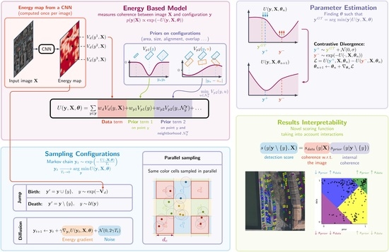
In this paper, we propose the incorporation of interaction models into object-detection methods while taking advantage of the capabilities of deep convolutional neural networks. Satellite images are inherently imperfect due to atmospheric disturbances, partial occlusions, and limited spatial resolution. To compensate for this lack of visual information, it becomes essential to incorporate prior knowledge about the layout of objects of interest.
Instead of increasing the complexity of the model by adding, for example, Transformers to a deep CNN architecture, we propose in this paper to combine CNN pattern extraction with the Point Process approach. The starting point of this approach is to use the output of a CNN as the data term for a Point Process model (
Section 2.3). From the latter, we derive more efficient sampling methods for the Point Process that do not rely on application-specific heuristics (
Section 2.4). Then, we propose to bridge the gap in terms of parameter estimation using modern learning techniques inspired by Energy-Based Models (
Section 2.5). Ultimately, we introduce a novel scoring function that takes into account object interaction in measuring the confidence in the detections and enables explainable results (
Section 2.6). The final part presents quantitative and qualitative results on optical satellite data (
Section 3).
2. Materials and Methods
In this paper, we propose an object-detection method leveraging CNN-extracted information within a Point Process framework that models object interactions. First, we introduce the foundations for the Point Process on which our model is built, then detail the energy model, along with its sampling and parameter estimation method. We also propose a novel scoring method to evaluate the confidence in the output while considering the interactions and providing explainable results.
2.1. Materials: Datasets
To train the CNN and infer the model parameters
, we compile
, a dataset of vehicles in remote-sensing images with
m per pixel resolution, from the DOTA dataset [
25]. This dataset
is built by sub-sampling images from DOTA to the desired spatial resolution and keeping only
small-vehicle and
large-vehicle classes. The data consists of images from satellite or aerial sources of urban or countryside scenes with variable densities of objects (from isolated cars on country roads to dense parking lots). The images are labeled with sets of oriented rectangles for the objects of interest. We also compile a noisy version of
:
+
noise, by adding a Gaussian noise on each image (
) to test the resilience of the methods against noise. Moreover, we evaluate models on data provided by ADS. These aerial data are sub-sampled to the desired resolution, emulating the above-mentioned satellite characteristics. This dataset is unlabeled; thus, it will only serve to evaluate the models qualitatively and was not used for training.
2.2. Point Process for Object Detection
Point Processes model configurations of points (a finite non-ordered set of elements of ) as realizations of a random variable in the set of all possible configurations (with an arbitrary amount of points). Space corresponds to the image space, and to the mark space. The marks can be any random variable that describes the point beyond its location, from the radius of a circle to a discrete categorization of the object. Additionally, we denote the number of points in the configuration and the set of all n points configurations.
As we look to detect vehicles, we model points as rectangles described by the following marks: width
, length
, and angle
as shown in
Figure 1 (with the mark space defined as
).
A Point Process
is described by its density
h relative to the uniform Point Process [
17]. The model of selection and interaction of points derives from an energy
U, through a Gibbs density:
where
is the image,
the parameters of the model, and
Z is a normalizing constant. This constant is intractable due to the non-fixed dimension of
. However, it can be shown that
Z exists (The existence and finiteness of
Z are sufficient as the following computations will consider ratios of
h; thus
Z will cancel out.) and thus
h is properly defined as the energy per point is bounded (see
Appendix A.2). In short, the energy function
U measures the compatibility of the configuration
with the image
; the lower the energy, the higher the compatibility (see Energy-Based Models [
26]). It follows that the most compatible output
minimizes the energy
U (i.e., maximizes the density
h).
2.2.1. Markovian Point Process
For most applications [
18,
20,
21,
23], the physical constraints of the system that is being modeled imply that the marginal density of a point
should only depend on a neighborhood around it (e.g., vehicles only align with others within a limited distance). This property is formalized through the Markovianity of the Point Process.
Definition 1. Point Process is a Markov Point Process under the symmetric and reflexive relation∼if and only if, for every configuration such that [17]: For every point , only depends on u and its neighbors according to ∼ (i.e., ).
Theorem 1. For a Point Process derived from the energy:where is the set of neighbors of y for relation ∼. Then, the Point Process is Markovian for relation with . In short, if the energy of a point y depends on its neighbors within a distance of , the Point Process is Markovian for a distance . The Markovianity will prove useful to simplify the sampling procedure and run it in parallel over the whole image.
2.2.2. Papangelou Conditional Intensity
The reference Poisson Point Process has an intensity
that is either constant or depends on the location (For any compact
,
if
is constant.). The density in (
1) implies the intensity is now a function of the location and neighborhood of a point:
Definition 2. The Papangelou conditional intensity [17] associated with a Point Process , is defined as:i.e., the infinitesimal probability of finding a point in region around, given the configurationoutside (
i.e., ). When , the Papangelou conditional intensity can be computed from the energy function U as: 2.3. Energy-Based Model
The energy formulation of the Point Process allows the compositing of several simple point behaviors into one model. We illustrate the composition of several simple point distributions through the addition of energy terms in
Figure 2: There, we show that the point distribution in (
Figure 2d) can be obtained by simply adding the energies used to produce
Figure 2b,c.
When performing object detection, the image provides information about the location and properties of objects (e.g., location-based energy as in
Figure 2b), while prior knowledge of the objects of interest complements this information (e.g., a repulsion term as in
Figure 2c); the composability of the energy model allows the factoring in of both pieces of information into a single model (as in the composition of
Figure 2d).
More specifically: For every point
we compute a set of energy terms
,
and combine those—per point—as a weighted sum [
20,
21,
23]:
with
is the energy contribution of a single object
y. Energy terms can be grouped into two categories:
Prior terms (of the form ) that only depend on y and its neighborhood ; they measure the coherence of the configuration itself considering the known properties of the objects of interest (e.g., objects do not overlap).
Data terms () are a function of y and the image (also referred to as observation in remote sensing); these terms measure the correspondence of the points with the image.
The weights
w are part of the parameters
that will need to be set before inference on any unseen image. We discuss the estimation of parameters
in
Section 2.5.
In the rest of this section, we define the multiple energy terms : First, the data terms, then the prior terms. Contrary to previous Point Process (PP) approaches, we do not rely on contrast measures but rather on data terms pulled from the output of a CNN: this allows for more reliable measures and faster computation. Moreover, this new model formulation opens up new improvements in sampling the energy model and estimating its parameters.
2.3.1. Data Terms from a CNN
Classical likelihood measurements [
18,
20,
23] are based on contrast measures that are crafted to fit each application. Moreover, these measures rely heavily on the high contrast between objects and their background, along with limited background diversity. We illustrate the limitations of those in
Section 3.1.
On the other hand, CNN models have shown to be very efficient at extracting features from images for object detection and classification. In the following section, we will show how to interpret a CNN-based object detector output to obtain a scalar energy that measures the fitness of a configuration against an image. It allows us to go past the contrast measure design by utilizing a pre-trained CNN output.
Position Likelihood Term
CNN-based object-detection methods such as [
7,
8,
27] make use of a heatmap to find object centers. This object center probability map is obtained by passing the image
of shape
(here with 3 color channels) into a fully convolutional model such as Unet [
28]. It outputs a tensor
, from which a probability-like measure of an object center at coordinates
is obtained as
where
is the sigmoid function, and
the value of map
at coordinates
.
We propose to reinterpret this output as the position energy as follows:
with
a scalar threshold, allowing the movement of the inflection point of the Softplus function
.
Mark Likelihood Term
To compute the energy associated with marks, we discretize each mark
(
in the case of a Point Process (PP) of rectangles), into
classes (or value bins) in the range
. We define the integer class of a value
v for mark
as:
with
being the corresponding integer class.
Now, supposing we have a model trained to classify the mark of an object at a given position
, such a model will produce a probability estimate of mark
to be in class
, from model output
as:
As in [
29], we can reinterpret the model output into a potential, giving:
As the CNN outputs a tensor
of shape
, we obtain vector
by sampling tensor
at location
, as illustrated in
Figure 3a. Vector
gives an estimate of the probability of each class
c once passed through a Softmax (as given by (
8)); We illustrate this with the histogram, on top of
in
Figure 3a. The value of
is then obtained by applying the formula in (
9) over vector
(as illustrated on the right-hand side of
Figure 3).
Interpolation
The energies described in (
6) and (
9) are defined over integer coordinates in
and integer classes in
. However, points
y in the configuration
have real-valued locations
as is for marks in
. Thus, we propose interpolating values between exact pixel locations. For (
9) we now have:
The above has two benefits: first, (
10) defines the energy for continuous values of the marks using bilinear interpolation, thus ensuring Lipschitz continuity of the energy. Second, we can pre-compute (11) once for a given image, making the mark energy computation a simple value lookup and interpolation for each point. In practice, we proceed as illustrated in
Figure 3b, where a function is applied to the CNN output
to obtain
, which is stored in memory. The interpolation gives
for any continuous position and mark. This pre-computation is quite fast, as it is defined as an operation over a tensor, which is implicitly parallelized by tensor computation libraries such as PyTorch [
30]. The same holds for the position term (
6).
2.3.2. Energy Priors
The total energy model encompasses several priors as energies, which allows regularizing configuration against the data terms.
2.3.2.1. Object Priors
These are functions of the current point
y only. For
:
with
and
, and
,
being, respectively, the target value and the standard deviation. These two are illustrated in the first line of
Figure 4.
For our objects of interest, we find two modes in the distribution of areas and ratios: Cars and trucks. To make sure to only favor these two modes and not objects with the area of a truck and ratio of a car, we introduce a joint area and ratio prior:
2.3.2.2. Interaction Priors
The following priors depend on the neighborhood of the point
y. The term in (
14) penalizes overlapping objects (with
the overlap threshold), (15) favors aligned objects (
favors parallel objects, while
prefers perpendicular objects), (16) and (17) are, respectively, repulsive and attractive priors. Finally, (18) allows the adjustment of the energy of neighborless points. Some of these priors are illustrated in
Figure 4.
where
for
. Note we introduced a few parameters
, these will have to be either set by trial and error or through the parameter estimation method presented in
Section 2.5.
2.3.3. Model Pipeline
We summarize the implementation of the overall energy model in
Figure 5. As is, our architecture has the following advantages:
2.4. Sampling Configurations from the Energy Model
For a given energy model
U (supposing parameters
are set), we aim at sampling configurations that follow the Gibbs density defined in (
1). This will allow us to find the most compatible configuration
for any image
, i.e.,:
As the space
in which we are trying to minimize the energy is not of fixed density, we must resort to an adapted sampling method such as Reversible Jump Monte Carlo Markov Chain (RJMCMC) [
31]. While this method ensures proper sampling of the desired law, it often requires some application-specific adaptations to improve sampling time and efficiency (e.g., [
20,
23]).
Here, we propose to use the already computed energy maps and to add new points in relevant areas and to focus on the parallel sampling of the algorithm. Moreover, the implementation of our energy model allows us to leverage automatic gradient computation to implement diffusion dynamics and explore at a fixed number of points (i.e., within ) guided by the whole energy model.
2.4.1. Birth Maps for Efficient Point Proposals
At their core, both RJMCMC [
31] (an adaptation of the Metropolis-Hastings algorithm [
32] to variable dimension problems) and Jump Diffusion [
33] make use of Birth and Death moves to build a Markov chain
of stationary density
where
is a temperature parameter that decreases towards zero (i.e., Simulated Annealing) (Convergence is proven for a logarithmic temperature decrease, here (and in the literature) we approximate it with a geometric decrease at it is faster [
17]). That way, the chain converges towards the global minimum energy. Proposed Birth (addition of points to the current
) and Deaths (removal of points) are accepted or rejected given an acceptance ratio that depends on the energy change induced by the respective addition or removal of points (for more details see [
31,
34]).
The simplest birth move is to propose new points uniformly in
. However, this proves highly inefficient as the density of objects in the image varies a lot. Ideally, the birth move would propose a new point
u to the current configuration
, sampled with the marginal density
as is carried out within Gibbs sampling (maximizing the chance for the point addition to be accepted). Knowing that
, we could compute the marginal density using energy change induced by adding the point. However, this cannot easily be computed because of the interaction terms. Thus, we propose to approximate it by only considering the data terms (i.e., bypassing the energy change on prior terms):
From this, we define the density
d to sample a new point
u:
with
and
the pre-computed position and marks energy maps. Since both are defined as tensors with a finite number of elements, the normalizing constant
in (
21) can be computed over this discretized space of pixels and mark classes.
This allows for efficient sampling of new points, without any application-specific heuristics, by taking into account a truncated version of the energy model U that can be normalized easily.
2.4.2. Focused Parallel Sampling
In its canonical implementation, the RJMCMC algorithm operates sequentially over the points in the image—It may only add/remove/transform one point at a time —, which increases simulation time linearly with the number of objects. With parallelization, we aim to take advantage of the spatial Markovianity of the Point Process, as Theorem 1 states that moves further than apart are independent.
As in [
35], we split the image into square cells of size
that are each assigned one set
s (each set corresponding to one color in
Figure 6). These sets are referred to as mic-sets in [
35] for Mutually Independent Cells. Set size
is chosen as
(
is the maximum point translation distance, introduced in the next Section), so that moves in cells of one set (or color) have independent acceptance ratios: i.e., those moves can be performed in any sequential order –thus in parallel—without any change in the probability of acceptance. In practice, we have
(
,
).
We aim at leveraging the birth map stemming from the pre-computed energy maps
and
to focus the sampling on parts of the image where the density of objects is high. Contrary to [
35], we do not use a quadtree structure of cells, but rather a regular grid of
sized cells. In order to achieve an efficient sampling of cells (i.e., avoiding spending time in cells with no evidence of objects), weights are assigned to each cell to focus the sampling on the relevant ones. The sampling procedure goes as follows:
pick a move type (Birth, Death, or Diffusion),
pick one set s with probability ,
keep each cell in set s with probability
for every cell c in set s run move restricted to c (Birth density becomes )
The process of cell selection (step 3) allows for limiting the number of cells processed at once on big images, hence limiting the computational cost and focusing the sampling on areas with high object density. We pick the following densities:
denoting (by extension)
and
the density
d integrated over all cells of set
s and cell
c, respectively. In practice, parameter
ensures new points are sampled over the whole image with density
d; higher values of
allow for more parallel cells to be sampled each step at the cost of straying away from density
d.
2.4.3. Jump Diffusion: Leveraging Gradients
The canonical RJMCMC algorithm also uses local transform moves to explore
at a fixed number of points, picking one point to translate, rotate, and scale at random in
. This is wildly inefficient as it does not consider the energy function
U it is trying to minimize. Instead, we propose to use the energy gradient to explore the space more efficiently. This is the idea behind stochastic diffusion (or Langevin) dynamics [
36,
37]. If
and
denote, respectively, the configuration and temperature at time
t, then the configuration for the next step of the Markov chain is given by
, with step size
:
At high temperatures, the Brownian motion from
ensures an exploration of space. At low temperatures, the Brownian motion is negligible, and the diffusion performs as a gradient descent. This allows fine-tuning the configuration at low temperatures while considering the whole energy model (contrary to the truncated energy used for birth maps in
Section 2.4.1).
The diffusion alone allows for the exploration of space
locally around
at a fixed dimension (fixed number of points). To explore (or
jump) across dimensions, we make use of the Birth and Death moves as defined previously (see
Section 2.4.1).
In practice, as parallelization requires some maximum displacement on points (see
Section 2.4.2), the step
from
to
is clipped; for each point
updated to
, we bound the
i and
j components by
(i.e.,
, and similarly for
j).
2.4.4. Resulting Sampling Method
The resulting sampling method is outlined in Algorithm 1. The method requires the following inputs:
: initial configuration;
: image;
: energy model parameters;
: initial temperature;
: number of samples;
: temperature decay rate.
Here, we denote by
the restriction of configuration
to cells
c. Please note that to compute
U for iteration of the loop on
t, and the energy maps
,
are only computed once as stated in
Section 2.3.3.
| Algorithm 1: Sampling method. |
- Input
- 1:
fordo - 2:
Pick diffusion with probability , else jump - 3:
Pick mic-set s with probability - 4:
Keep each c in s with probability to make - 5:
unvisited cells will keep the previous state - 6:
for all - 7:
if diffusion then - 8:
- 9:
- 10:
- 11:
else - 12:
with probability else pick birth or death - 13:
remove a point at random or add one using the birth map - 14:
compute Green ratio - 15:
with probability - 16:
end if - 17:
end for - 18:
decrease temperature - 19:
end for - Output:
|
The above implements the sampling improvements described previously, namely:
sampling new points using the birth map (line 13),
sampling in parallel over the whole image (line 6), in practice using tensor batch dimensions,
using the energy gradient to perform Diffusion (line 9).
2.5. Estimating Model Parameters
In this section, we estimate the parameters
, so that, for each image
, the associated ground truth configuration
matches the most compatible configuration, i.e.:
Previous PP approaches for object detection often relied on trial-and-error parameter estimation or used linear programming [
23,
38]. The latter method would generate a set of constraints (These constraints can be seen as a local reformulation of global constraint (
26).)
where
wrong configurations are generated by applying strong perturbations on the ground truth configuration
. However, this only estimates the weights
and is prone to over-constraining when the ground truth is noisy or when considering too many constraints. Moreover, this method requires designing the procedure to generate the configurations
, which we find has a great effect on the estimated parameters.
2.5.1. Maximum Likelihood Learning
To tackle the above limitations, we turn towards the Energy-Based Model (EBM) literature for new parameter estimation methods. The authors in [
26] propose to learn EBM parameters by maximizing the likelihood for the data
:
The negative log-likelihood is then given, for parameters
at step
n, as:
with
an inverse temperature parameter (from the Gibbs distribution) that does not affect the position of the minimum [
26]. The gradient of
on
is shown to be
where
.
While the integral
remains intractable, it can be approximated through Monte Carlo sampling, where
are drawn from the law defined by
, which yields:
2.5.2. Contrastive Divergence
The authors in [
39,
40] propose to use a single sample in their Contrastive Divergence (CD) method. This method also uses a few simulation steps for the Monte Carlo Markov chain (MCMC) to generate
, starting from the desired answer
.
The general idea is to generate
contrastive samples that follow the density derived from
at step
n of the optimization. Then we proceed to update
to
, by gradient descent, to minimize the energy of the
valid sample , while maximizing the energy of the
contrastive sample (see
Figure 7). Alternatively, we can augment the data and use
positive samples to replace
as in [
41]. In the case of imperfect GT, this models the uncertainty over the labels while providing some data augmentation.
The loss to minimize is then:
with
the weight of regularization term
. We introduce the regularization term to avoid an explosion of the per-point energy
. To ensure a sparse weighting of energies (i.e., minimize the number of non-zero weights
) we can introduce a new regularization term as an
norm on the vectors of weights [
42]:
The broad strokes of the estimation procedure for parameters
are as follows:
Pick a pair from data .
Generate positive sample .
Generate negative sample .
Compute the loss
(see (
31)).
Update
to
according to the gradient
, with the Stochastic Gradient Descent (SGD) method [
43], as illustrated in
Figure 7.
Loop back to step 1 until convergence.
2.5.3. Replay Buffer
As sampling contrastive samples
can be time-consuming, we use the replay buffer introduced by [
41]. The replay buffer saves Markov chain results at the current optimization step to use for initialization in the next steps, thus saving computing time. This allows for reducing the long simulation time necessary to pass the burn-in period of the Markov Chain [
44] and obtain samples
. We use a sample from the law derived from
to initialize the chain that samples the law derived from
. The use of the replay buffer within one step
n of the optimization loop goes as follows:
With probability set configuration as a value of the replay buffer picked at random. With probability (or if the buffer is empty) set configuration as a random configuration in .
Run the Markov Chain to simulate model of energy .
Use as a negative sample for the loss computation and update of to .
Update buffer .
This buffer allows running longer chains across epochs (i.e., obtaining higher-quality samples) while maintaining a low computational cost.
2.5.4. Parameters Estimation Algorithm
The final parameter estimation algorithm is as follows:
At line 4 we select a temperature at which to run the Markov chain to sample the negative configuration (, , ); higher temperatures allow sample diversity, while lower ones seek points of minimal energy within the current energy model. Scaling computed at line 6 allows rescaling the energy to a unit variance model in order to ensure consistency in sample diversity for a set temperature. It is computed over 1000 samples . Finally, for each temperature and image , we set a specific buffer . The parameter K is the number of steps the Markov chain runs for every gradient descent step. In practice, we set so that the number of iterations scales with the number of pixels in a cell.
Algorithm 2 we propose above provides a single procedure to estimate all parameters in
rather than only the weights
as done previously with linear programming in [
23,
38]. On top of avoiding over-constraining by having no hard constraints, our method also removes the need to design a procedure to sample configurations
as those are sampled from the current energy model
. Finally, the replay buffer allows for qualitative samples while maintaining a limited computational burden.
| Algorithm 2: Contrastive Divergence parameters estimation. |
- 1:
- 2:
while not converged do - 3:
for all in - 4:
select temperature to sample negative config. - 5:
with probability , else retrieve relevant buffer - 6:
compute energy scale - 7:
see Algorithm 1 - 8:
- 9:
- 10:
Update with using SGD - 11:
update the buffer - 12:
- 13:
end for - 14:
end while
|
2.6. Papangelou Intensity as a Confidence Score
Classical CNN-based object-detection models for object detection (such as [
8,
45,
46]) yield a confidence score
for each proposed object
y in the image. This confidence score is often interpreted, for each detection, as proportional to the probability of proposed element
y to be a true positive,
. Applying a score (or confidence) threshold
gives a set of detections for which metrics such as precision and recall can be computed by matching the detections with the ground truth. This allows adapting the threshold according to the need for the application; i.e., some applications may require low false positives (high precision) while others require fewer missed detections (high recall). To assess the performance independently of the threshold selection, the Average Precision (AP) metric sums up the performance of a model as the area under the Precision-Recall curve.
Previous Point Process approaches [
18,
47,
48] only compute simple metrics such as precision, recall, or F1 score for the configuration given by the sampling procedure, as no score is associated with each object detection.
2.6.1. Papangelou Intensity as Score
With our PP approach, we propose to introduce a scoring function, first to filter the detections given a confidence threshold and second to be able to compare our method to others using the widely used AP metric. Within the PP framework, the probability of one proposed point being an object of interest depends on the rest of the inferred configuration
; thus the scoring function reflects it:
. From (
3), we have that the Papangelou conditional intensity is proportional to the probability of finding a point
in a small neighborhood
knowing the rest of the configuration
. We propose to use the Papangelou conditional intensity as a score:
2.6.2. Pruning Sequence
However, the dependency of the score on the current configuration yields a complication while computing the AP: when applying a threshold to prune the configuration into , for any , the score may differ from . With a score of the form that only depends on y and the image —such as those from classical CNN models—the score from one object after pruning is unchanged.
In the PP case, we compute the scores by sequentially removing the lowest scoring point until none is left; i.e., we build a sequence of configurations
, with
, for
:
Equation (
34) provides a pruning order
of points in
. This ordering allows plotting the precision and recall curve. Indeed, to trace a Precision-Recall curve, one only requires the sequence of
pairs, which are obtained by sequentially pruning the lowest scoring points. Equation (35) provides a score for each point
.
2.6.3. Contrastive Divergence Loss and Papangelou Intensity
On the one hand, the energy model is trained by minimizing the loss function in (
31) derived from the likelihood maximization of the parameters regarding the annotated data. On the other, we evaluate the performance of the inferred configuration with the scoring method in (35) sourced from the Papangelou intensity. Here, we show that while the two are derived differently, the minimization of the loss function leads to good properties on the score function.
Here, we consider a simplified loss with only the two energy terms (as
). Denoting the energy change induced by the move from configuration
to
as
, we have:
Similarly, the Papangelou intensity can be rewritten as such:
Single Point Addition
Thus, for a simple negative sample
in which we add a non-valid point
u to
, we have:
This leads to the expected behavior: minimizing the loss
leads to minimizing the score of non-valid point
u. The same stands for the removal of a valid point
and maximizing its score.
Arbitrary Sequence of Moves
This is also valid for the generic case where
is generated from an arbitrary sequence of additions or removal of points (A translation/rotation/scaling can be viewed as removal and addition.) from
. This defines a sequence
of
n configurations as:
with
,
, and
elements of either
or
. Without loss of generality, we can reorder the sequence to match the pruning order defined in (
34). The energy change for one move is given as:
As we have (by definition)
, the loss is given as:
By ordering the
to match the pruning order in (
34) each
can be matched to their respective score:
(
41)(a) corresponds to non-valid points added to
, their score is minimized as the loss is decreased;
(
41)(b) corresponds to valid points removed from
. Their score is increased as the loss is minimized.
With this, we showed that minimization of the loss at a configuration level leads to the expected results on object scores.
While this score function allows taking into account the interaction between objects that the PP model introduces, the decomposable nature of the PP (see (
5)) allows for the interpretability of the results as demonstrated in
Section 3.4.
2.7. Method Summary
In this section, we proposed a model for object detection that combines CNN architectures with a Point Process (PP) framework. Before applying our approach to real data, we shall summarize its function here. Considering configurations of objects
, image
, and parameters
, we look to build an energy model
such that the minimum energy point of it corresponds to the ground truth configuration for that image
. As such, we build
U to be a combination of multiple energy terms (Equation (
5)), with prior terms that encode the interaction model of our objects (where high energies repel unwanted configurations and lower ones favor others), and data terms that we build from the features from a CNN (
Section 2.3.1). We refer the reader to
Figure 5 for an overall view of the model pipeline. Within this framework, we can combine the information from the image with the prior knowledge of the configurations.
To estimate the parameters
, we propose to use Contrastive Divergence. In short, we initialize the parameters at random and alternate between sampling low-energy configurations with the current parameters—that are nowhere close to the ground truth at the beginning of the procedure—and updating the parameters to increase the energy of these samples while maintaining low energy for the ground truth (
Section 2.5). This allows us to estimate any differentiable parameters in the model, while previous methods would often become over-constrained and could only estimate linear parameters.
Now, given parameters
are set, we want to estimate the configuration of an unseen image
. This is achieved by sampling the configuration
that minimizes the energy through a Jump Diffusion mechanism. Alternatively, proposing to add or remove points in the configuration guided by the energy maps the CNN provides (
Section 2.4.1) and lowering the energy locally at a fixed number of points with gradient descent (
Section 2.4.3). The latter can be applied in parallel over the image while focusing on patches of the image with higher expected object density (
Section 2.4.2).
Lastly, we propose a metric based on the Papangelou intensity that allows us to compare our approach to others and takes into account the object interactions in the likelihood of detection (
Section 2.6).
4. Discussion
4.1. Quantitative and Qualitative Results
In
Figure 10, we observe that despite noisy ground truth labels—a potential cause for over-constraining issues when using linear programming (see
Section 2.5)—our models infer more regular configurations that align better with the physical constraints of the objects of interest. Sample 1 in
Figure 10 BBA-Vec. struggles to properly align and detect all the objects. In sample 2, model YOLOV5-OBB shows patches of objects with no overlap regularization. Meanwhile, our model outputs regularized configurations even in these dense areas.
Figure 10 (line 3) and
Figure 11 showcase the robustness of our PP-based models when tested on noisy data or areas of limited information, such as shaded areas. The inference results on the
ADS dataset, obtained with models trained on the
training set, highlight the model’s ability to generalize to unseen, albeit similar, data.
Comparison between
and
against CNN-LocalMax. in
Figure 10 and
Table 3 reveals the improvement brought by the PP-based approach, as the performance of the CNN alone (CNN-LocalMax.) falls short of our proposed method especially when confronted with noisy data.
Lastly, the comparable performances of and , both qualitatively and quantitatively, highlight the efficacy of the CD method in inferring model parameters. This approach significantly reduces the need for manual parameter tuning (more specifically, prior parameters), where traditional PP methods, such as linear programming, fall short.
4.2. Limitations
Our method, while promising, faces several limitations that warrant consideration. First, the computational complexity involved in sampling a PP can be significant, particularly with dense configurations of objects. To address this, we could explore approximate sampling methods, although this might come at the expense of result accuracy, for instance, by implementing faster annealing techniques or discretizing the state space [
48].
Second, while the model we present is tailored to a specific type of object, the underlying tools are adaptable to various object types. First, the PP framework allows for a wide diversity of objects to be modeled, thanks to the versatility of marks. Moreover, the energy formulation of our model allows for easy integration or removal of interaction models and priors as simple energy functions. For instance, we could incorporate classification as a mark in the Point Process model, utilizing features from the CNN or a prior law based on the geometric features of the objects (e.g., distinguishing trucks from cars based on length).
Lastly, our method relies on annotated data for training. However, energy models offer compositional flexibility; one potential avenue is to train the data terms of the model on annotated images while utilizing synthetic datasets (devoid of visual components) for prior terms training. This approach could help mitigate the reliance on annotated data and improve generalization to diverse scenarios.
5. Conclusions
In this paper, we present a method that integrates interaction models into object-detection algorithms, leveraging deep convolutional neural networks. We address challenges inherent in satellite imagery, such as atmospheric disturbances and limited resolution, by incorporating prior knowledge about object arrangements.
While CNN-based methods excel at pattern extraction, they struggle with learning object-to-object interactions without complex attention mechanisms. Conversely, Point Process methods offer a promising alternative, addressing both object likelihoods and arrangement coherence. However, existing approaches relying on contrast measures have limitations.
Our method combines CNN pattern extraction with the Point Process framework, simplifying contrast measure computations into efficient energy maps. By leveraging pre-computed potential maps, we enhance Point Process sampling methods, improving exploration efficiency within the state space.
We depart from conventional parameter estimation approaches for Point Process methods like linear programming and adopt Contrastive Divergence to estimate energy weights and internal parameters automatically. This improves accuracy and reduces reliance on manual parameter tuning.
To facilitate model comparison, we introduce a novel scoring function based on the Papangelou conditional intensity, providing a more comprehensive evaluation metric that takes into account interactions and allows for the explainability of results thanks to the easy decomposition of the energy model.
Experimental results on diverse datasets demonstrate our method’s effectiveness, particularly in noisy environments. Our model’s ability to generalize to new data showcases its robustness and potential for practical applications.
In conclusion, our method offers a promising approach to object detection, combining the strengths of CNNs with Point Process models. It shows potential for improving accuracy and efficiency in satellite imagery analysis or other applications where the priors are strong: e.g., object tracking (priors on dynamics) or road extraction (geometrical priors).


