

Modeling Land Use Transformations and Flood Hazard on Ibaraki’s Coastal in 2030: A Scenario-Based Approach Amid Population Fluctuations


Abstract
:1. Introduction
2. Materials and Methods
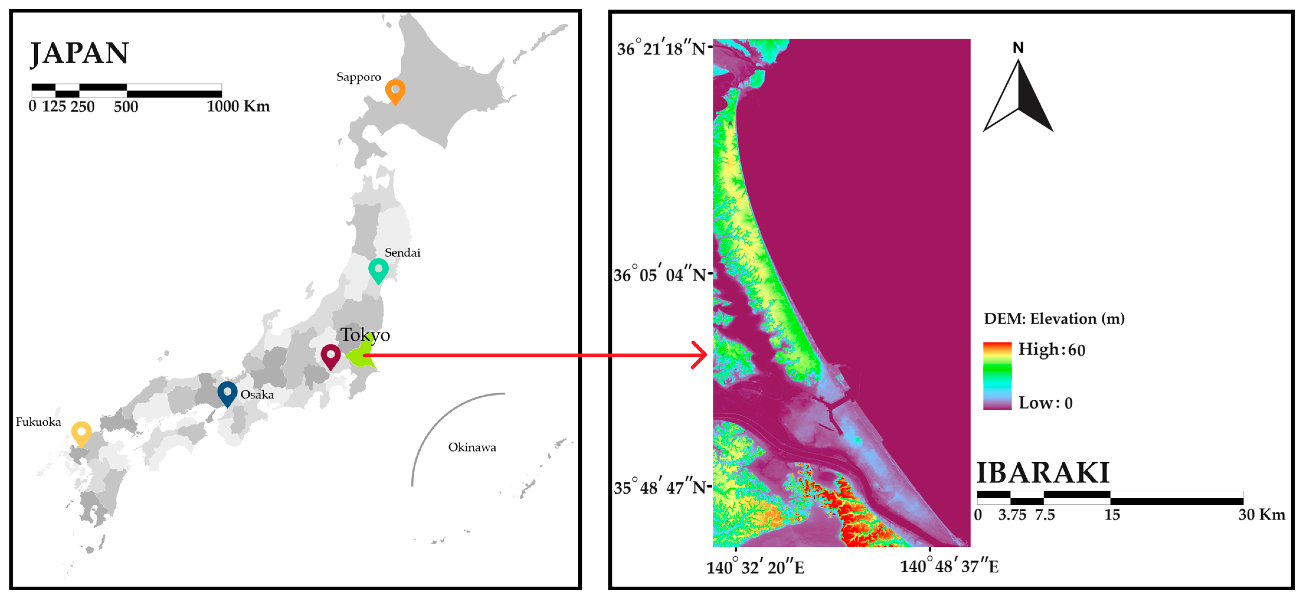
2.1. Study Area
2.2. Datasets
2.3. Methodology
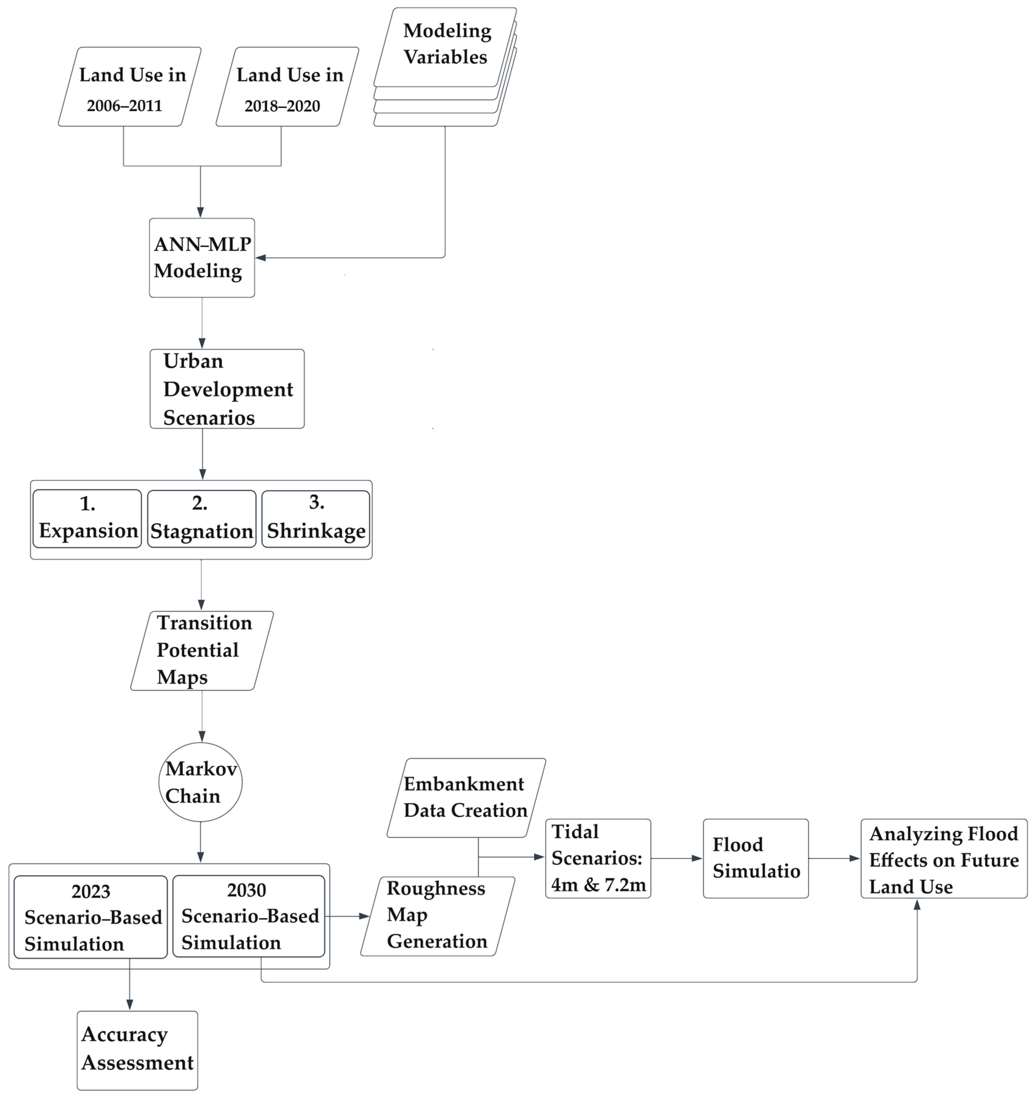
2.3.1. Overview
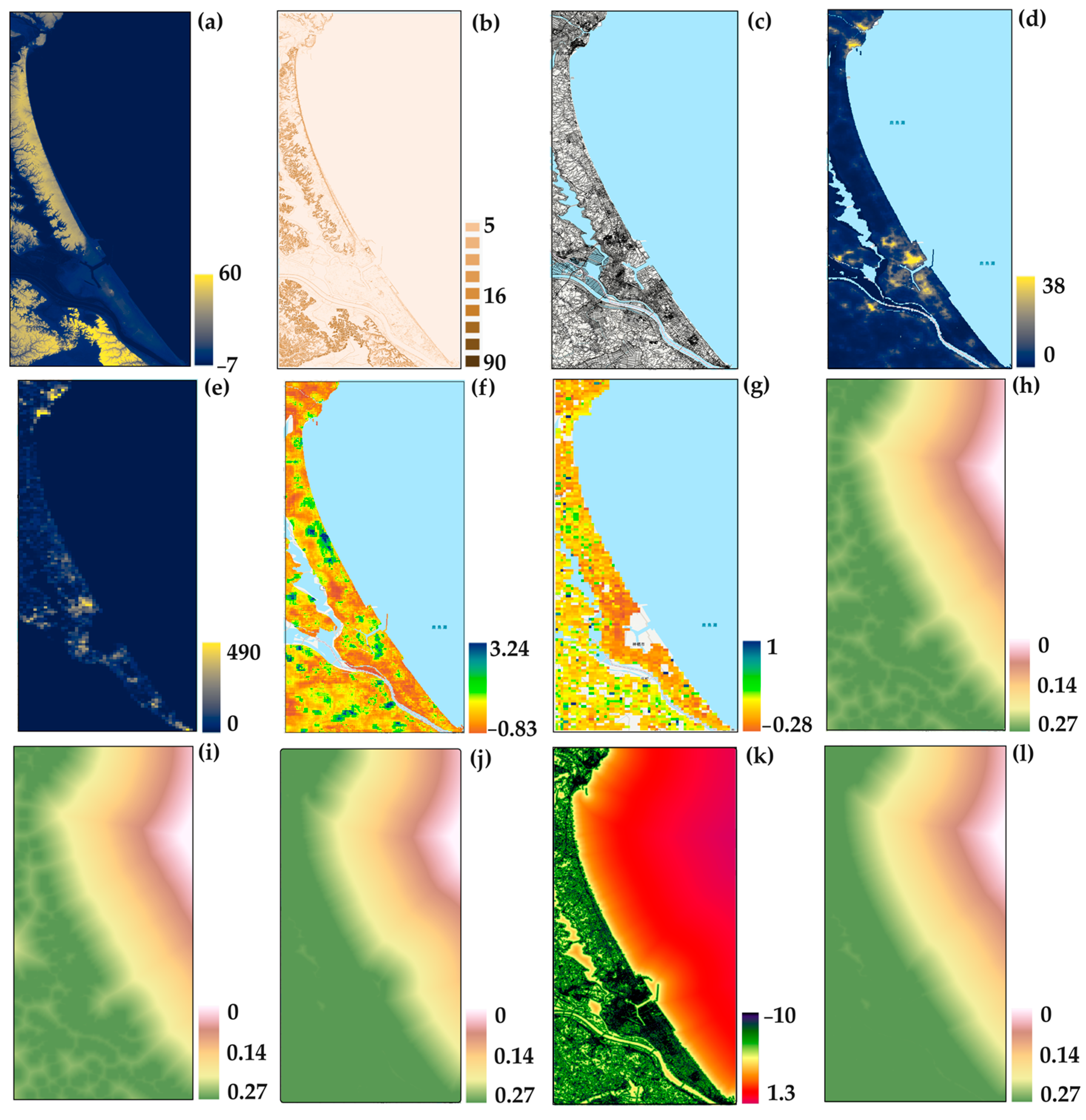
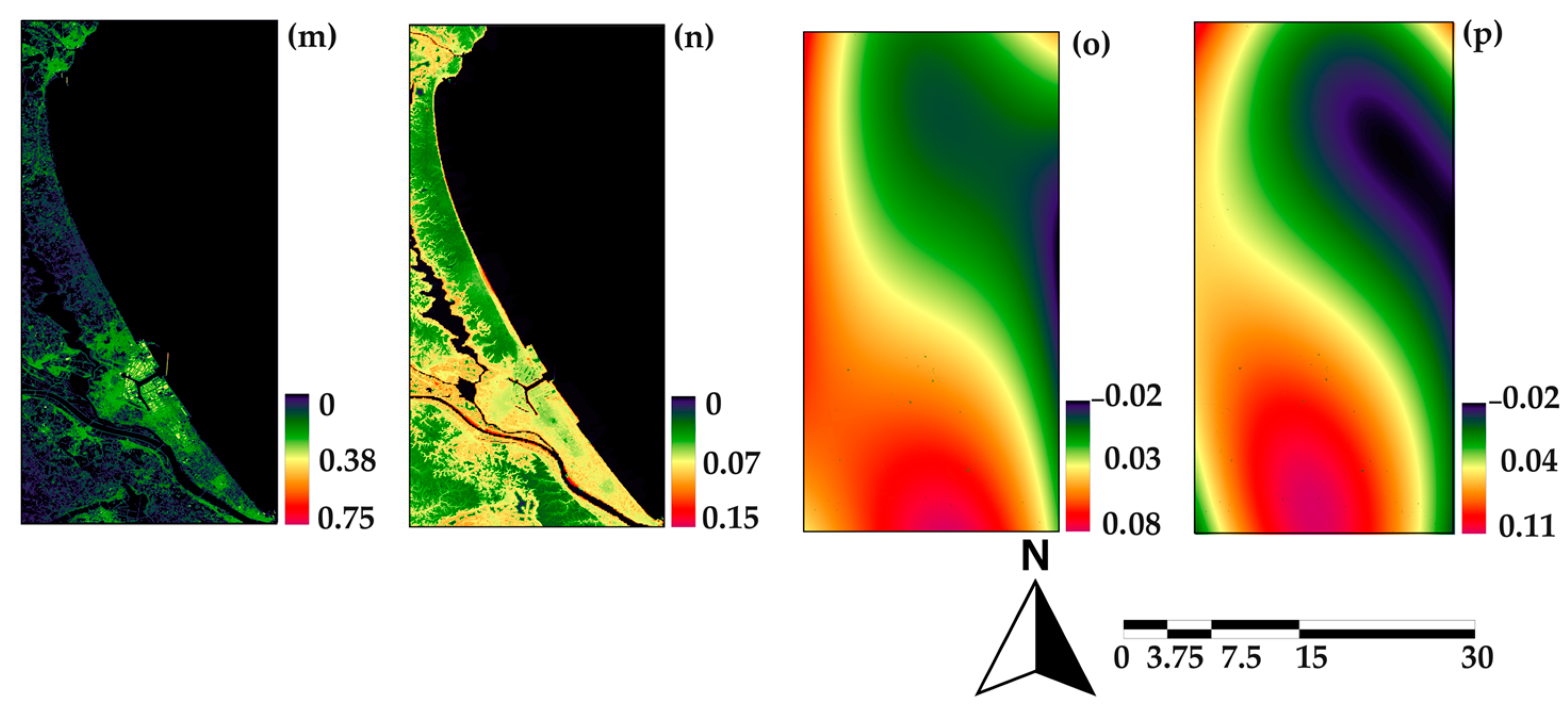
2.3.2. Collection and Creation of Explanatory Variables
2.3.3. Artificial Neural Network-Based Multi-Layer Perceptron and Markov Chain Model
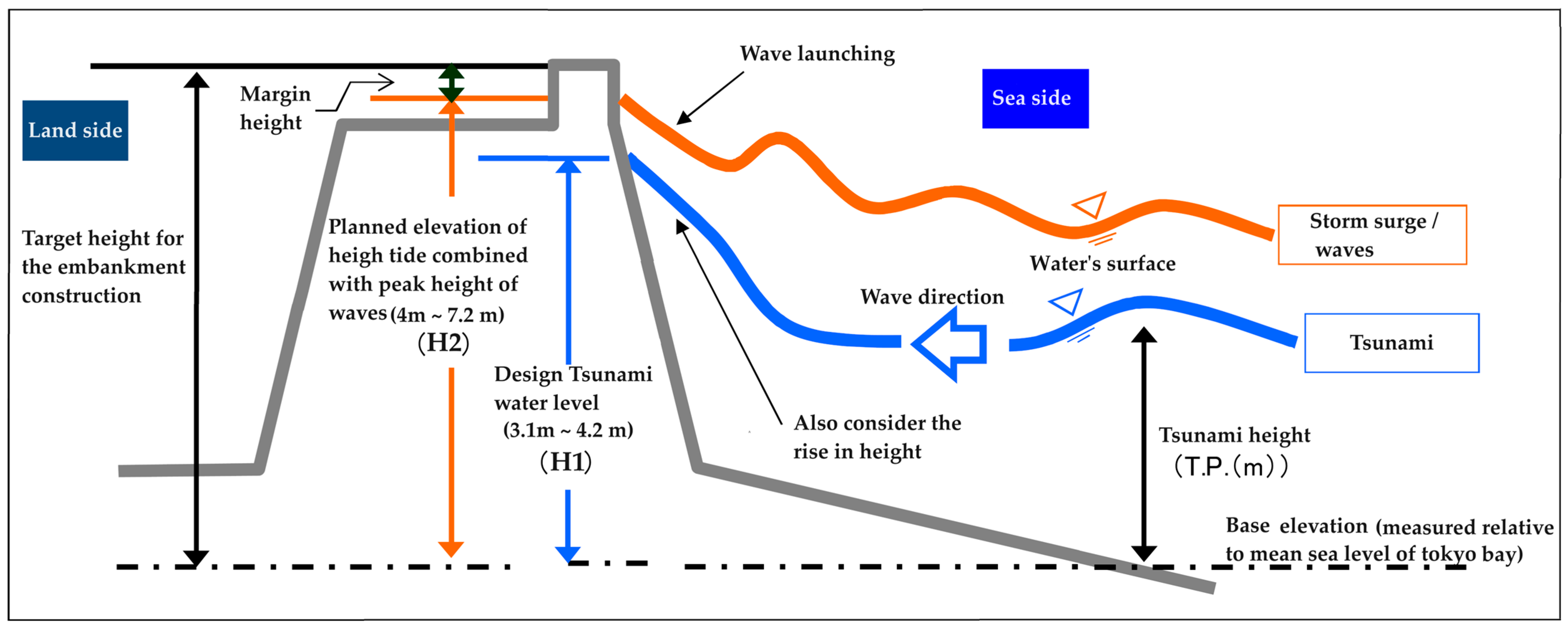
2.3.4. Design for Future High Tide and Wave Crest Scenarios on the Ibaraki Coastline
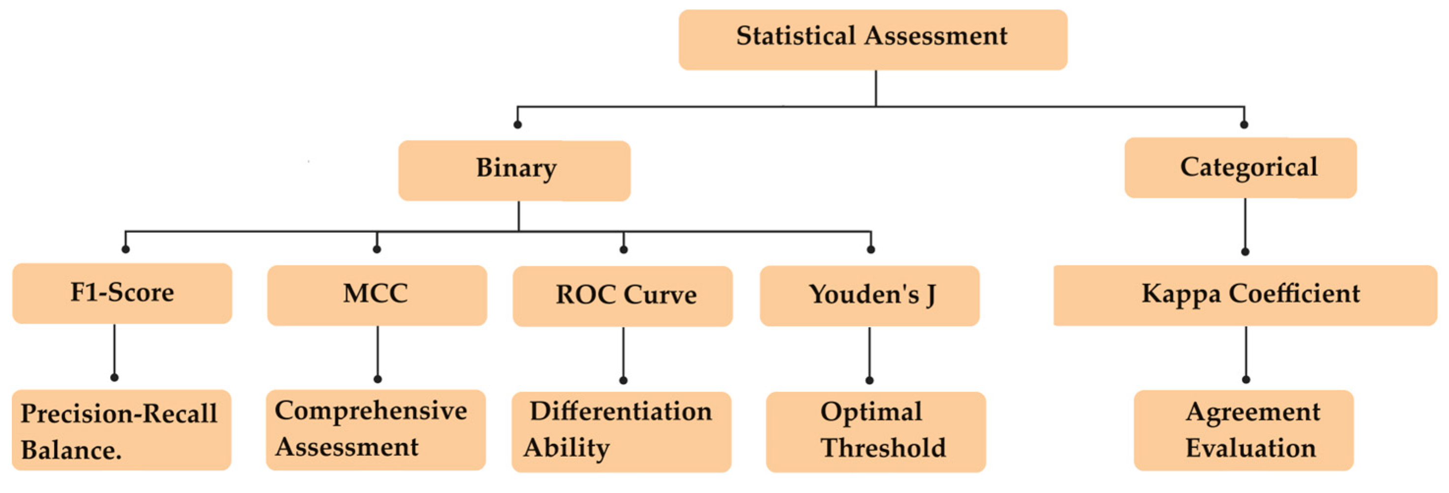
2.3.5. Verification of Projected LULC Maps for Different Scenarios
3. Results
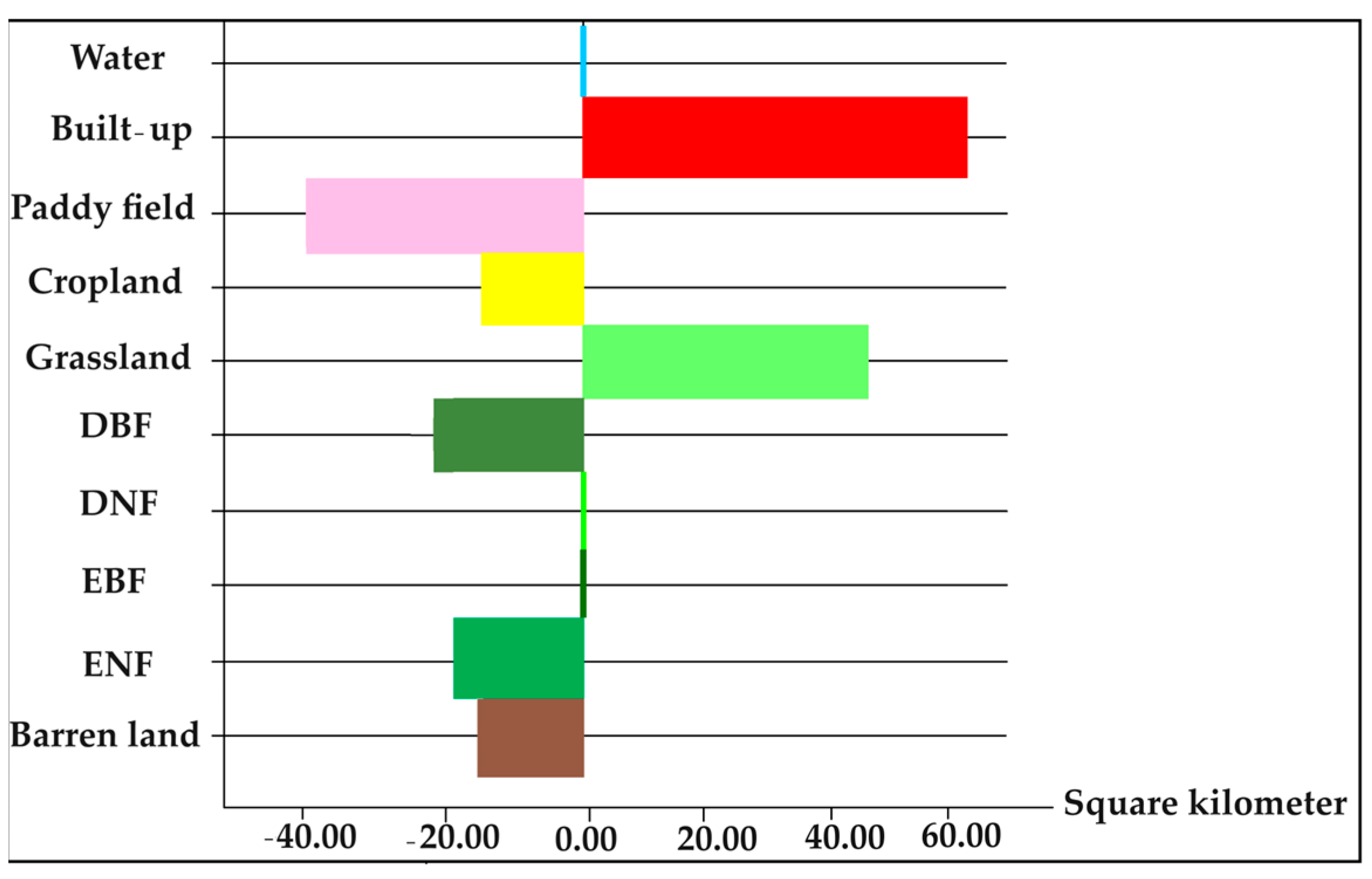
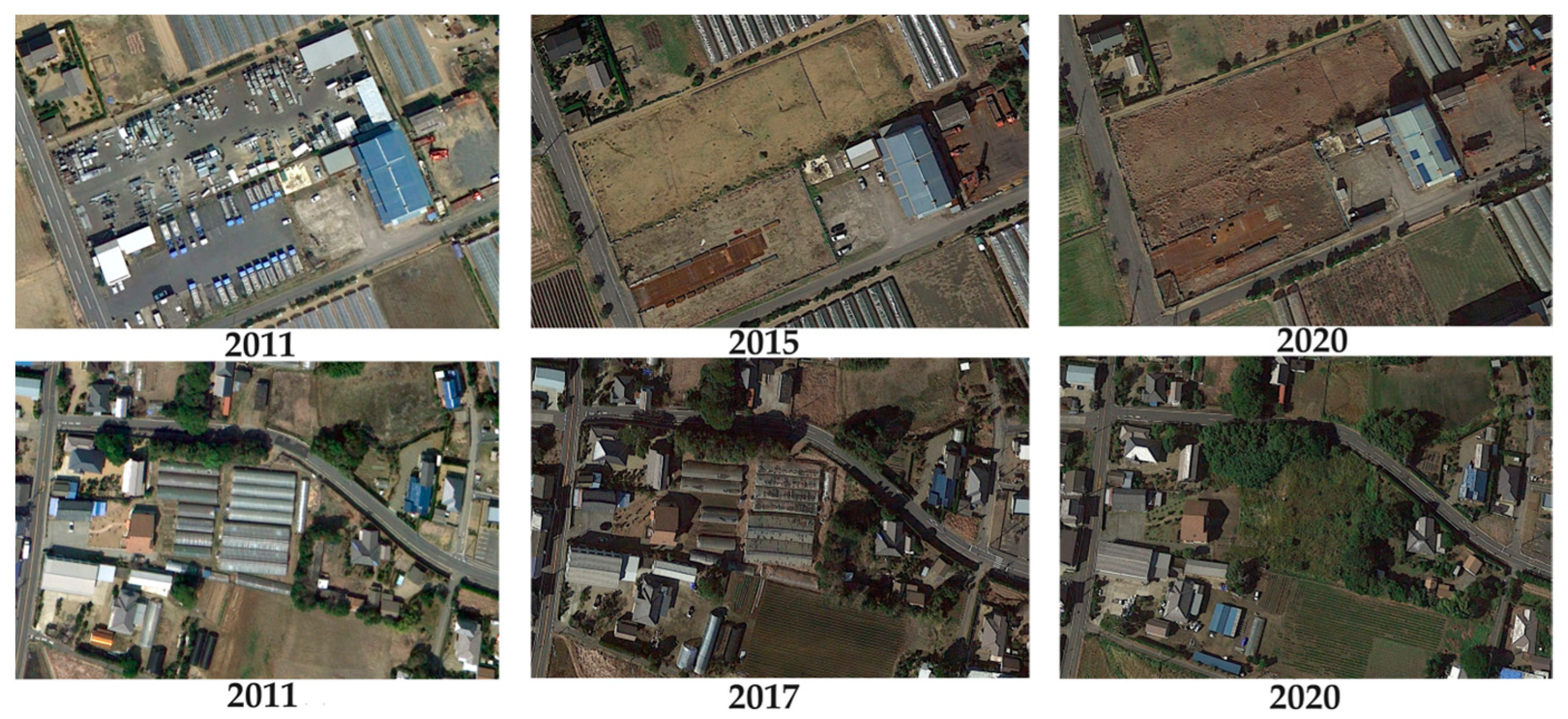
3.1. Comparative Analysis of Land Use: Initial Map (2006–2011) versus Second Map (2018–2020)
3.2. Contribution of Each Explanatory Variables in ANN-MLP
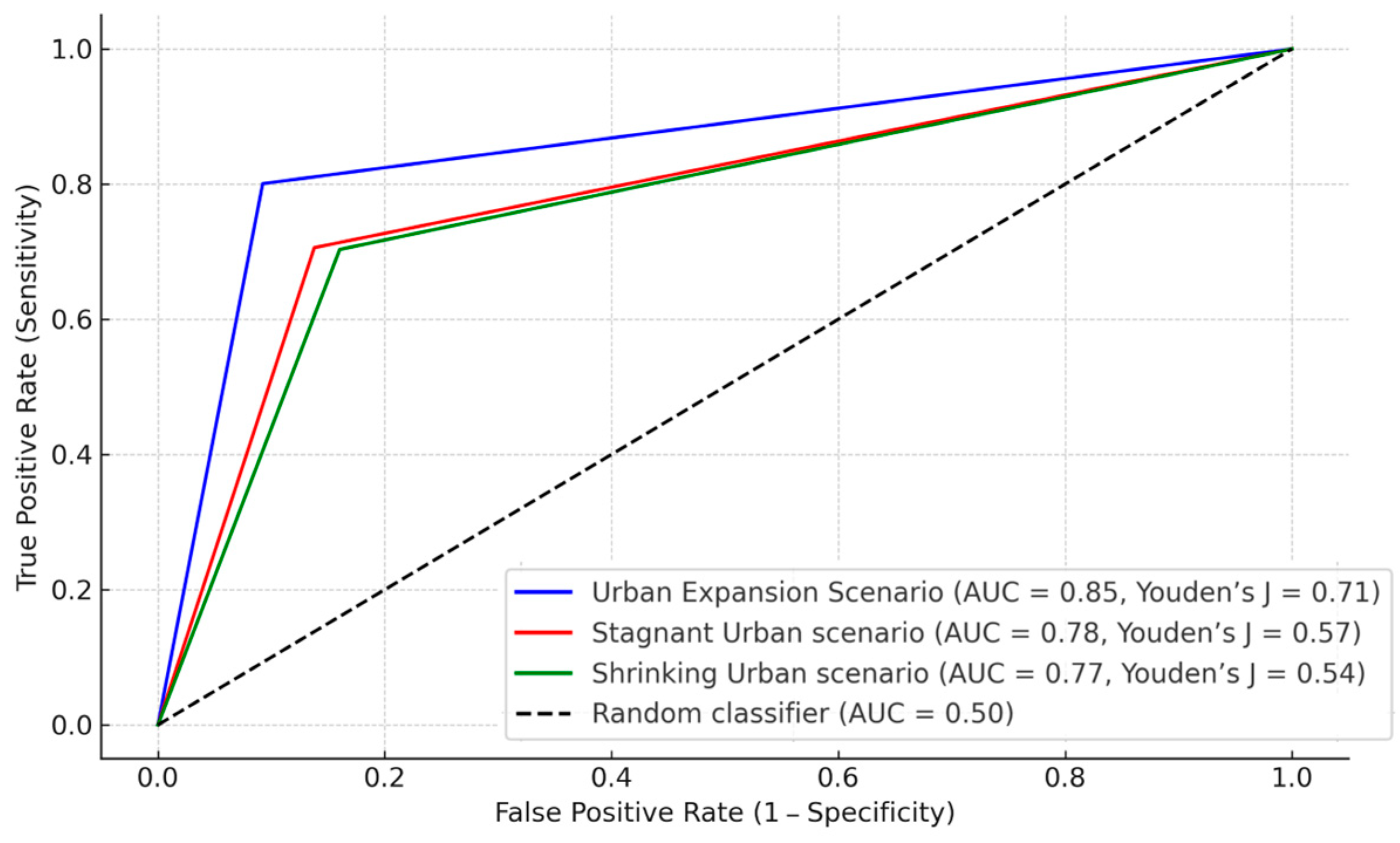
3.3. Model Validation and Accuracy
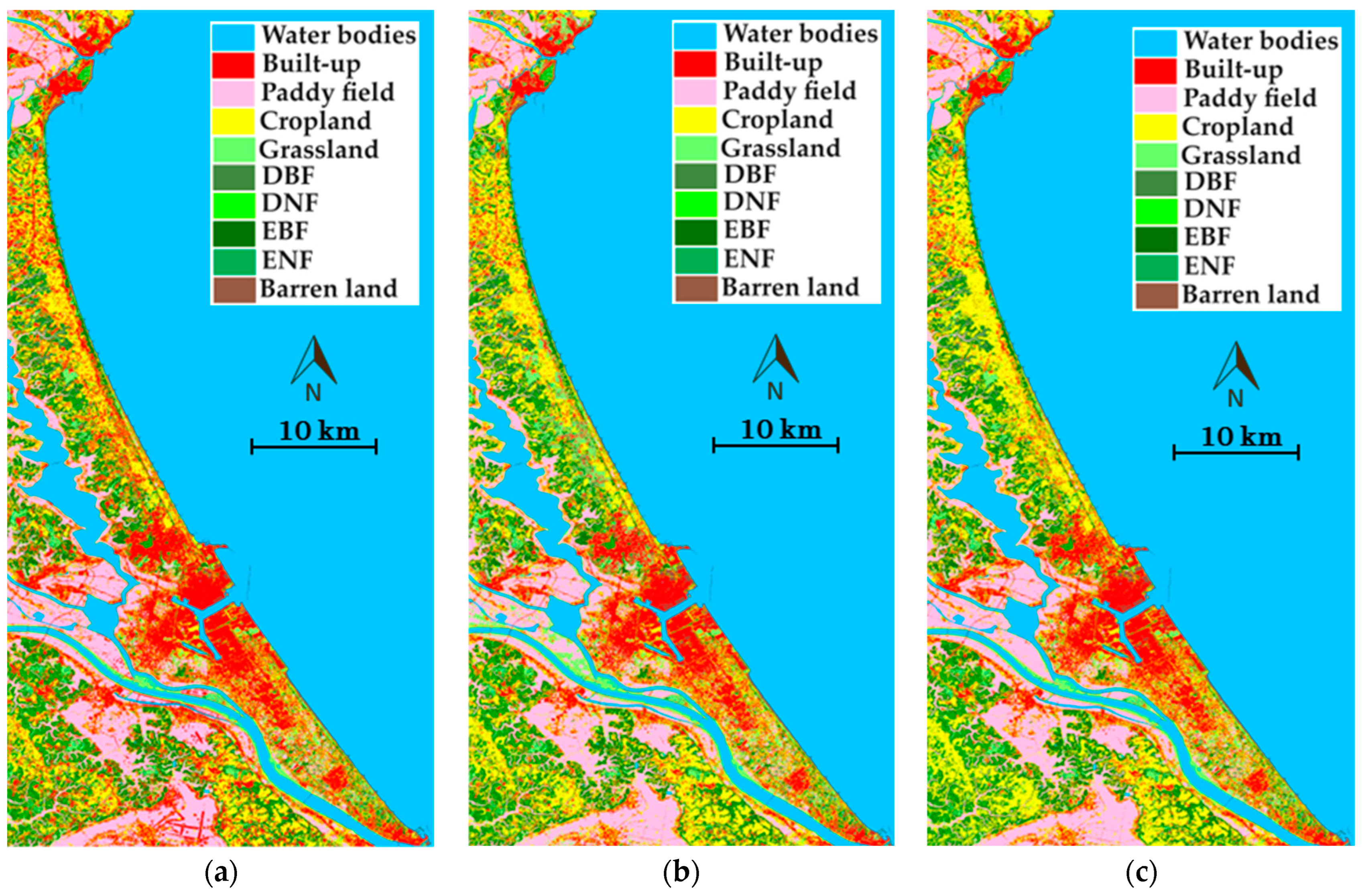
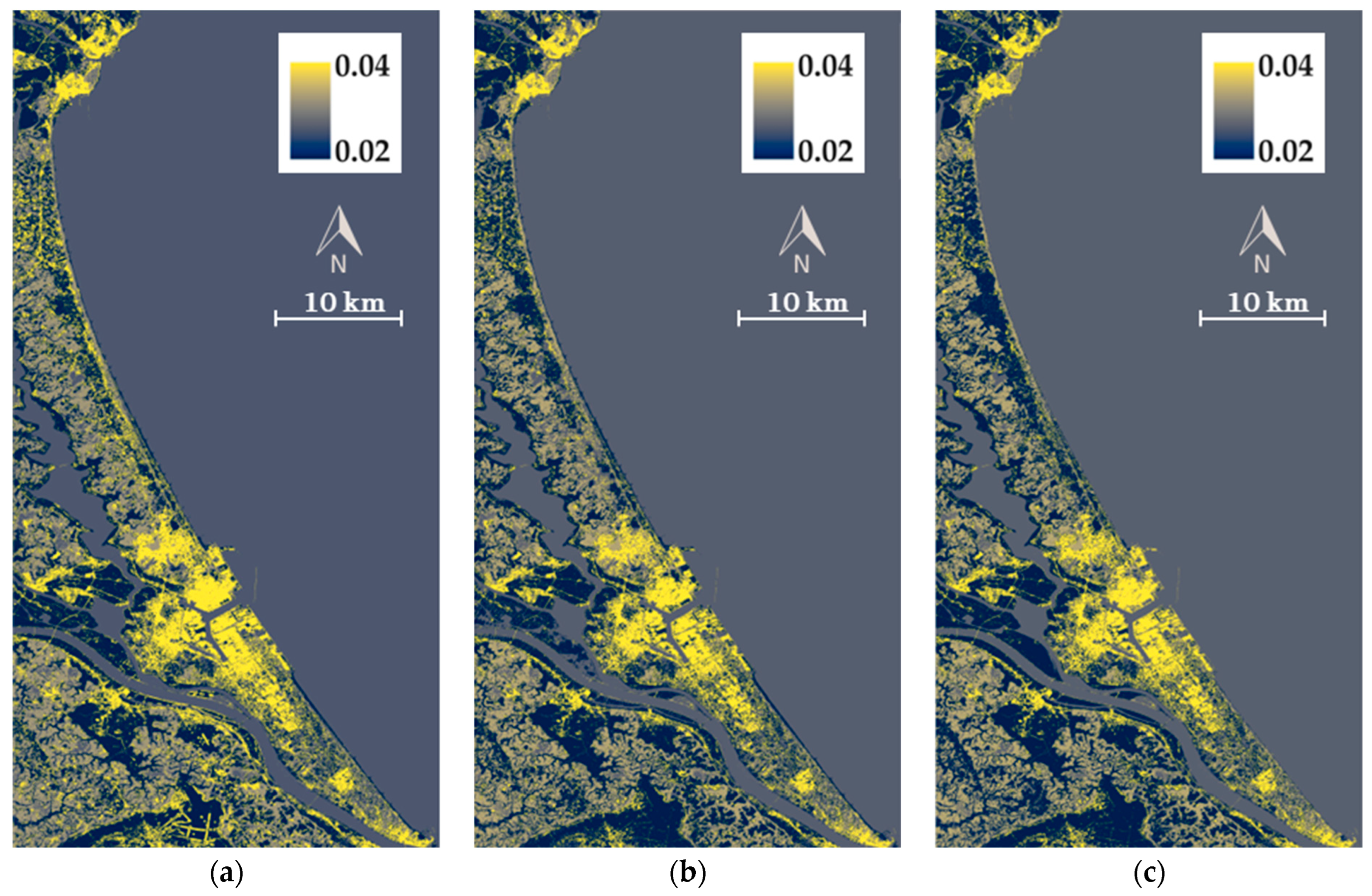
3.4. Modeling Future LULC Scenarios 2030 and Generating Roughness Maps Based on Predicted Outcomes
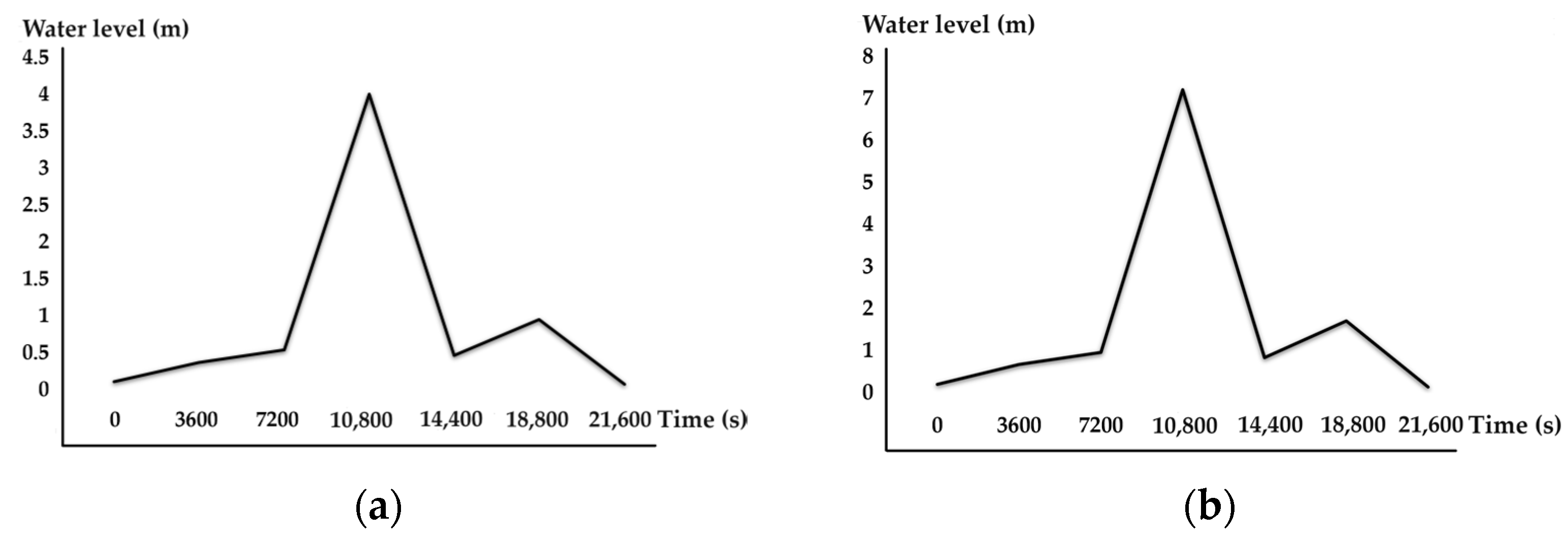
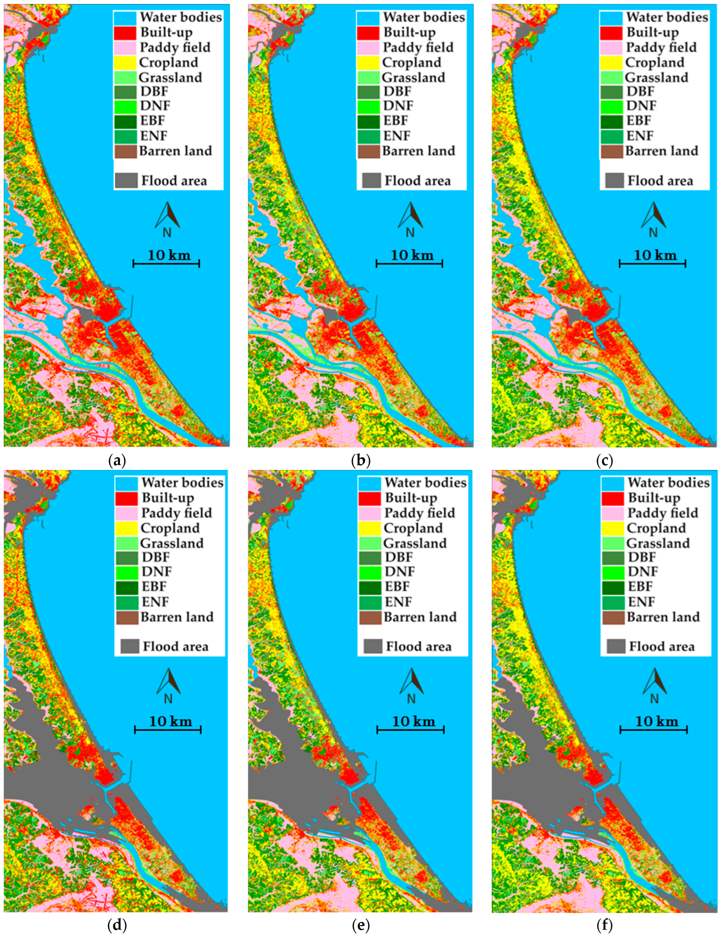
3.5. Flood Scenario Simulation with Input Water Levels
4. Discussion
4.1. Assessment and Associated Limitations of the Proposed Methodology
4.2. Review of LULC Modeling Outcomes
4.3. Flood Simulation Results
4.4. Future Work
5. Conclusions
Author Contributions
Funding
Institutional Review Board Statement
Informed Consent Statement
Data Availability Statement
Acknowledgments
Conflicts of Interest
References
- Wang, X.-J.; Tuo, Y.; Li, X.-F.; Feng, G.-L. Features of the new climate normal 1991–2020 and possible influences on climate monitoring and prediction in China. Adv. Clim. Chang. Res. 2023, 14, 930–940. [Google Scholar] [CrossRef]
- Syvitski, J.P.M.; Vörösmarty, C.J.; Kettner, A.J.; Green, P. Impact of humans on the flux of terrestrial sediment to the global coastal ocean. Science 2005, 308, 376–380. [Google Scholar] [CrossRef]
- Hinkel, J.; Lincke, D.; Vafeidis, A.T.; Perrette, M.; Nicholls, R.J.; Tol, R.S.J.; Marzeion, B.; Fettweis, X.; Ionescu, C.; Levermann, A. Coastal flood damage and adaptation costs under 21st century sea-level rise. Proc. Natl. Acad. Sci. USA 2014, 111, 3292–3297. [Google Scholar] [CrossRef] [PubMed]
- Syvitski, J.P.M.; Kettner, A.J.; Overeem, I.; Hutton, E.W.H.; Hannon, M.T.; Brakenridge, G.R.; Day, J.; Vörösmarty, C.; Saito, Y.; Giosan, L.; et al. Sinking deltas due to human activities. Nat. Geosci. 2009, 2, 681–686. [Google Scholar] [CrossRef]
- Tabari, H. Climate change impact on flood and extreme precipitation increases with water availability. Sci. Rep. 2020, 10, 13768. [Google Scholar] [CrossRef]
- Meehl, G.A.; Hu, A.; Tebaldi, C.; Arblaster, J.M.; Washington, W.M.; Teng, H.; Sanderson, B.M.; Ault, T.; Strand, W.G.; White, J.B., III. Relative outcomes of climate change mitigation related to global temperature versus sea-level rise. Nat. Clim. Chang. 2012, 2, 576–580. [Google Scholar] [CrossRef]
- de Graaf, R.; Hooimeijer, F. (Eds.) Urban Water in Japan; CRC Press: Boca Raton, FL, USA, 2008. [Google Scholar]
- Zhai, G.; Ikeda, S. Empirical analysis of Japanese flood risk acceptability within multi-risk context. Nat. Hazards Earth Syst. Sci. 2008, 8, 1049–1066. [Google Scholar] [CrossRef]
- Srinivasan, T.N.; Gopi Rethinaraj, T.S. Fukushima and thereafter: Reassessment of risks of nuclear power. Energy Policy 2013, 52, 726–736. [Google Scholar] [CrossRef]
- Suppasri, A.; Shuto, N.; Imamura, F.; Koshimura, S.; Mas, E.; Yalciner, A.C. Lessons learned from the 2011 great east japan tsunami: Performance of tsunami countermeasures, coastal buildings, and tsunami evacuation in japan. Pure Appl. Geophys. 2013, 170, 993–1018. [Google Scholar] [CrossRef]
- Carter, J.G.; Cavan, G.; Connelly, A.; Guy, S.; Handley, J.; Kazmierczak, A. Climate change and the city: Building capacity for urban adaptation. Prog. Plan. 2015, 95, 1–66. [Google Scholar] [CrossRef]
- Wu, X.; Wang, Z.; Guo, S.; Liao, W.; Zeng, Z.; Chen, X. Scenario-based projections of future urban inundation within a coupled hydrodynamic model framework: A case study in Dongguan City, China. J. Hydrol. 2017, 547, 428–442. [Google Scholar] [CrossRef]
- Reckien, D.; Salvia, M.; Heidrich, O.; Church, J.M.; Pietrapertosa, F.; De Gregorio-Hurtado, S.; D’Alonzo, V.; Foley, A.; Simoes, S.G.; Krkoška Lorencová, E.; et al. How are cities planning to respond to climate change? Assessment of local climate plans from 885 cities in the EU-28. J. Clean. Prod. 2018, 191, 207–219. [Google Scholar] [CrossRef]
- Lai, C.; Shao, Q.; Chen, X.; Wang, Z.; Zhou, X.; Yang, B.; Zhang, L. Flood risk zoning using a rule mining based on ant colony algorithm. J. Hydrol. 2016, 542, 268–280. [Google Scholar] [CrossRef]
- Zhao, L.; Liu, F. Land-use planning adaptation in response to SLR based on a vulnerability analysis. Ocean Coast. Manag. 2020, 196, 105297. [Google Scholar] [CrossRef]
- Canters, F.; Vanderhaegen, S.; Khan, A.Z.; Engelen, G.; Uljee, I. Land-use simulation as a supporting tool for flood risk assessment and coastal safety planning: The case of the Belgian coast. Ocean Coast. Manag. 2014, 101, 102–113. [Google Scholar] [CrossRef]
- Berry, M.; BenDor, T.K. Integrating sea level rise into development suitability analysis. Comput. Environ. Urban Syst. 2015, 51, 13–24. [Google Scholar] [CrossRef]
- Miller, M.M.; Shirzaei, M. Assessment of future flood hazards for southeastern Texas: Synthesizing subsidence, sea-level rise, and storm surge scenarios. Geophys. Res. Lett. 2021, 48, e2021GL092544. [Google Scholar] [CrossRef]
- Feng, Y.; Yang, Q.; Hong, Z.; Cui, L. Modelling coastal land use change by incorporating spatial autocorrelation into cellular automata models. Geocarto Int. 2018, 33, 470–488. [Google Scholar] [CrossRef]
- Lai, C.; Chen, X.; Wang, Z.; Yu, H.; Bai, X. Flood risk assessment and regionalization from past and future perspectives at basin scale. Risk Anal. 2020, 40, 1399–1417. [Google Scholar] [CrossRef] [PubMed]
- Moya, L.; Mas, E.; Koshimura, S. Learning from the 2018 western Japan heavy rains to detect floods during the 2019 Hagibis typhoon. Remote Sens. 2020, 12, 2244. [Google Scholar] [CrossRef]
- Liu, W.; Fujii, K.; Maruyama, Y.; Yamazaki, F. Inundation assessment of the 2019 Typhoon Hagibis in Japan using multi-temporal Sentinel-1 intensity images. Remote Sens. 2021, 13, 639. [Google Scholar] [CrossRef]
- Ohki, M.; Yamamoto, K.; Tadono, T.; Yoshimura, K. Automated processing for flood area detection using ALOS-2 and hydrodynamic simulation data. Remote Sens. 2020, 12, 2709. [Google Scholar] [CrossRef]
- Hattori, K.; Kaido, K.; Matsuyuki, M. The development of urban shrinkage discourse and policy response in Japan. Cities 2017, 69, 124–132. [Google Scholar] [CrossRef]
- Bloom, D.E.; Chatterji, S.; Kowal, P.; Lloyd-Sherlock, P.; McKee, M.; Rechel, B.; Rosenberg, L.; Smith, J.P. Macroeconomic implications of population ageing and selected policy responses. Lancet 2015, 385, 649–657. [Google Scholar] [CrossRef]
- Hartt, M.D. How cities shrink: Complex pathways to population decline. Cities 2018, 75, 38–49. [Google Scholar] [CrossRef]
- Ma, Z.; Zhou, G.; Zhang, J.; Liu, Y.; Zhang, P.; Li, C. Urban shrinkage in the regional multiscale context: Spatial divergence and interaction. Sustain. Cities Soc. 2024, 100, 105020. [Google Scholar] [CrossRef]
- Peng, W.; Wu, Z.; Duan, J.; Gao, W.; Wang, R.; Fan, Z.; Liu, N. Identifying and quantizing the non-linear correlates of city shrinkage in Japan. Cities 2023, 137, 104292. [Google Scholar] [CrossRef]
- Housing and Land Survey. Available online: https://www.stat.go.jp/english/data/jyutaku/index.html (accessed on 8 January 2024).
- Infrastructure Supporting Life and Economy, ‘Growing’ Ibaraki. Available online: https://www.pref.ibaraki.jp/soshiki/doboku/stock.html (accessed on 8 January 2024).
- Nguyen Hao, Q.; Takewaka, S. Shoreline changes along northern Ibaraki Coast after the Great East Japan Earthquake of 2011. Remote Sens. 2021, 13, 1399. [Google Scholar] [CrossRef]
- Coastal Conservation Master Plan. Available online: https://www.pref.ibaraki.jp/doboku/kasen/coast/032000.html (accessed on 8 January 2024).
- High-Resolution Land-Use and Land-Cover Map of Japan. Available online: https://www.eorc.jaxa.jp/ALOS/en/dataset/lulc/lulc_v2111_e.htm (accessed on 8 January 2024).
- GSI Maps. Available online: https://maps.gsi.go.jp/ (accessed on 8 January 2024).
- WorldPop Hub. Available online: https://hub.worldpop.org/ (accessed on 8 January 2024).
- Future Estimated Population Data by 500 m Mesh (H29 National Political Bureau Estimates). Available online: https://nlftp.mlit.go.jp/ksj/gml/datalist/KsjTmplt-mesh500.html (accessed on 8 January 2024).
- DioVISTA/Flood. Available online: https://www.hitachi-power-solutions.com/en/service/digital/diovista-flood/index.html (accessed on 8 January 2024).
- Shafizadeh-Moghadam, H.; Tayyebi, A.; Ahmadlou, M.; Delavar, M.R.; Hasanlou, M. Integration of genetic algorithm and multiple kernel support vector regression for modeling urban growth. Comput. Environ. Urban Syst. 2017, 65, 28–40. [Google Scholar] [CrossRef]
- Inouye, C.E.N.; de Sousa, W.C., Jr.; de Freitas, D.M.; Simões, E. Modelling the spatial dynamics of urban growth and land use changes in the north coast of São Paulo, Brazil. Ocean Coast. Manag. 2015, 108, 147–157. [Google Scholar] [CrossRef]
- Peng, W.; Fan, Z.; Duan, J.; Gao, W.; Wang, R.; Liu, N.; Li, Y.; Hua, S. Assessment of interactions between influencing factors on city shrinkage based on geographical detector: A case study in Kitakyushu, Japan. Cities 2022, 131, 103958. [Google Scholar] [CrossRef]
- Bernt, M. The limits of shrinkage: Conceptual pitfalls and alternatives in the discussion of urban population loss: Debates & developments. Int. J. Urban Reg. Res. 2016, 40, 441–450. [Google Scholar]
- Döringer, S.; Uchiyama, Y.; Penker, M.; Kohsaka, R. A meta-analysis of shrinking cities in Europe and Japan. Towards an integrative research agenda. Eur. Plan. Stud. 2020, 28, 1693–1712. [Google Scholar] [CrossRef]
- Hori, K.; Saito, O.; Hashimoto, S.; Matsui, T.; Akter, R.; Takeuchi, K. Projecting population distribution under depopulation conditions in Japan: Scenario analysis for future socio-ecological systems. Sustain. Sci. 2021, 16, 295–311. [Google Scholar] [CrossRef]
- Kubo, T.; Yui, Y. The Rise in Vacant Housing in Post-Growth Japan; Springer: Singapore, 2019; 175p. [Google Scholar]
- Zhang, Y.; Fu, Y.; Kong, X.; Zhang, F. Prefecture-level city shrinkage on the regional dimension in China: Spatiotemporal change and internal relations. Sustain. Cities Soc. 2019, 47, 101490. [Google Scholar] [CrossRef]
- Sarkar, D.; Saha, S.; Mondal, P. GIS-based frequency ratio and Shannon’s entropy techniques for flood vulnerability assessment in Patna district, Central Bihar, India. Int. J. Environ. Sci. Technol. 2022, 19, 8911–8932. [Google Scholar] [CrossRef]
- Htet, H.; Khaing, S.S.; Myint, Y.Y. Tweets sentiment analysis for healthcare on big data processing and IoT architecture using maximum entropy classifier. In Advances in Intelligent Systems and Computing; Springer: Singapore, 2019; pp. 28–38. [Google Scholar]
- Safabakhshpachehkenari, M.; Tonooka, H. Assessing and enhancing predictive efficacy of machine learning models in urban land dynamics: A comparative study using multi-resolution satellite data. Remote Sens. 2023, 15, 4495. [Google Scholar] [CrossRef]
- Haghighat, F. Predicting the trend of indicators related to COVID-19 using the combined MLP-MC model. Chaos Solitons Fractals 2021, 152, 111399. [Google Scholar] [CrossRef]
- Mansour, S.; Ghoneim, E.; El-Kersh, A.; Said, S.; Abdelnaby, S. Spatiotemporal monitoring of urban sprawl in a coastal city using GIS-based Markov Chain and artificial Neural Network (ANN). Remote Sens. 2023, 15, 601. [Google Scholar] [CrossRef]
- Saeidi, S.; Mohammadzadeh, M.; Salmanmahiny, A.; Mirkarimi, S.H. Performance evaluation of multiple methods for landscape aesthetic suitability mapping: A comparative study between Multi-Criteria Evaluation, Logistic Regression and Multi-Layer Perceptron neural network. Land Use Policy 2017, 67, 1–12. [Google Scholar] [CrossRef]
- Bratley, K.; Ghoneim, E. Modeling urban encroachment on the agricultural land of the Eastern Nile Delta using remote sensing and a GIS-based Markov Chain model. Land 2018, 7, 114. [Google Scholar] [CrossRef]
- Lin, W.; Sun, Y.; Nijhuis, S.; Wang, Z. Scenario-based flood risk assessment for urbanizing deltas using future land-use simulation (FLUS): Guangzhou Metropolitan Area as a case study. Sci. Total Environ. 2020, 739, 139899. [Google Scholar] [CrossRef]
- Smirnova, D.A.; Medvedev, I.P. Extreme Sea Level Variations in the Sea of Japan Caused by the Passage of Typhoons Maysak and Haishen in September 2020. Russ. Acad. Sci. Oceanol. 2023, 63, 623–636. [Google Scholar] [CrossRef]
- Yamaguchi, S.; Ikeda, T.; Iwamura, K. Rapid flood simulation software for personal computer with Dynamic Domain Defining Method. In Proceedings of the 4th International Symposium on Flood Defence: Managing Flood Risk, Reliability and Vulnerability, Toronto, ON, Canada, 6–8 May 2008. [Google Scholar]
- Connell, R.J.; Painter, D.J.; Beffa, C. Two-dimensional flood plain flow. II: Model validation. J. Hydrol. Eng. 2001, 6, 406–415. [Google Scholar] [CrossRef]
- Yamaguchi, S.; Ikeda, T.; Yamaho, S. Flood risk assessment system for major metropolitan areas in Japan. In Proceedings of the 10th International Conference on Hydroinformatics (HIC 2012), Hamburg, Germany, 14–18 July 2012. [Google Scholar]
- Yamaguchi, S.; Ikeda, T. Automatic integration of hydraulic and hydrologic models based on geographic information. In Proceedings of the 9th International Conference on Hydroinformatics (HIC 2010), Tianjin, China, 7–11 September 2010. [Google Scholar]
- Xia, Y. Chapter Eleven—Correlation and association analyses in microbiome study integrating multiomics in health and disease. Prog. Mol. Biol. Transl. Sci. 2020, 171, 309–491. [Google Scholar]
- Mogaraju, J.K. Artificial Intelligence assisted prediction of land surface temperature (LST) based on significant air pollutants over the Annamayya district of India. Res. Sq. 2023. [Google Scholar] [CrossRef]
- Available online: https://www.mlit.go.jp/river/shishin_guideline/kaigan/takashioshinsui_manual.pd (accessed on 30 April 2023).
- Ouyang, M.; Kotsuki, S.; Ito, Y.; Tokunaga, T. Employment of hydraulic model and social media data for flood hazard assessment in an urban city. J. Hydrol. Reg. Stud. 2022, 44, 101261. [Google Scholar] [CrossRef]
- Tursina, S.; Kato, S.; Afifuddin, M. Incorporating dynamics of land use and land cover changes into tsunami numerical modelling for future tsunamis in Banda Aceh. E3S Web Conf. 2022, 340, 01014. [Google Scholar] [CrossRef]


| Simulation Scenario | Explanatory Variables | Accuracy Rate | Skill Measure | Influence Order |
|---|---|---|---|---|
| 1- Urban Expansion | 1- Proximity to the urban center | 60.95 | 0.5313 | 4 |
| 2- Proximity to dense population | 60.80 | 0.5296 | 7 | |
| 3- DEM | 46.61 | 0.3593 | 2 | |
| 4- Probability distribution of transition to urban | 50.49 | 0.4059 | 3 | |
| 5- Urban spatial trends | 55.68 | 0.4682 | 10 | |
| 6- Nlog transformation of urban distance | 34.87 | 0.2184 | 1 | |
| 7- PCR (2020–2025) | 57.59 | 0.4911 | 5 | |
| 8- Slope | 60.92 | 0.5310 | 8 | |
| 9- Proximity to the road | 60.93 | 0.5312 | 9 | |
| 10- Road map | 60.72 | 0.5286 | 6 | |
| 2- Urban Stability and Grassland Expansion | 1- Proximity to dense population | 45.75 | 0.2767 | 4 |
| 2- Population distribution | 45.55 | 0.2740 | 3 | |
| 3- Population distribution age 65+ | 43.48 | 0.2464 | 2 | |
| 4- Probability distribution of transition to grassland | 35.14 | 0.1352 | 1 | |
| 5- PCR (2011–2020) | 45.81 | 0.2775 | 7 | |
| 6- PCR (2020–2030) | 46.31 | 0.2841 | 11 | |
| 7- Proximity to dense population of 2025 | 45.82 | 0.2776 | 10 | |
| 8- DEM | 45.80 | 0.2773 | 6 | |
| 9- Slope | 45.81 | 0.2775 | 8 | |
| 10- Proximity to the urban center | 45.82 | 0.2775 | 9 | |
| 11- Grassland spatial trends | 45.78 | 0.2571 | 5 | |
| 3- Urban Shrinkage | 1- Proximity to dense population | 53.94 | 0.3091 | 6 |
| 2- Population distribution | 54.77 | 0.3215 | 9 | |
| 3- Population distribution age 65+ | 44.57 | 0.1686 | 1 | |
| 4- Probability distribution of shrinkage | 51.03 | 0.2654 | 4 | |
| 5- PCR (2011–2020) | 53.85 | 0.3077 | 5 | |
| 6- PCR (2020–2030) | 49.54 | 0.2431 | 3 | |
| 7- Proximity to dense population of 2025 | 54.01 | 0.3102 | 7 | |
| 8- DEM | 46.54 | 0.1980 | 2 | |
| 9- Slope | 54.78 | 0.3218 | 10 | |
| 10- Proximity to dense population of 2030 | 54.88 | 0.3231 | 11 | |
| 11- Shrinking spatial trends | 54.34 | 0.3152 | 8 |
| Indicators | Simulation Scenario | ||
|---|---|---|---|
| 1- Urban Expansion | 2- Urban Stability and Grassland Expansion | 3- Urban Shrinkage | |
| Kappa | 88.66 | 85.33 | 88.22 |
| F1 score | 0.8568 | 0.7912 | 0.7817 |
| MCC | 0.7001 | 0.5461 | 0.5255 |
Disclaimer/Publisher’s Note: The statements, opinions and data contained in all publications are solely those of the individual author(s) and contributor(s) and not of MDPI and/or the editor(s). MDPI and/or the editor(s) disclaim responsibility for any injury to people or property resulting from any ideas, methods, instructions or products referred to in the content. |
© 2024 by the authors. Licensee MDPI, Basel, Switzerland. This article is an open access article distributed under the terms and conditions of the Creative Commons Attribution (CC BY) license (https://creativecommons.org/licenses/by/4.0/).
Share and Cite
Safabakhshpachehkenari, M.; Tonooka, H. Modeling Land Use Transformations and Flood Hazard on Ibaraki’s Coastal in 2030: A Scenario-Based Approach Amid Population Fluctuations. Remote Sens. 2024, 16, 898. https://doi.org/10.3390/rs16050898
Safabakhshpachehkenari M, Tonooka H. Modeling Land Use Transformations and Flood Hazard on Ibaraki’s Coastal in 2030: A Scenario-Based Approach Amid Population Fluctuations. Remote Sensing. 2024; 16(5):898. https://doi.org/10.3390/rs16050898
Chicago/Turabian StyleSafabakhshpachehkenari, Mohammadreza, and Hideyuki Tonooka. 2024. "Modeling Land Use Transformations and Flood Hazard on Ibaraki’s Coastal in 2030: A Scenario-Based Approach Amid Population Fluctuations" Remote Sensing 16, no. 5: 898. https://doi.org/10.3390/rs16050898