Article

Tracking the 2D/3D Morphological Changes of Tidal Flats Using Time Series Remote Sensing Data in Northern China

1
Key Laboratory of Spatial Data Mining and Information Sharing of Ministry of Education, National & Local Joint Engineering Research Center of Satellite Geospatial Information Technology, Fuzhou University, Fuzhou 350108, China
2
State Key Laboratory of Estuarine and Coastal Research, East China Normal University, Shanghai 200050, China
3
Lancaster Environment Centre, Lancaster University, Lancaster LA1 4YQ, UK
*
Author to whom correspondence should be addressed.
Remote Sens. 2024, 16(5), 886; https://doi.org/10.3390/rs16050886
Submission received: 15 January 2024 / Revised: 21 February 2024 / Accepted: 29 February 2024 / Published: 2 March 2024
(This article belongs to the Special Issue Remote Sensing for Geology and Mapping)

Abstract

:
Tidal flats in northern China are essential parts of the East Asian-Australasian Flyway, the densest pathway for migratory waterbirds, and are of great ecological and economic importance. They are threatened by human activities and climate change, raising the urgency surrounding tracking the spatiotemporal dynamics of tidal flats. However, there is no cost-effective way to map morphological changes on a large spatial scale due to the inaccessibility of the mudflats. In this study, we proposed a pixel-based multi-indices tidal flat mapping algorithm that precisely characterizes 2D/3D morphological changes in tidal flats in northern China using time-series remote sensing data. An overall accuracy of 0.95 in delineating tidal flats to a 2D extent was achieved, with 11,716 verification points. Our results demonstrate that the reduction in sediment discharge from rivers along the coastlines of the Yellow and Bohai Seas has resulted in an overall decline in the area of tidal flats, from 4856.40 km2 to 4778.32 km2. Specifically, 3D analysis showed that significant losses were observed in the mid-to-high-tidal flat zones, while low-elevation tidal flats experienced an increase in area due to the transformations in mid-to-high-tidal flats. Our results indicate that the sediment inputs from rivers and the succession of native vegetation are the primary drivers leading to 2D/3D morphological changes of tidal flats following the cessation of extensive land reclamation in northern China.

1. Introduction

Tidal flats, situated between the average high tide and average low tide lines, are integral components of coastal zones [1]. They act as transitional zones linking terrestrial and marine ecosystems [2] and provide a number of ecological services, including storm surge protection and carbon sequestration [3,4]. Tidal flats also provide habitats for a diverse range of wildlife, including migratory birds [5], fish, and other marine organisms [6,7]. Moreover, they play a crucial role in supporting economic activities such as port facilities, tourism, and fisheries [3,8]. Global tidal flats have decreased in area by 16% (>20,000 km2) [9]. Approximately 10% of the global population resides in coastal regions with elevations below 10 m [10]. However, tidal flats face increasing threats from human activities, such as land reclamation [11,12] and aquaculture [13], which amplifies the exposure of tidal flats to coastal erosion [14] and rising sea levels driven by climate change [15,16]. It is crucial to carefully consider the balance between the preservation and utilization of tidal flats to ensure the future sustainable development of coastal areas. Therefore, accurate monitoring and understanding of the spatial distribution and temporal changes in tidal flat morphology are of paramount importance and necessity.
The tidal flats in northern China, along with the shorelines of the Yellow Sea and Bohai Sea (YBS), have exhibited tremendous losses in tidal flat area due to extensive land reclamation over the past decades. These wetlands constitute a core component of the East Asian-Australasian Flyway, one of the densest pathways for migratory waterbirds. The area of tidal flats in the YBS has been drastically reduced by 39.2% from 1981 to 2016 due to human activities [17]. The Chinese government has implemented stringent bans on marine utilization since 2018 in an attempt to cease the continuous loss of tidal flats over the past decades. However, the fate of tidal flats in the YBS is still ambiguous as they are exposed to risks in the form of sediment starvation and sea level rise [18,19]. Therefore, large-scale mapping with timely updates is needed to track the 2D/3D morphological changes of tidal flats in the YBS after the bans.
Poor accessibility and highly dynamic challenges pose great obstacles to the morphological mapping of tidal flats [20], resulting in a morphological data gap in these areas. Various techniques have been employed to reconstruct the morphology of tidal flats. Conventional in situ measurement methods, such as use of the Real-Time Kinematic Global Navigation Satellite System and the total station [21], are time-consuming and labor intensive and can only collect limited data in a small region with sparse samples. The rise of unmanned aerial vehicles (UAV) [22] and airborne LiDAR [23] has enabled the acquisition of precise digital elevation models with high spatial resolution for localized, small patches of observed areas. Nevertheless, the high cost of UAV and airborne LiDAR limits timely updates of morphological data in space and time. Since the first launch of the Earth observation satellite in the 1970s, remote sensing (RS) has provided the potential for rapid monitoring of the surface of Earth on a large spatiotemporal scale. Using remote sensing data to map morphological changes in tidal flats, with large spatial coverage and frequent updates, has emerged as a widely adopted and cost-effective approach.
The waterline method [24] is a commonly employed approach to derive tidal flats morphology using satellite images and has been applied in various regions worldwide [25,26,27,28]. It entails extracting waterlines from time remote sensing images and assigning measured or simulated tidal elevation information to these waterlines, then reconstructing the three-dimensional morphology of tidal flats by interpolating the assigned tidal values. However, there are uncertainties in morphological data on a large scale derived from the waterline method due to the spatial inconsistency in the elevation of waterlines [29]. Recently, a pixel-based morphology mapping method was adopted to reconstruct the three-dimensional morphology of tidal flats [30,31], which links the inundation frequency to the tidal flat elevation of pixels to mitigate the spatial inconsistency of waterline height on a large scale. This method is easy to reproduce in other regions since it relies only on a simple remote sensing index [31,32]. The key to reconstructing high-precision morphology of tidal flats is to classify the water and land area accurately in each image. However, in the context of large-scale tidal flats morphology mapping, variations in sediment input from rivers lead to substantial disparities in the concentration of suspended sediment in coastal waters, which introduces great uncertainty to morphological mapping. Therefore, water-land separation should employ different water indices based on coastal water bodies. Thus, two primary research questions needed to be well addressed in our study:
(1)
How can we accurately extract the water surface area, at different degrees of turbidity, of coastal water over a large spatial scale?
(2)
How do tidal flats change in 2D/3D scale after the cessation of coastal reclamation, and what are the main drivers?
To address the aforementioned issues, this study aims to develop a pixel-based, multi-indices tidal flats mapping algorithm (PMITMA) to accurately delineate 2D/3D morphological changes in tidal flats using multiple sources of time-series remote sensing imagery on the Google Earth Engine (GEE) platform. Based on the application of tidal flats in the YBS, we will have a better understanding of spatiotemporal and morphological changes in tidal flats in the YBS after institution of the marine utilization bans and the influence of continuous human activities.

2. Material and Methods
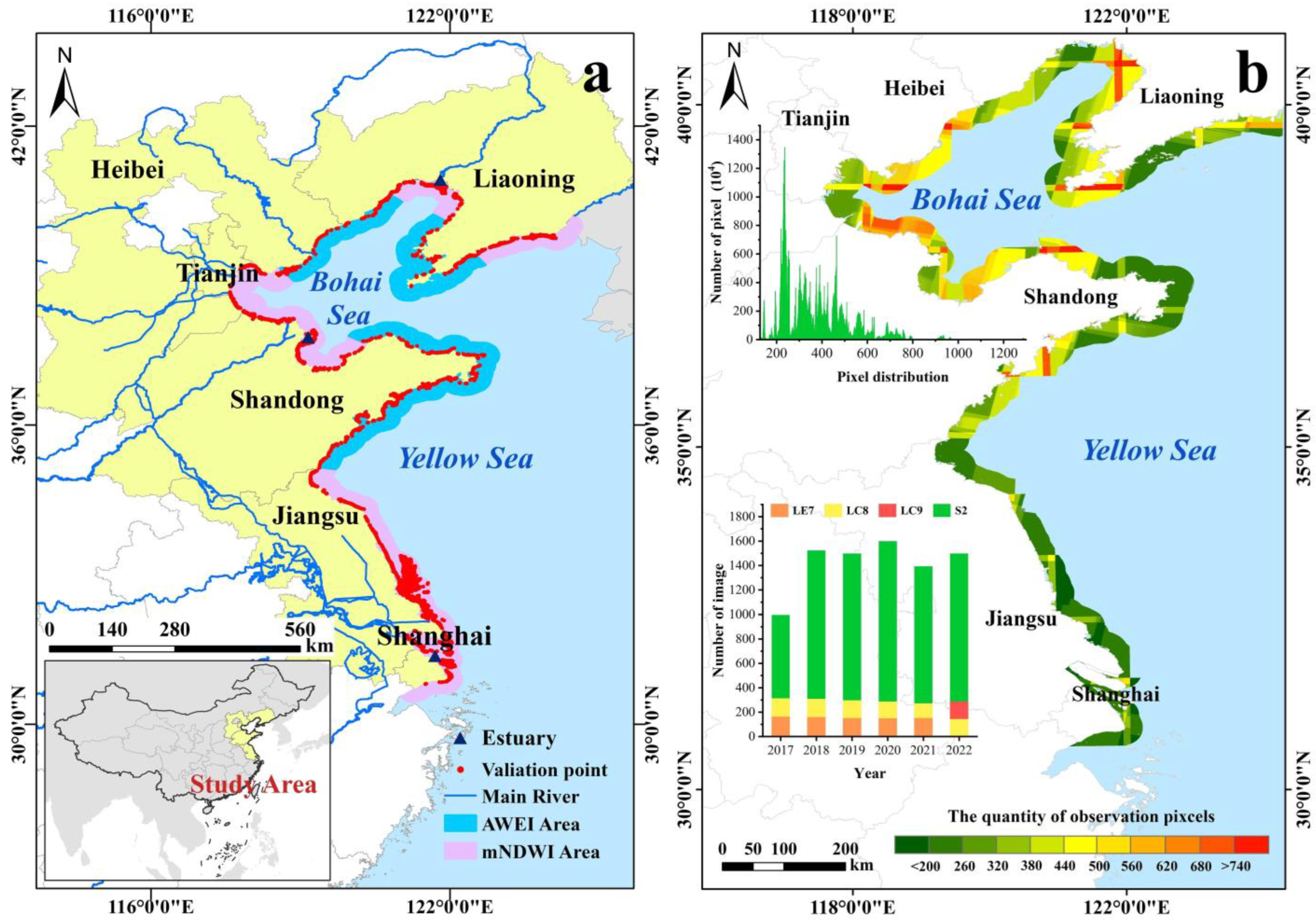
2.1. Study Area

The study region extends from the Yalu River Estuary to the Yangtze River Delta region in China (30°38′–41°03′N, 117°29′–122°03′E) (Figure 1a). The region north of 34°20′N is characterized by a temperate monsoon climate, whereas the southern portion has a subtropical monsoon climate. The mean annual temperature ranges from 5 to 20 °C, and the average annual precipitation varies from 400 to 1300 mm [33]. The coastline stretches approximately 7978 km and passes through the provincial districts of Liaoning, Hebei, Tianjin, Shandong, Jiangsu, and Shanghai, with around 60 million people inhabiting the low-lying coastal regions. The staggering population pressure is driving the rapid expansion of cities, industries, and agriculture, which in turn encroaches upon the already limited space of tidal flats [34].
In the past half-century, sediment in the Yellow and Bohai Seas has primarily originated from three major rivers, namely the Yellow River, Yangtze River, and Liao River [35], including underwater sand from the abandoned mouth of the Yellow River [36]. During the Ming and Qing dynasties, the Yellow River discharged a significant amount of sediment into the Yellow Sea through the Huai River, contributing to sedimentation in northern Jiangsu. However, the diversion of the Yellow River into the Bohai Sea in 1855 led to the gradual abandonment of the Yellow River Delta in northern Jiangsu, resulting in the formation of extensive underwater sandbars. Over the past 22 years, the annual average sediment input from the Yellow River and Yangtze River has significantly decreased by 292 million and 371 million tons, respectively, representing a reduction of 81.33% and 60.80% compared to the previous decades of the last century. The average concentration of suspended sediment in the nearshore waters of these areas ranges from approximately 40–80 mg/L, while ranging from 20–40 mg/L along the coast on either side of the river mouths [37]. These sediments, nurtured by the combined forces of ocean currents, have contributed to the formation of significant tidal flat wetlands, including the Yellow River Delta, Yangtze River Delta, and Liao River Delta, as well as radiating sandbars in central Jiangsu. These tidal flat wetlands provide ecosystem services worth approximately $30 billion annually [34]. The width of the major tidal flats can reach up to 25 km in the Bohai and Yellow Seas. Therefore, the study area is delimited to within a 25 km buffer of the coastline.

2.2. Data Sources

In this study, we utilized two widely used and freely accessible satellite datasets, the Landsat series and Sentinel-2A/B. The Landsat 7/8/9 satellites cover a broad range of wavelengths, spanning from visible to thermal infrared, making them suitable for identifying coastal water bodies. The bands of Landsat series images have a spatial resolution of 30 m, and the satellites revisit the same area every 16 days. The Sentinel-2, equipped with the Multi-Spectral Imager (MSI), encompasses similar spectral bands as the Landsat series. Furthermore, the Sentinel-2 satellites offer a higher spatial resolution. The blue, green, red, and near-infrared band channels have a resolution of 10 m. Moreover, the Sentinel-2 satellites revisit the same area every 5 days.
The integrated utilization of these two satellites enables more frequent observations of the tidal flats, enhancing the temporal resolution of remote sensing imagery and providing detailed and accurate information for monitoring surface changes and environmental dynamics. We utilized a total of 1776 images from the Landsat7/8/9 satellite and 6272 images from the Sentinel-2 spanning from 1 January 2017 to 31 December 2022 (Figure 1b). These image data are divided into three periods, including 2017–2018, 2019–2020, and 2021–2022, in order to conduct the time-series analysis for tidal flats mapping of time stages in the YBS. To mitigate the influence of cloud coverage on earth observation, we selected images with a cloud cover of less than 30% and utilized the bitmask band from Sentinel-2 images and Landsat images to mask the pixels covered by opaque and cirrus clouds. Figure 1b illustrates the distribution of observation pixels across the entire study area after masking.

2.3. Pixel-Based Multi-Indices Tidal Flat Mapping Algorithm

A pixel-based multi-indices tidal flat mapping algorithm was developed to accurately map the morphology of tidal flats in the YBS using the GEE platform. It encompasses three key components: (1) water frequency generation from time-series images, (2) tidal flats extraction, and (3) accuracy assessment (Figure 2).

2.3.1. Assessing Temporal Changes in Coastline

The extensive and meandering coastline of the Yellow and Bohai Seas exhibits varying suspended sediment content in its nearshore water bodies [37,38]. Various water indices exhibit different levels of effectiveness in differentiating between tidal flats and water bodies. Hence, the selection of a suitable water index should be based on the sediment content of these bodies. The most commonly used water indices [39] for water-land separation are the Normalized Difference Water Index (NDWI) [40], the modified Normalized Difference Water Index (mNDWI) [41], and the Automated Water Extraction Index (AWEI) [42] (Table 1). NDWI, the initially proposed water index, calculates the reflectance of green and near-infrared bands to effectively differentiate between clear water bodies and land. The mNDWI, an enhanced variant of NDWI that utilizes the shortwave infrared band instead of the near-infrared band, improves its sensitivity [43] and more accurately extracts water bodies. AWEI was originally developed to mask water bodies influenced by shadows cast by clouds, buildings, and mountains, and it consistently exhibits excellent performance across diverse water types and quality conditions [44,45,46,47]. To compare the dynamic characteristics of different water indices on tidal flats and water bodies, we selected 24 images (one image per month) from the high turbid regions of the Yellow River Estuary and the Yangtze River Estuary, captured in 2021. A total of 1440 sample points were collected by selecting 30 sample points each from water bodies and tidal flats along the water-land boundary in every image. The values of three water indices for the sample points were obtained. According to the results (Figure 3), NDWI did not effectively separate water bodies (Figure 3(a1,b1)) from tidal flats in January, March, August, September, and November. In contrast, AWEI (Figure 3(a3,b3)) successfully separated water bodies in all months except January, while mNDWI (Figure 3(a2,b2)) demonstrated the highest degree of separation among all the indices. Consistent with previous research findings, mNDWI is often suitable for areas with relatively turbid water, but it may lead to over-extraction in some clear water areas [48]. Accordingly, a few points in the figure showing tidal flats were misclassified as water bodies by mNDWI. AWEI demonstrated higher accuracy than NDWI in extracting clear water bodies [49,50] and also exhibited better extraction capabilities in slightly turbid water areas (Figure 3). Based on thorough consideration, we have determined that mNDWI will be applied in the Yalu River Basin, Liaohe Basin, Yellow River Basin, and Yangtze River Basin, whereas AWEI will be employed in the remaining regions (Figure 1a).

2.3.2. Water Frequency Generation from Time Series Images

Some studies directly employ threshold segmentation for water-land separation. This is a simple pixel-level comparison method. However, for large-scale image data and large-scale regions, there are significant differences in grayscale values between different images and areas. It can be challenging to determine a universal threshold that can adapt to the classification requirements of the most complex regions [51,52], especially in turbid water areas. Thus, a semi-automated method integrated with the K-Means++ algorithm [53], which is an unsupervised classifier, along with georeferenced points, was used to separate water and land pixels in the time series water index images (Figure 4). Herein, the utilization of the K-means++ initialization method enhanced the clustering results by ensuring a more even distribution of the initial centroids, decreasing the likelihood of suboptimal solutions that can arise from random initialization in the traditional K-means algorithm. Through our multiple experiments (set cluster numbers ranging from two to 10) with visual comparison, we found that the K-mean++ algorithm achieves optimal performance for land-water separation when the number of clusters is set to six (Figure 4c). By incorporating additional georeferenced points (Figure 4c), the points intersecting with the six clusters were classified as water, while the rest were classified as land (Figure 4d). Thus, the binary image of land and water area was generated from every single image of the time-series (Figure 4d). The water frequency is calculated on a pixel-by-pixel basis using the binary time-series images over each study period (Figure 4e). The calculation formula is as follows:
f x , y = i = 1 n B k x , y n
where x , y represents the spatial coordinates of each pixel, f x , y is the water frequency of each pixel, n is the number of binary images, and B k x , y is the binary image of the k-th scene.

2.3.3. Tidal Flat Extraction

Tidal flats can be more effectively identified in a water frequency map. We adopted thresholds of 0.05 and 0.95 to determine the upper and lower boundaries of tidal wetlands, as it has been empirically proven effective [54]. It is worth noting that the presence of vegetation on tidal flats significantly influences the accuracy of tidal flats terrain mapping, as their height exceeds that of the tidal flats. Therefore, we adopted the Maximum Spectral Index Composite (MSIC) method to generate an NDVI-MSIC map to determine the largest potential area of vegetation presence. Subsequently, the K-means++ method described in the previous section was applied to construct a binary vegetation map for masking vegetation.
Nonetheless, certain features present in both land and sea, such as reservoirs, fish farms, fish rafts, scattered clouds, and other objects with high fluctuation, can affect the accurate extraction of tidal flats. Consequently, to address this issue, an artificial coastline was employed to mask inland areas, and the “connectedPixelCount” function in GEE was utilized to remove pixel clusters containing fewer than 120 units. A negative correlation exists between the elevation of the intertidal zone and the frequency of tidal inundation [30]. Tidal flats with higher elevations exhibit a low frequency of water submergence, approaching zero, whereas tidal flats with lower elevations experience a high frequency of water submergence, approaching one. Therefore, we calculated the one-water frequency for each grid of the obtained water frequency map in ArcGIS to represent the relative elevation frequency of tidal flats (Figure 4f). The relative elevation values range from 0.05 to 0.95, with 0.95 representing the highest point and 0.05 representing the lowest point of the tidal flats.

2.3.4. Accuracy Assessment

To validate the accuracy of the tidal flats map, two methods were employed to assess the accuracy. A total of 21,171 validation points were collected from the lowest-tide images (Figure 1a) from Sentinel-2 from 2017 to 2022 and high-resolution imagery from Google Earth and used for the accuracy assessment of RS-derived tidal flats. Strategic selection of tidal gauge stations situated along the nearshore areas of the Yellow and Bohai Seas was performed, and 23 in total were chosen in order to guarantee at least one tidal gauge station in each path/row of the satellite images. These points were categorized into tidal flats and non-tidal flats, e.g., water, vegetation, and land. The seaward edge detection of tidal flats is key to verifying the accuracy of RS-derived tidal flats products, and 11,716 validation points were located at the seaward edges of the tidal flats (Figure 1a). A confusion matrix and the F1 score were employed to evaluate the accuracy of tidal flats with the following equation:
F 1 S c o r e = 2 T P 2 T P + F N + F P
where TP represents the count of correctly classified tidal flats samples, FP represents the count of incorrectly classified non-tidal flat samples as tidal flats, and FN represents the count of incorrectly classified tidal flats samples as non-tidal flats. Secondly, we compared the results by overlaying the lowest tide images. The aforementioned experiments were conducted on GEE.

3. Results

3.1. Accuracy Assessment Result

The accuracy of coastal land cover maps was assessed for three periods (Table 2). Results showed that the year 2020 achieved the highest accuracy with an overall precision of 95.83%. The validation results indicate that the tidal flat extent delineated by PMTMA aligns closely with the validation sites. Detailed accuracy evaluation results for each period are provided in Table 2.
We tested the relative elevation with ICESat-2 derived elevation of tidal flats, revealing a p-value of less than 0.01 and R2 (Figure 5), indicating a significant positive correlation between relative elevation and ICESat-2 elevation.

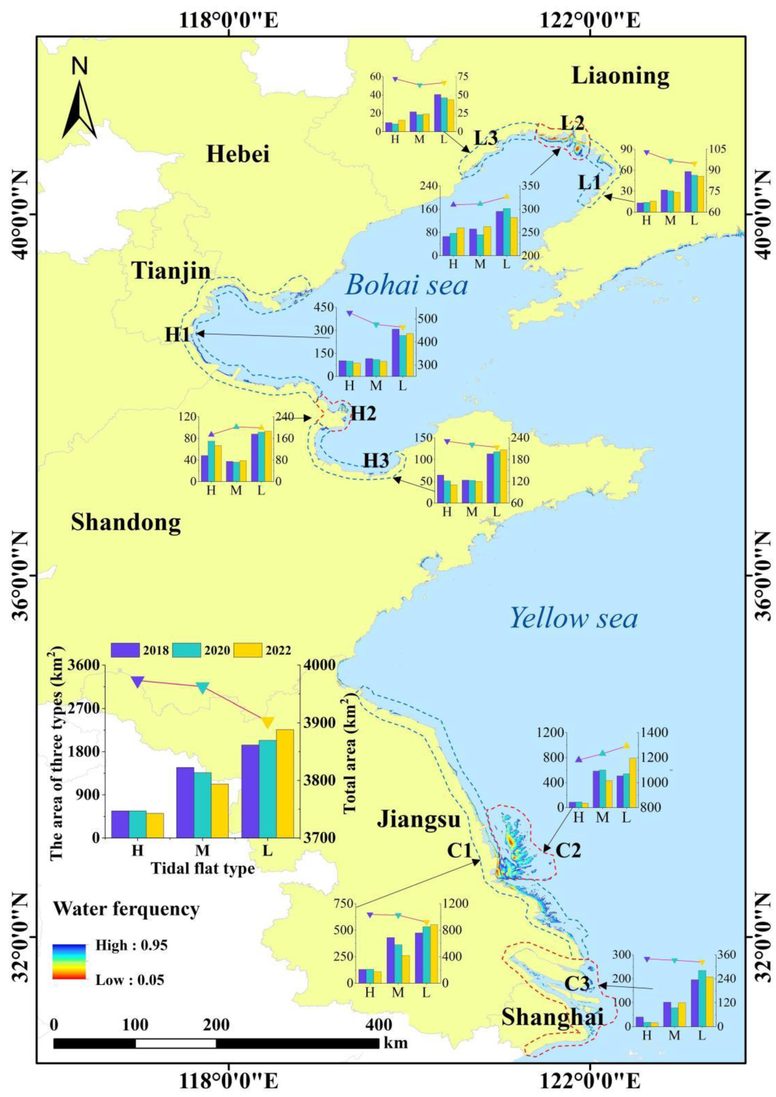
3.2. 2D Changes in Tidal Flats

The total area of the tidal flats of the YBS was 4778.36 km2 in 2022 and is of great spatial variation. Tidal flats were primarily distributed at the edge of the large river deltas, such as the Yangtze River Delta and Yellow River Delta, etc. Jiangsu Province had the most tidal flats among the provinces with a total area of 2279.71 km2, while Tianjin had the least, with only 58.94 km2. The high, middle, and low-tidal flats were 640.08 km2, 1374.28 km2, and 2763 km2 throughout the YBS in 2022, respectively (Figure 6).
Over the period from 2016 to 2022, tidal flats suffered an overall loss in area across nine regions (Figure 7), resulting in a net loss of approximately 70.52 km2, representing 1.79% of the total. The gain and loss in tidal flats area from 2018 to 2022 were 105.25 km2 and 175.78 km2, respectively. The losses in tidal flats area from 2018 to 2022 and from 2020 to 2022 were 10.62 km2 and 59.91 km2, respectively. Figure 7 provides an overview of the changes in tidal flat areas in different regions, revealing the following trends: (1) Regions L2, H2, and C2 exhibited gaining trends. Region C2 experienced the greatest gain over the entire study period, while region L2 had the smallest gain, with gains of 111.25 km2 and 17.09 km2, respectively. (2) In contrast, regions L1, L3, H1, H3, C1, and C3 showed a losing trend in tidal flat areas. Region C1 experienced the highest loss of an area of 115.61 km2, followed by region H1, which lost 62.40 km2. Region C3 experienced the smallest loss, with a loss of only 16.08 km2. Notably, apart from regions C3 and C2, most of the tidal flats near the estuary experienced gain, while the bays and coastal tidal flats further away from the estuary were subjected to loss.

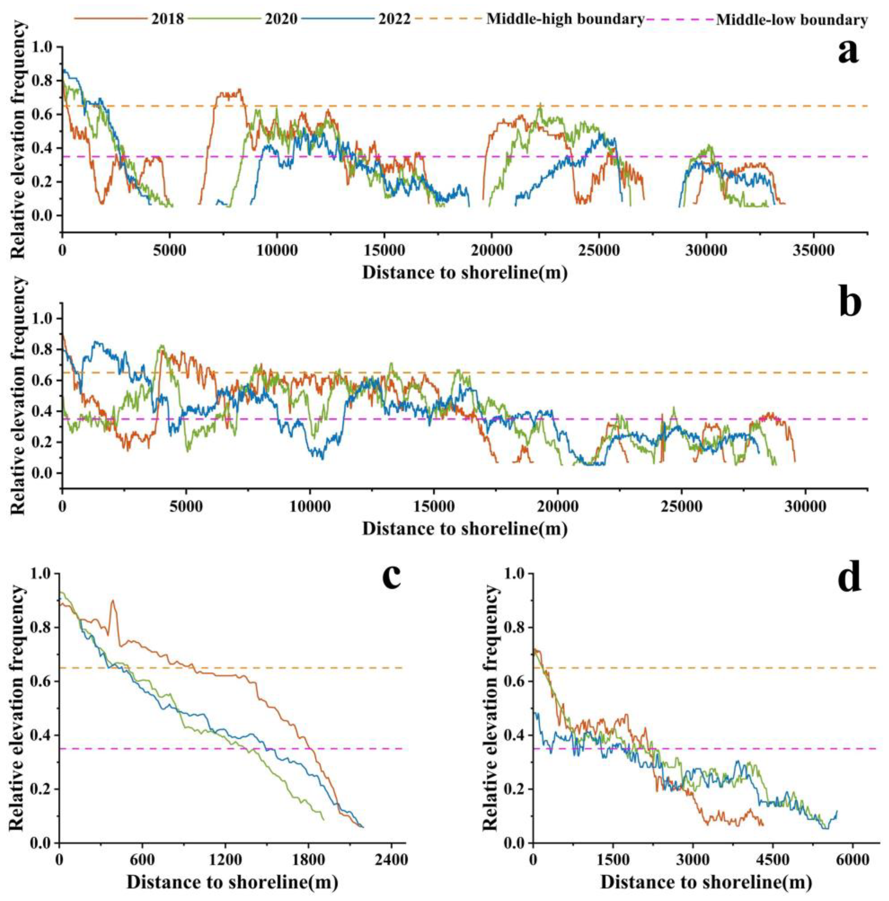
3.3. 3D Changes in Tidal Flats

Considering the high level of variation in tidal ranges in the study area, the 3D morphology of tidal flats was analyzed using the changes in inundation probability to evaluate their vulnerability to the rising sea level. A classification system for tidal flats was defined in our study, including high-tidal flats, mid-tidal flats, and low-tidal flats, with inundation probability from 0.05 to 0.35, 0.35 to 0.65, and 0.65 to 0.95, respectively.
There is an overall erosion trend in the 3D morphology of tidal flats. During the period from 2018 to 2022, the areas of high-tidal flats and mid-tidal flats experienced reductions of 50.24 km2 and 344.13 km2, respectively. In contrast, the area of low-tidal flats increased by 323.85 km2. Among them, the C3 and C2 regions witnessed the most significant decreases in the areas of high-tidal flats and mid-tidal flats, with reductions of 24.37 km2 and 154.23 km2, respectively. Moreover, there were localized areas where the high-tidal flats and mid-tidal flats exhibited increases. The L2 region experienced the most substantial increases, of 29.68 km2 and 8.16 km2, respectively, while H2 had increases of 18.652 and 1.46 km2. Conversely, the low-tidal flat areas exhibited a general growth trend. Among these, the C2 region experienced the most substantial increase, reaching 283.69 km2, followed by C1 and C3 with 76.55 km2 and 11.27 km2, respectively. Some individual areas experienced decreases, such as the H1 region, which decreased by 28.78 km2.
Herein, we also conducted a transect analysis of tidal flats for a detailed illustration of morphological changes (Figure 8). The evolution patterns of tidal flats can be classified into four forms: (1) rapid erosion, where the shoreline retreated more than 500 m inland, and experienced a relative elevation frequency decrease exceeding 20%; (2) slow erosion, where the shoreline receded less than 500 m inland and witnessed a relative elevation frequency decrease of less than 20%; (3) rapid accretion, where the shoreline expanded more than 500 m towards the sea and demonstrated a relative elevation frequency increase exceeding 20%, and (4) gradual accretion, where the shoreline expanded less than 500 m towards the sea and exhibited a relative elevation frequency increase of less than 20%.
The mid- and low-tidal flats decreased simultaneously (Figure 9f,h,i), with a noticeable landward retreat of the lower boundary of tidal flats, indicating rapid erosion. We also found that the mid-tidal flats eroded and transformed into low-tidal flats (Figure 9b–d,g,j,k and Figure 10a), while the low-tidal flats experienced a slight erosion or even slight accretion, with the less pronounced retreat of the tidal flats inward. In Figure 9e, a significant expansion of tidal flats can be observed, while Figure 9a and Figure 10b,d demonstrate a slow accretion in tidal flats. Combining the previous results of the 2D morphology of tidal flats, it can be inferred that the L1, L3, and H1 regions are primarily undergoing rapid erosion, while H3, C1, and C3 are in a state of slow erosion. The pattern of gradual accretion with slow growth dominates the L2 tidal flats. The H2 tidal flats exhibit complex changes, influenced by all four patterns, transitioning from a period of rapid accretion to a period of slow erosion. C2 is mainly characterized by slow erosion. In light of the above analysis, it can be inferred that the elevation of tidal flats in the nine regions is primarily undergoing erosion, with a minority experiencing accretion.

4. Discussion

4.1. Robustness and Uncertainties

In this study, we extensively utilized Landsat and Sentinel-2 images from 2017 to 2022 through the GEE platform. To account for the dynamic changes in tidal inundation, we improved a specialized extraction model for tidal flat wetlands, yielding satisfactory classification results. This can be mainly attributed to three factors. Firstly, the combination of freely available Landsat with Sentinel-2 data has improved the revisit period of the satellites (greater than 2–5 days) and provided higher spatial resolution (10 m). The higher temporal resolution facilitates more frequent capturing of tidal flat information during low-tide and high-tide periods, while the improved spatial resolution of Sentinel-2 enables finer mapping of tidal flats. This is crucial for monitoring the dynamic intertidal wetland environment [55]. Secondly, pixel-based image synthesis reduces the uncertainty caused by tidal variations within the scenes and low-quality observation pixels. Thirdly, the use of appropriate water indices based on the sediment content of different nearshore water bodies has greatly reduced the misclassification and omission of tidal flats. Finally, the utilization of the GEE platform allows for rapid access and parallel processing of thousands of satellite images. This efficient platform facilitates the handling of large volumes of data, enabling timely and effective analysis. Our proposed PITMA method is applicable to other tidal flat areas. Firstly, the method is grounded in principles of physics and geography. It calculates the inundation probability of each pixel in the tidal flat based on the elevation of various regions and the tidal range during the same time period, which are intrinsic attributes of tidal flats. Secondly, our extensive tidal flat dataset spans 7978 km, capturing various tidal flat types and complex water bodies worldwide, and its accuracy has been rigorously validated. Therefore, our method can be easily applied to other tidal flat areas with remote sensing data.
We compared our study with several other datasets of tidal flats, namely the 2018 Chinese Coastal Wetland Map (referred to as FUDAN/OU) [54], the 2020 Chinese Tidal Flat Map (referred to as CTF) [48], and the East Asia Tidal Wetland Map circa 2020 (referred to as MTWN) [56], in terms of area (Figure 11) and spatial distribution (Figure 12). Due to disparities in data sources, methods, and time spans, variations exist among these tidal flat maps. Our tidal flat map covers a larger overall area compared to FUDAN/OU, but a smaller area compared to MTWN. In some regions, CTF shows slightly more extensive tidal flats compared to our study, except in Jiangsu, where it shows smaller extents.
These differences are expected since it relies on only one year of Landsat data. FUDAN/OU misclassifies nearshore tidal flats as seawater [54], leading to an incomplete extraction of tidal flats in their map. In contrast, our study utilizes a combination of two years of Sentinel-2 imagery and Landsat series imagery and uses two indices to classify the land and water with higher accuracy, enabling us to capture finer and more extensive tidal flat features. The slightly larger overall tidal flat extent in CTF is mainly attributed to the use of different spectral indices. CTF utilized NDVI for comprehensive analysis in determining the minimum water area, whereas we employed mNDWI and AWEI to accurately differentiate between tidal flats and water bodies of different turbidity levels. NDVI-MSIC incorrectly classifies some sediment-laden areas as tidal flats (Figure 12(a2)), and misclassifies vegetation as tidal flats (Figure 12(d2)), whereas the more water-sensitive mNDWI accurately distinguishes suspended sediments from tidal flats. Furthermore, in the low-latitude regions, we extracted a larger tidal flats area than CTF (Figure 12(b2,c2)). The utilization of only one and a half years of Sentinel-2 imagery in CTF failed to capture more tidal flat areas. These factors contribute to the discrepancies between our results and CTF. Regarding MTWN, the primary inconsistency lies in the methodology employed. We differentiated tidal flats using a 0.05–0.95 water frequency threshold based on time-series images. In contrast, MTWN employed a random forest method to identify tidal flats and water bodies, and due to spectral similarities, it may have extracted some intertidal mudflats or sandy beaches located above the high tide line (Figure 12(a3,c3)). However, this aspect is not reflected in our results, resulting in smaller extents compared to MTWN.
However, certain objective factors can influence the accuracy of the extraction outcomes. Firstly, the study area has a significant north-south span, with the southern part characterized by a subtropical monsoon climate and frequent cloud cover, which makes it challenging to obtain an adequate quantity of images. Secondly, our research is limited to the exposed tidal flats observed in satellite imagery, and it cannot be determined whether the actual highest and lowest tides can be observed. Lastly, despite employing a frequency-based approach to effectively utilize data from both satellite sources, there may still be a minor presence of cloud pixels on the images even after applying quality assurance (QA) bands for cloud removal [57]. These remaining cloud pixels can potentially affect the precision of our results.

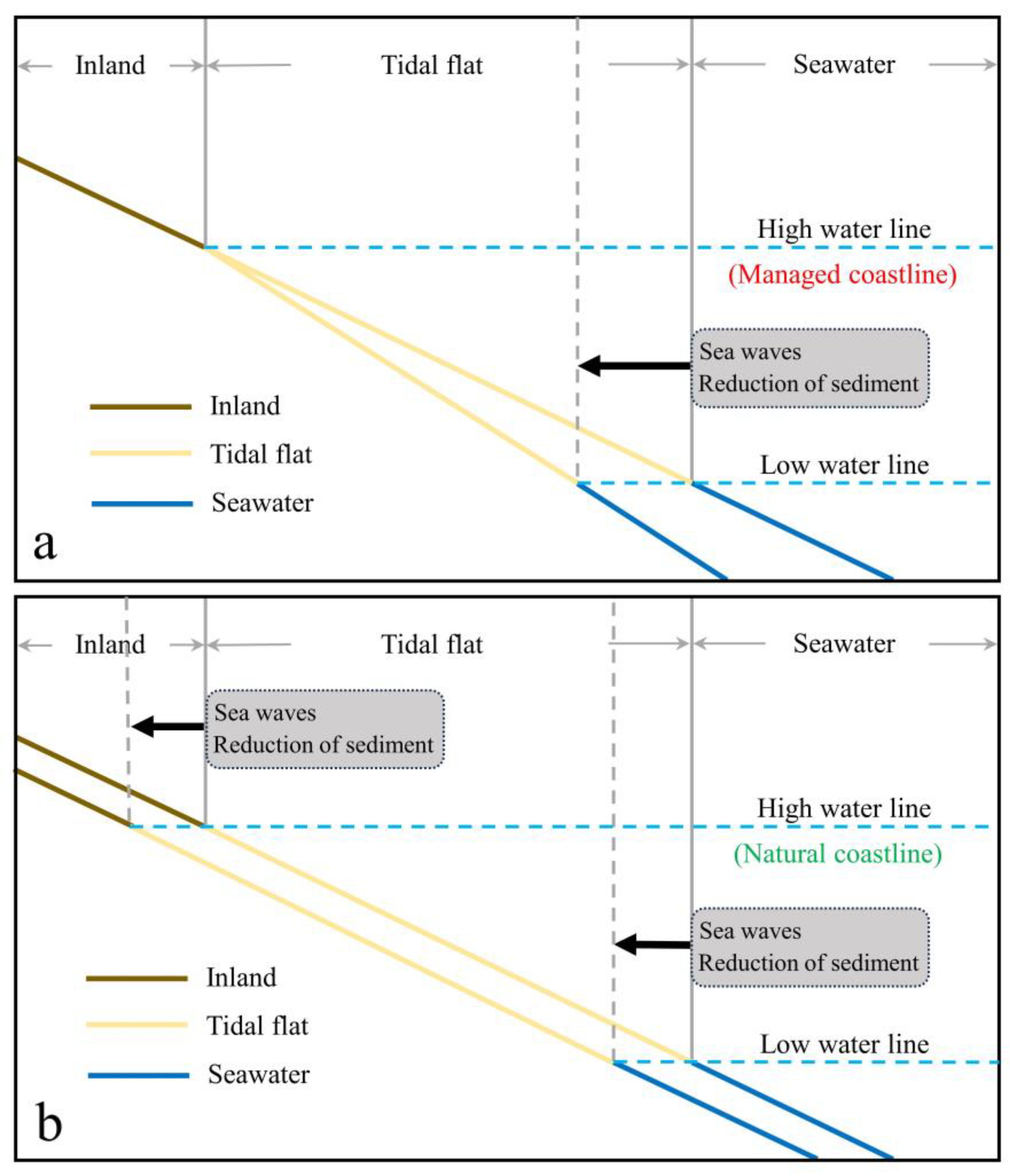
4.2. Drivers of Tidal Flat Dynamics in YBS

4.2.1. Tidal Flat Changes Induced by Sediment

The sediment supply and the distance from the estuary directly or indirectly influence erosion and deposition of tidal flats. Among the rivers that transport freshwater and sediment to the Bohai Sea, the Yellow River exhibits the highest runoff and sediment load, constituting 77.96% and 96.69% of the total, respectively [58]. The dominant current on the western side of the Yellow Sea is the Yellow Sea Coastal Current (YSCC) [59,60]. It originates from the southern part of the Bohai Sea and flows eastward along the northern coast of the Shandong Peninsula via the Dengzhou Waterway (Figure 13). After bypassing Chengshantou, it turns southward and reaches the coast of Jiangsu. On the eastern side, the primary current is the Yellow Sea Warm Current (YSWC). The Yellow Sea Warm Current enters from the northern part of the Bohai Strait and divides into two branches: the northern branch flows eastward along the western coast of the Bohai Sea, generating a cyclonic circulation in Liaodong Bay, and the southern branch enters the Bohai Bay and follows the coast until it exits through the southern part of the Bohai Strait [61,62]. The sediments are transported by these ocean currents to the estuary and its surrounding coastline. However, the construction of numerous reservoirs and water diversion projects has led to a significant decrease in the amount of sediment transported by rivers [19]. The average annual sediment transport of the Yangtze River and Yellow River significantly decreased around the turn of the 21st century. As the transportation of sediment by ocean currents to tidal flats located far from the estuary continues, this will lead to tidal flat erosion closer to the estuary mouth, as sediment import becomes smaller than export (Figure 14a). Our research findings revealed that the loss of tidal flats has occurred in distinct stages over time, encompassing both severe and mild erosion. For instance, in the H1 and H3 regions, sediment from the Yellow River is primarily influenced by the counterclockwise circulation of the southern branch of the Bohai Sea, resulting in its predominant transportation to the H1 area. The H1 region experienced mild erosion due to its greater distance from the river mouth, reduced sediment transport, and wave erosion. The loss of tidal flat wetlands is associated with a gradual reduction in the area of mid-high-tidal flats, which transition to low-tidal flats. In contrast, the H3 region encounters even lower sediment transport, posing challenges for the transportation of sediment from the Yellow River mouth to the northern Bohai Bay area. The loss of tidal flat wetlands in this region is consistent with the overall decrease in the frequency of relative elevation. Profile change diagrams also illustrate a significant reduction in the width of the entire tidal flat, indicating a noticeable retreat inland. Importantly, if the supply of sediment remains inadequate, mild erosion may progress towards severe erosion, resulting in the eventual disappearance of low-tidal flats due to ongoing wave erosion. From an alternative standpoint, tidal flat erosion can be classified into two scenarios: managed coastlines (Figure 14a) and natural coastlines (Figure 14b). In managed coastlines, human activities maintain the high-tidal flats, while the mid- and low-tidal flats shift landward due to reduced sediment supply, resulting in an overall reduction in tidal flat width. Conversely, in natural coastlines, the high and low water lines move inland due to reduced sediment transport and wave action. However, the overall area of the tidal flats does not undergo significant changes.
Although the tidal flat area has generally decreased in the aforementioned regions, there have been periods of increase in tidal flat wetland areas throughout the time series. In the case of H2, the diversion of the Yellow River northward in 1996 resulted in the loss of its primary sediment supply to the southern region of the estuary [63]. Consequently, the tidal flats in the region have experienced a gradual erosion process. However, their proximity to the river mouth and the impact of tidal currents have resulted in reduced erosion rates over time, as sediment transport to the southern delta has played a mitigating role. The tidal flats in the northern region have exhibited a trend of northward expansion, albeit at a decelerated growth rate, attributed to the prolonged decline in sediment supply. Sediment has experienced a decline in recent years, increasing from an average of 152 million tons (2017–2018) to 292 million tons (2019–2020), and then decreasing to 184 million tons (Figure 15b). Throughout this entire period, the overall area of tidal flats has displayed a substantial increase, transitioning to a slightly diminished state, consequently leading to a reduction in the extent of high-tidal flats. Similarly, in the C2 region, the RSRS has experienced an overall expansion in the total area of tidal flats. However, the area of mid- to high-tidal flats has consistently declined, while only the low-tidal flats have shown an increase. This situation presents a relatively complex scenario. The sediments primarily originate from the submerged delta of the former Yellow River, which was redirected northward to Shandong and emptied into the sea in 1855, in addition to the Huai and Yangtze Rivers’ discharge [59]. The YSCC (Figure 13) transports sediments from the sandbar located in the abandoned Yellow River delta to the south along the coastline [64] and acts as a protective barrier against erosion for the radiating sand shoal and the northwest coast. However, over time (from 1855 to the present), the former Yellow River delta has been gradually diminishing, leading to a decrease in suspended sediment [65]. The YSCC acts as a powerful force, propelling the radiating sand shoal from the northwest to the southeast, resulting in the gradual erosion of mid-high-tidal flats and even low-tidal flats in the northern part of C2. The remaining water currents disperse across the nearshore tidal channels and small sand ridges, generating residual currents and eddies that persistently transport sediment toward the southeast [66]. This process leads to the erosion of internal sediment and the conversion of mid-high-tidal flats. The tidal flats undergo a gradual process of flattening, giving the impression of sedimentation in terms of their area. However, in reality, they may be undergoing erosion.

4.2.2. Tidal Flat Changes Induced by Vegetation

Coastal vegetation expansion plays a significant role in specific areas. Our six-year time series analysis of relative elevation frequencies of tidal flats has revealed the direct impact of vegetation growth on the expansion or reduction of tidal flats in specific wetland systems. The energy transferred to high-tidal flats by waves is limited, creating favorable conditions for the ongoing growth of new vegetation and sediment stabilization, which establishes suitable boundary conditions for vegetation survival. Observation of C3, situated at the estuary, reveals continuous sediment accumulation in this region, resulting in the outward expansion of tidal flat boundaries, despite the overall area exhibiting a declining trend. This expansion is attributed to vegetation encroaching directly upon the survival space of the high-tidal flats [67], covering an area of 88.60 km2 (Figure 16). There seems to be a correlation between the vegetation increase and sediment transport. Over the three periods of 2018, 2020, and 2022, the total sediment transport increased from 187.1 million tons to 269 million tons and then decreased to 168.5 million tons (Figure 15b), while the increase in vegetation area decreased from 62.89 km2 to 25.71 km2. Thus, while the expansion of vegetation encroaches directly upon the tidal flat area, the reduction in sediment transport hinders the rapid accumulation of sediment in the high-tidal flats to meet the conditions for vegetation survival, thereby limiting further vegetation expansion.

5. Conclusions

Our study proposed a PMITMA algorithm for mapping coastal tidal flats, which integrates multi-source time-series satellite imagery and utilizes muti-indices for water index calculation, along with the K-Means++ method for water-land separation. This model effectively addresses challenges related to tides, waves, and cloud contamination. Consequently, it generates highly detailed maps of tidal flat coverage along the coastlines of the Yellow and Bohai Seas from 2017 to 2022. These maps offer robust data support for the scientific management and utilization of coastal tidal flat resources while facilitating high-quality development in the coastal zone.
Our research findings indicate a shift in the causes of tidal flat changes, from previous human reclamation to sediment transport and vegetation growth. In specific regions, such as the Yangtze River delta, the expansion of vegetation covers an area of 88.60 km2, while sediment from the Yellow River and Yangtze River decreased by 81.33% and 60.80%, respectively, during the transition from the twentieth to the twenty-first century. Over the study period, the tidal flat area in the YBS decreased by 78 km2, resulting in a current total area of 4778.32 km2. The primary change pattern entailed a conversion from mid-high-tidal flats to low-tidal flats, along with the loss of pre-existing low-tidal flats. The most affected areas by these losses were the bays and coastal segments distant from river mouths.

Author Contributions

Conception, W.W.; Methodology, Z.G. and W.W.; Validation, Z.G.; Data Curation, Z.G. and S.G.; Writing—original draft, Z.G.; Writing—review and editing, C.C., H.Z., H.S., Y.H. and W.W.; Funding Acquisition, W.W. All authors have read and agreed to the published version of the manuscript.

Funding

This research was funded by the National Natural Science Foundation of China (Grant No. 42301540), the Open Research Fund of State Key Laboratory of Estuarine and Coastal Research (Grant number SKLEC-KF202307), the Natural Science Foundation of Fujian Province (Grant No. 2022J05024), the Education Department of Fujian Province (Grant No. JAT210027), and the Natural Science Foundation for Distinguished Young Scholars of Fujian Province, China (Grant No. 2021J06014).

Data Availability Statement

The data presented in this study are available on request from the corresponding author.

Acknowledgments

We appreciate the critical and constructive comments and suggestions from the reviewers that helped improve the quality of this manuscript.

Conflicts of Interest

The authors declare no conflicts of interest.

References

  1. Dyer, K.R.; Christie, M.C.; Wright, E.W. The classification of intertidal mudflats. Cont. Shelf Res. 2000, 20, 1039–1060. [Google Scholar] [CrossRef]
  2. Murray, N.J.; Phinn, S.R.; Clemens, R.S.; Roelfsema, C.M.; Fuller, R.A. Continental Scale Mapping of Tidal Flats across East Asia Using the Landsat Archive. Remote Sens. 2012, 4, 3417–3426. [Google Scholar] [CrossRef]
  3. Ma, Z.; Melville, D.S.; Liu, J.; Chen, Y.; Yang, H.; Ren, W.; Zhang, Z.; Piersma, T.; Li, B. Rethinking China’s new great wall. Science 2014, 346, 912–914. [Google Scholar] [CrossRef]
  4. Solomon, S.; Plattner, G.-K.; Knutti, R.; Friedlingstein, P. Irreversible climate change due to carbon dioxide emissions. Proc. Natl. Acad. Sci. USA 2009, 106, 1704–1709. [Google Scholar] [CrossRef]
  5. Rodriguez, J.F.; Saco, P.M.; Sandi, S.; Saintilan, N.; Riccardi, G. Potential increase in coastal wetland vulnerability to sea-level rise suggested by considering hydrodynamic attenuation effects. Nat. Commun. 2017, 8, 16094. [Google Scholar] [CrossRef]
  6. Dhanjal-Adams, K.L.; Hanson, J.O.; Murray, N.J.; Phinn, S.R.; Wingate, V.R.; Mustin, K.; Lee, J.R.; Allan, J.R.; Cappadonna, J.L.; Studds, C.E.; et al. The distribution and protection of intertidal habitats in Australia. Emu Austral Ornithol. 2016, 116, 208–214. [Google Scholar] [CrossRef]
  7. Phinn, S.R.; Kovacs, E.M.; Roelfsema, C.M.; Canto, R.F.; Collier, C.J.; McKenzie, L.J. Assessing the potential for satellite image monitoring of seagrass thermal dynamics: For inter- and shallow sub-tidal seagrasses in the inshore Great Barrier Reef World Heritage Area, Australia. Int. J. Digit. Earth 2018, 11, 803–824. [Google Scholar] [CrossRef]
  8. Ghosh, S.; Mishra, D.R.; Gitelson, A.A. Long-term monitoring of biophysical characteristics of tidal wetlands in the northern Gulf of Mexico—A methodological approach using MODIS. Remote Sens. Environ. 2016, 173, 39–58. [Google Scholar] [CrossRef]
  9. Murray, N.J.; Phinn, S.R.; DeWitt, M.; Ferrari, R.; Johnston, R.; Lyons, M.B.; Clinton, N.; Thau, D.; Fuller, R.A. The global distribution and trajectory of tidal flats. Nature 2019, 565, 222–225. [Google Scholar] [CrossRef]
  10. McGranahan, G.; Balk, D.; Anderson, B. The rising tide: Assessing the risks of climate change and human settlements in low elevation coastal zones. Environ. Urban. 2007, 19, 17–37. [Google Scholar] [CrossRef]
  11. Sengupta, D.; Chen, R.; Meadows, M.E.; Choi, Y.R.; Banerjee, A.; Zilong, X. Mapping Trajectories of Coastal Land Reclamation in Nine Deltaic Megacities using Google Earth Engine. Remote Sens. 2019, 11, 2621. [Google Scholar] [CrossRef]
  12. Wu, W.; Gao, Y.; Chen, C.; Sun, Y.; Su, H. A Framework for Assessing the Dynamic Coastlines Induced by Urbanization Using Remote Sensing Data: A Case Study in Fujian, China. Remote Sens. 2022, 14, 2911. [Google Scholar] [CrossRef]
  13. Ren, C.; Wang, Z.; Zhang, Y.; Zhang, B.; Chen, L.; Xi, Y.; Xiao, X.; Doughty, R.B.; Liu, M.; Jia, M.; et al. Rapid expansion of coastal aquaculture ponds in China from Landsat observations during 1984–2016. Int. J. Appl. Earth Obs. Geoinf. 2019, 82, 101902. [Google Scholar] [CrossRef]
  14. Jung, P.S.; Seo, H.-J.; Min, P.S.; Park, S.-H.; Ahn, I.J.; Seo, K.S. The Analysis of Coastal Erosion and Erosion Impact Assessment in the East Coast. J. Korean Soc. Coast. Ocean Eng. 2021, 33, 246–256. [Google Scholar] [CrossRef]
  15. Beeharry, Y.D.; Bekaroo, G.; Bokhoree, C.; Phillips, M.R. Impacts of sea-level rise on coastal zones of Mauritius: Insights following calculation of a coastal vulnerability index. Nat. Hazards 2022, 114, 27–55. [Google Scholar] [CrossRef]
  16. Lovelock, C.E.; Feller, I.C.; Reef, R.; Hickey, S.; Ball, M.C. Mangrove dieback during fluctuating sea levels. Sci. Rep. 2017, 7, 1680. [Google Scholar] [CrossRef]
  17. Yim, J.; Kwon, B.-O.; Nam, J.; Hwang, J.H.; Choi, K.; Khim, J.S. Analysis of forty years long changes in coastal land use and land cover of the Yellow Sea: The gains or losses in ecosystem services. Environ. Pollut. 2018, 241, 74–84. [Google Scholar] [CrossRef]
  18. Mentaschi, L.; Vousdoukas, M.I.; Pekel, J.-F.; Voukouvalas, E.; Feyen, L.J.S.R. Global long-term observations of coastal erosion and accretion. Sci. Rep. 2018, 8, 12876. [Google Scholar] [CrossRef]
  19. Dethier, E.N.; Renshaw, C.E.; Magilligan, F.J.J.S. Rapid changes to global river suspended sediment flux by humans. Science 2022, 376, 1447–1452. [Google Scholar] [CrossRef]
  20. Wu, W.; Zhi, C.; Gao, Y.; Chen, C.; Chen, Z.; Su, H.; Lu, W.; Tian, B. Increasing fragmentation and squeezing of coastal wetlands: Status, drivers, and sustainable protection from the perspective of remote sensing. Sci. Total Environ. 2022, 811, 152339. [Google Scholar] [CrossRef]
  21. Pari, Y.; Murthy, M.R.; Subramanian, B.; Ramachandran, S. Morphological changes at Vellar estuary, India—Impact of the December 2004 tsunami. J. Environ. Manag. 2008, 89, 45–57. [Google Scholar] [CrossRef]
  22. Chen, B.; Yang, Y.; Wen, H.; Ruan, H.; Zhou, Z.; Luo, K.; Zhong, F. High-resolution monitoring of beach topography and its change using unmanned aerial vehicle imagery. Ocean Coast. Manag. 2018, 160, 103–116. [Google Scholar] [CrossRef]
  23. Zhang, H.; Wang, L.; Zhao, Y.; Cao, J.; Xu, M. Application of Airborne LiDAR Measurements to the Topographic Survey of the Tidal Flats of the Northern Jiangsu Radial Sand Ridges in the Southern Yellow Sea. Front. Mar. Sci. 2022, 9, 871156. [Google Scholar] [CrossRef]
  24. Mason, D.C.; Davenport, I.J.; Robinson, G.J.H.; Flather, R.A.; McCartney, B.S. Construction of an Inter-Tidal Digital Elevation Model by the Water-Line Method. Geophys. Res. Lett. 1995, 22, 3187–3190. [Google Scholar] [CrossRef]
  25. Salameh, E.; Frappart, F.; Turki, I.; Laignel, B. Intertidal topography mapping using the waterline method from Sentinel-1 &-2 images: The examples of Arcachon and Veys Bays in France. ISPRS J. Photogramm. Remote Sens. 2020, 163, 98–120. [Google Scholar] [CrossRef]
  26. Zhang, S.; Xu, Q.; Wang, H.; Kang, Y.; Li, X. Automatic Waterline Extraction and Topographic Mapping of Tidal Flats From SAR Images Based on Deep Learning. Geophys. Res. Lett. 2022, 49, e2021GL096007. [Google Scholar] [CrossRef]
  27. Ryu, J.-H.; Kim, C.-H.; Lee, Y.-K.; Won, J.-S.; Chun, S.-S.; Lee, S. Detecting the intertidal morphologic change using satellite data. Estuar. Coast. Shelf Sci. 2008, 78, 623–632. [Google Scholar] [CrossRef]
  28. Chen, L.C.; Rau, J.Y. Detection of shoreline changes for tideland areas using multi-temporal satellite images. Int. J. Remote Sens. 1998, 19, 3383–3397. [Google Scholar] [CrossRef]
  29. Chang, M.; Li, P.; Li, Z.; Wang, H. Mapping Tidal Flats of the Bohai and Yellow Seas Using Time Series Sentinel-2 Images and Google Earth Engine. Remote Sens. 2022, 14, 1789. [Google Scholar] [CrossRef]
  30. Chen, C.; Zhang, C.; Tian, B.; Wu, W.; Zhou, Y. Tide2Topo: A new method for mapping intertidal topography accurately in complex estuaries and bays with time-series Sentinel-2 images. ISPRS J. Photogramm. Remote Sens. 2023, 200, 55–72. [Google Scholar] [CrossRef]
  31. Wu, W.; Zhang, M.; Chen, C.; Chen, Z.; Yang, H.; Su, H. Coastal reclamation shaped narrower and steeper tidal flats in Fujian, China: Evidence from time-series satellite data. Ocean Coast. Manag. 2024, 247, 106933. [Google Scholar] [CrossRef]
  32. Sagar, S.; Roberts, D.; Bala, B.; Lymburner, L. Extracting the intertidal extent and topography of the Australian coastline from a 28 year time series of Landsat observations. Remote Sens. Environ. 2017, 195, 153–169. [Google Scholar] [CrossRef]
  33. Mao, D.; Liu, M.; Wang, Z.; Li, L.; Man, W.; Jia, M.; Zhang, Y. Rapid Invasion of Spartina Alterniflora in the Coastal Zone of Mainland China: Spatiotemporal Patterns and Human Prevention. Sensors 2019, 19, 2308. [Google Scholar] [CrossRef]
  34. MacKinnon, J.; Verkuil, Y.I.; Murray, N. IUCN Situation Analysis on East and Southeast Asian Intertidal Habitats, with Particular Reference to the Yellow Sea (Including the Bohai Sea); Occasional Paper of the IUCN Species Survival Commission no. 47; IUCN: Gland, Switzerland, 2012. [Google Scholar]
  35. Wei, Y.; Jiao, J.; Zhao, G.; Zhao, H.; He, Z.; Mu, X.J.C. Spatial–temporal variation and periodic change in streamflow and suspended sediment discharge along the mainstream of the Yellow River during 1950–2013. Catena 2016, 140, 105–115. [Google Scholar] [CrossRef]
  36. Qiao, S.; Shi, X.; Wang, G.; Zhou, L.; Hu, B.; Hu, L.; Yang, G.; Liu, Y.; Yao, Z.; Liu, S. Sediment accumulation and budget in the Bohai sea, Yellow Sea and East China sea. Mar. Geol. 2017, 390, 270–281. [Google Scholar] [CrossRef]
  37. Zhou, Z.; Bian, C.; Chen, S.; Li, Z.; Jiang, W.; Wang, T.; Bi, R. Sediment concentration variations in the East China Seas over multiple timescales indicated by satellite observations. J. Mar. Syst. 2020, 212, 103430. [Google Scholar] [CrossRef]
  38. Wang, S.; Mao, Y.; Zheng, L.; Qiu, Z.; Bilal, M.; Sun, D. Remote sensing of water turbidity in the Eastern China Seas from Geostationary Ocean Colour Imager. Int. J. Remote Sens. 2020, 41, 4080–4101. [Google Scholar] [CrossRef]
  39. Xu, H. Development of remote sensing water indices:a review. J. Fuzhou Univ. Nat. Sci. Ed. 2021, 49, 613–625. [Google Scholar]
  40. McFeeters, S.K. The use of the normalized difference water index (NDWI) in the delineation of open water features. Int. J. Remote Sens. 1996, 17, 1425–1432. [Google Scholar] [CrossRef]
  41. Xu, H. Modification of normalised difference water index (NDWI) to enhance open water features in remotely sensed imagery. Int. J. Remote Sens. 2006, 27, 3025–3033. [Google Scholar] [CrossRef]
  42. Feyisa, G.L.; Meilby, H.; Fensholt, R.; Proud, S.R. Automated Water Extraction Index: A new technique for surface water mapping using Landsat imagery. Remote Sens. Environ. 2014, 140, 23–35. [Google Scholar] [CrossRef]
  43. Singh, K.V.; Setia, R.; Sahoo, S.; Prasad, A.; Pateriya, B. Evaluation of NDWI and MNDWI for assessment of waterlogging by integrating digital elevation model and groundwater level. Geocarto Int. 2015, 30, 650–661. [Google Scholar] [CrossRef]
  44. Acharya, T.D.; Subedi, A.; Lee, D.H. Evaluation of Water Indices for Surface Water Extraction in a Landsat 8 Scene of Nepal. Sensors 2018, 18, 2580. [Google Scholar] [CrossRef]
  45. Fisher, A.; Flood, N.; Danaher, T. Comparing Landsat water index methods for automated water classification in eastern Australia. Remote Sens. Environ. 2016, 175, 167–182. [Google Scholar] [CrossRef]
  46. Nguyen, U.N.T.; Pham, L.T.H.; Dang, T.D. an automatic water detection approach using Landsat 8 OLI and Google earth engine cloud computing to map lakes and reservoirs in New Zealand. Environ. Monit. Assess. 2020, 192, 616. [Google Scholar] [CrossRef]
  47. Yang, Y.; Liu, Y.; Zhou, M.; Zhang, S.; Zhan, W.; Sun, C.; Duan, Y. Landsat 8 OLI image based terrestrial water extraction from heterogeneous backgrounds using a reflectance homogenization approach. Remote Sens. Environ. 2015, 171, 14–32. [Google Scholar] [CrossRef]
  48. Jia, M.; Wang, Z.; Mao, D.; Ren, C.; Wang, C.; Wang, Y. Rapid, robust, and automated mapping of tidal flats in China using time series Sentinel-2 images and Google Earth Engine. Remote Sens. Environ. 2021, 255, 112285. [Google Scholar] [CrossRef]
  49. Sunder, S.; Ramsankaran, R.; Ramakrishnan, B. Inter-comparison of remote sensing sensing-based shoreline mapping techniques at different coastal stretches of India. Environ. Monit. Assess. 2017, 189, 290. [Google Scholar] [CrossRef]
  50. Le Hung, T.; Thi Giang, L.; Van Hoan, K.; Thi Minh Ly, T.; Thi Thu Nga, N. Application of remote sensing technique for shoreline change detection in Ninh Binh and Nam Dinh provinces (Vietnam) during the period 1988 to 2018 based on water indices. Russ. J. Earth Sci. 2020, 20, ES2004. [Google Scholar] [CrossRef]
  51. Huang, C.; Chen, Y.; Zhang, S.; Wu, J. Detecting, Extracting, and Monitoring Surface Water From Space Using Optical Sensors: A Review. Rev. Geophys. 2018, 56, 333–360. [Google Scholar] [CrossRef]
  52. Li, D.; Wu, B.; Chen, B.; Xue, Y.; Zhang, Y. Review of water body information extraction based on satellite remote sensing. J. Tsinghua Univ. Sci. Technol. 2020, 60, 147–161. [Google Scholar] [CrossRef]
  53. Arthur, D.; Vassilvitskii, S. k-means++: The advantages of careful seeding. In Proceedings of the Eighteenth Annual ACM-SIAM Symposium on Discrete Algorithms, New Orleans, LO, USA, 7–9 January 2007; pp. 1027–1035. [Google Scholar]
  54. Wang, X.; Xiao, X.; Zou, Z.; Hou, L.; Qin, Y.; Dong, J.; Doughty, R.B.; Chen, B.; Zhang, X.; Chen, Y.; et al. Mapping coastal wetlands of China using time series Landsat images in 2018 and Google Earth Engine. ISPRS J. Photogramm. Remote Sens. 2020, 163, 312–326. [Google Scholar] [CrossRef]
  55. Wu, W.; Zhi, C.; Chen, C.; Tian, B.; Chen, Z.; Su, H. Detecting annual anthropogenic encroachment on intertidal vegetation using full Landsat time-series in Fujian, China. GIScience Remote Sens. 2022, 59, 2266–2282. [Google Scholar] [CrossRef]
  56. Zhang, Z.; Xu, N.; Li, Y.; Li, Y. Sub-continental-scale mapping of tidal wetland composition for East Asia: A novel algorithm integrating satellite tide-level and phenological features. Remote Sens. Environ. 2022, 269, 112799. [Google Scholar] [CrossRef]
  57. Dong, J.; Xiao, X.; Menarguez, M.A.; Zhang, G.; Qin, Y.; Thau, D.; Biradar, C.; Moore, B., III. Mapping paddy rice planting area in northeastern Asia with Landsat 8 images, phenology-based algorithm and Google Earth Engine. Remote Sens. Environ. 2016, 185, 142–154. [Google Scholar] [CrossRef]
  58. Wang, H.; Wang, A.; Bi, N.; Zeng, X.; Xiao, H. Seasonal distribution of suspended sediment in the Bohai Sea, China. Cont. Shelf Res. 2014, 90, 17–32. [Google Scholar] [CrossRef]
  59. Su, M.; Yao, P.; Wang, Z.B.; Zhang, C.K.; Stive, M.J.F. Exploratory morphodynamic modeling of the evolution of the Jiangsu coast, China, since 1855: Contributions of old Yellow River-derived sediment. Mar. Geol. 2017, 390, 306–320. [Google Scholar] [CrossRef]
  60. Liu, J.; Saito, Y.; Kong, X.; Wang, H.; Xiang, L.; Wen, C.; Nakashima, R. Sedimentary record of environmental evolution off the Yangtze River estuary, East China Sea, during the last similar to 13,000 years, with special reference to the influence of the Yellow River on the Yangtze River delta during the last 600 years. Quat. Sci. Rev. 2010, 29, 2424–2438. [Google Scholar] [CrossRef]
  61. Zheng, Q.; Fang, G.; Song, Y.T. Introduction to special section: Dynamics and circulation of the Yellow, East, and South China Seas. J. Geophys. Res. 2006, 111, C11S01. [Google Scholar] [CrossRef]
  62. Wang, A.; Wang, H.; Bi, N.; Wu, X. Sediment transport and dispersal pattern from the Bohai Sea to the Yellow Sea. J. Coast. Res. 2016, 74, 104–116. [Google Scholar] [CrossRef]
  63. Xu, H.; Jia, A.; Song, X.; Bai, Y. Extraction and spatiotemporal evolution analysis of tidal flats in the Bohai Rim during 1984-2019 based on remote sensing. J. Geogr. Sci. 2023, 33, 76–98. [Google Scholar] [CrossRef]
  64. Kim, W.; Doh, S.-J.; Yu, Y.; Lee, Y.I. Magnetic evaluation of sediment provenance in the northern East China Sea using fuzzy c-means cluster analysis. Mar. Geol. 2013, 337, 9–19. [Google Scholar] [CrossRef]
  65. Wang, Y.; Liu, Y.; Jin, S.; Sun, C.; Wei, X. Evolution of the topography of tidal flats and sandbanks along the Jiangsu coast from 1973 to 2016 observed from satellites. ISPRS J. Photogramm. Remote Sens. 2019, 150, 27–43. [Google Scholar] [CrossRef]
  66. Ni, W.; Wang, Y.; Zou, X.; Zhang, J.; Gao, J. Sediment dynamics in an offshore tidal channel in the southern Yellow Sea. Int. J. Sediment Res. 2014, 29, 246–259. [Google Scholar] [CrossRef]
  67. Wu, W.-T.; Zhou, Y.-X.; Tian, B.J.O.; Management, C. Coastal wetlands facing climate change and anthropogenic activities: A remote sensing analysis and modelling application. Ocean. Coast. Manag. 2017, 138, 1–10. [Google Scholar] [CrossRef]
Figure 1. Geographical setting of the study area. (a) Location of the study area and water indices used on different shorelines. (b) The number of satellite images and the distribution of observation pixels.
Remotesensing 16 00886 g001
Figure 2. Workflow for mapping tidal flats.
Remotesensing 16 00886 g002
Figure 3. Comparison of water index characteristics between tidal flat and water body. (a1) NDWI in Yangtze River Estuary, (a2) mNDWI in Yangtze River Estuary, (a3) AWEI in Yangtze River Estuary, (b1) NDWI in Yellow River Estuary, (b2) mNDWI in Yellow River Estuary, (b3) AWEI in Yellow River Estuary.
Remotesensing 16 00886 g003
Figure 4. Illustration of workflow with case site in the Nanhui tidal flats of the Yangtze Estuary. (a) Satellite images, (b) mNDWI Water Index, (c) K-means++ classification and geographic landmarks, (d) water-land binary image, (e) water frequency, and (f) relative elevation.
Remotesensing 16 00886 g004
Figure 5. Correlation between the relative elevation frequency of tidal flats and ICESAT-2 data. (a) Liaohe Estuary, (b) Diaokou River Estuary, (c) radial sand ridges (RSRS) in Jiangsu middle coast, (d) Jiuduan sands, and (e) Nanhui Beach.
Remotesensing 16 00886 g005
Figure 6. The spatial distribution coverage and areas of the three types of tidal flats along the coast of the Bohai and Yellow Seas in 2022. Subfigures show tidal flats in (a) the Jiangsu middle coast radial sand, (b) Liao River Estuary, (c) Bohai Bay, (d) Yellow River Estuary, (e) the Jiangsu middle coast, and (f) Yangtze River Estuary.
Remotesensing 16 00886 g006
Figure 7. The tidal flat locations of different regions. Starting from the northeastern coastline and heading south, the sections are identified as L1, L2, L3, H1, H2, H3, C1, C2, and C3.
Remotesensing 16 00886 g007
Figure 8. The profile of different regions. (a) Profile lines in the Liao River Estuary, (b,c) profile lines in the Bohai Bay, (d) profiles lines in the Yellow River Estuary, (e) profile line in the Laizhou Bay, (fh) profile lines in the central-northern coastal section of Jiangsu, (i) profile line in the Chongming east beach, and (j) profile line in the Jiuduansha sandbank.
Remotesensing 16 00886 g008
Figure 9. The morphological changes in transects over the study period. (a) Represents the profile line of “1” in Figure 8, (b) represents the profile line of “2” in Figure 8, (c) represents the profile line of “3” in Figure 8, (d) represents the profile line of “4” in Figure 8, (e) represents the profile line of “5” in Figure 8, (f) represents the profile line of “6” in Figure 8, (g) represents the profile line of “7” in Figure 8, (h) represents the profile line of “8” in Figure 8, (i) represents the profile line of “9” in Figure 8, and (j) represents the profile line of “10” in Figure 8, (k) represents the profile line of “11” in Figure 8.
Remotesensing 16 00886 g009
Figure 10. The profile plots of RSRS are drawn based on the positions of the profile lines. (a) Represents the profile line of “12” in Figure 8, (b) represents the profile line of “13” in Figure 8, (c) represents the profile line of “14” in Figure 8, and (d) represents the profile line of “15” in Figure 8.
Remotesensing 16 00886 g010
Figure 11. Comparisons of tidal flat areas with other results, including MTWN, CTF, and FUDAN/OU.
Remotesensing 16 00886 g011
Figure 12. Comparison of the tidal flat extent in our study (No. 1), Jia’s study (CTF) (No. 2), and Zhang’s study (MTWN) (No. 3) in (a1a3) Bohai Bay, (b1b3) Wulei Island Bay, (c1c3) Dingzi Port, and (d1d3) Chongming east tidal flat.
Remotesensing 16 00886 g012
Figure 13. Submarine bathymetry and circulation distribution in the Yellow and Bohai Seas. (YSWC) Yellow Sea Warm Current, (YSCC) Yellow Sea Coastal Current, (ZFCC) Zhejiang and Fujian Coastal Current. The bathymetry is from NOAA National Centers for Environmental Information. 2022: ETOPO 2022 15 Arc-Second Global Relief Model.
Remotesensing 16 00886 g013
Figure 14. Two forms of tidal flat erosion. (a) The form of managed coastline erosion, and (b) the form of natural coastline erosion.
Remotesensing 16 00886 g014
Figure 15. Sediment transport of major rivers. (a) The average sediment transport of rivers during the early 21st century, and (b) sediment transport of major rivers in the past twenty years.
Remotesensing 16 00886 g015
Figure 16. The changes in tidal flats and vegetation in the Yangtze River Estuary from 2018 to 2022. (a) The northern portion of Chongming East Beach, (b) the southern portion of Hengduan Sands, and (c) the eastern portion of Nanhui Beach.
Remotesensing 16 00886 g016
Table 1. The spectral indices used in this study.
IndexTidal Height (cm)
Normalized Difference Water
Index (NDWI)
ρ G r e e n ρ N I R ρ G r e e n + ρ N I R
Modified Normalized Difference Water Index (mNDWI) ρ G r e e n ρ S W I R ρ G r e e n + ρ S W I R
Automated Water Extraction
Index (AWEI)
ρ B l u e + 2.5     ρ G r e e n 1.5 ρ N I R + ρ S W I R 1 0.25 ρ S W I R 2
Normalized Difference
Vegetation Index (NDVI)
ρ N I R ρ R e d ρ N I R + ρ R e d
Table 2. Accuracy of tidal flats map.
PeriodClassTidal FlatsNon-Tidal FlatUA (%)OA (%)
2018Tidal flats36079597.4395.77
Non-tidal flat197301293.86
PA (%)94.8296.94
F1_Score96.1095.37
2020Tidal flats375511097.1595.83
Non-tidal flat185302594.23
PA (%)95.3096.80
F1_Score96.2195.49
2022Tidal flats37378197.8795.60
Non-tidal flat235313293.02
PA (%)94.0897.47
F1_Score95.9395.19
Note: PA is producer’s accuracy; UA is user’s accuracy; OA is overall accuracy.
Disclaimer/Publisher’s Note: The statements, opinions and data contained in all publications are solely those of the individual author(s) and contributor(s) and not of MDPI and/or the editor(s). MDPI and/or the editor(s) disclaim responsibility for any injury to people or property resulting from any ideas, methods, instructions or products referred to in the content.

