1. Introduction
Internal solitary waves in the ocean are captivating phenomena within the field of oceanography, occurring beneath the ocean’s surface and widely present in stably stratified oceans [
1,
2]. With amplitudes reaching up to 240 m [
3], these waves carry substantial energy and have significant impacts on offshore drilling operations [
4,
5]. Simultaneously, they play a crucial role in the intricate interplay of energy within the marine ecosystem [
6]. Hence, it is imperative to precisely ascertain the positions of oceanic internal waves.
Internal waves propagate beneath the ocean surface, and the marine environment is complex and dynamic, making it challenging to directly obtain parameters of internal waves. Utilizing multiple underwater gliders, as indicated in [
7], allows for the reconstruction of three-dimensional regional oceanic temperature and salinity fields in the northern South China Sea. Observations of oceanic internal waves can be conducted through temperature and salinity profiles, providing corresponding parameters [
8]. However, the data on internal waves obtained through this method remains very limited. Fortunately, ISWs induce convergence and divergence effects, leading to alterations in surface roughness and sun-glint reflection. This phenomenon results in the manifestation of alternating bright and dark stripes on satellite images. Since the early 1980s, this pattern has been detected in synthetic aperture radar (SAR) [
9,
10]. SAR remains unaffected by cloud cover and can capture high-resolution ocean surface imagery ranging from a few meters to tens of meters, irrespective of weather conditions, day or night [
11]. Consequently, SAR has emerged as a robust tool for monitoring oceanic internal waves [
12]. Automated segmentation of oceanic internal wave stripes within SAR images is necessary to ascertain the positions of the stripes and subsequently investigate their propagation or invert the parameters of oceanic internal waves.
Over the past few decades, there has been significant research into algorithms and techniques aimed at the automated detection of internal wave signatures from SAR imagery, employing fundamental image-processing methods. Rodenas and Garello [
13] conducted oceanic internal wave detection and wavelength estimations using wavelet analysis. They introduced the creation of a suitable wavelet basis for the identification and localization of nonlinear wave signatures within SAR ocean image profiles. Subsequently, the application of continuous wavelet transform is employed to estimate energies and wavelengths within soliton peaks from the identified internal wave trains. Ref. [
14] employs a 2D wavelet transform based on multiscale gradient detection for automated detection and orientation of oceanic internal waves in SAR images. Furthermore, it introduces a coastline detection approach to achieve sea-land separation, thereby enhancing the effectiveness of internal wave detection within the SAR image context. Simonin et al. [
15] introduce a framework that combines wavelet analysis, linking, edge discrimination, and parallelism analysis for the automated identification of potential internal wave packets within SAR images. The framework has been demonstrated and tested using six satellite images of the Eastern Atlantic, affirming its capability to determine the signature type and wavelength of the internal wave. The study conducted by Zhang et al. [
16] investigates the utilization of compact polarimetric (CP) SAR in detecting and identifying oceanic internal solitary waves (ISWs). CP SAR images are generated and 26 CP features are extracted from full-polarimetric Advanced Land Observing Satellite (ALOS) Phase Array type L-band SAR (PALSAR) images. The effectiveness of different polarization features in distinguishing ISWs from the sea surface is evaluated using Jeffries and Euclidean distances. Expanding upon this, an enhancement to the detection capabilities of ISWs is introduced through the implementation of a K-means clustering algorithm utilizing compact polarimetric (CP) features. Qi’s research [
17] employed the Gabor transform to extract wave characteristics. The study further utilized the K-means clustering algorithm for stripe segmentation within SAR images. To distinguish the light and dark wave stripes from the background, morphological processing techniques were applied.
With the evolution of neural networks, machine-learning-based models for internal wave detection have been extensively explored in recent years. Machine learning has the capability to automatically extract deep features, providing a more convenient and effective approach. For instance, Wang et al. [
18] developed a method for detecting oceanic internal waves, employing a deep learning framework known as PCANet. This method combines binary hashing, principal component analysis (PCA), and block-wise histograms. Following this, a linear support vector machine (SVM) classification model is utilized to accurately identify the locations of oceanic internal waves using a rectangular frame. In the study by Bao et al. [
19], the Faster R-CNN framework is employed to achieve the detection of oceanic internal waves within SAR images. This model adeptly navigates the challenge of misidentifying features like ship wakes, prone to aliasing, while simultaneously accurately delineating regions responsible for generating internal waves.
However, the aforementioned deep learning-based methodologies are limited to detecting the positions of oceanic internal waves through rectangular bounding boxes; these approaches are unable to characterize the precise locations of the distinct stripes.
Ref. [
20] presents a comprehensive algorithm designed to detect and identify oceanic internal waves. To address the pervasive speckle noise in SAR images, the initial step involves the application of the Gamma Map filtering technique. Subsequently, the classification of SAR images and identification of those containing oceanic internal waves are accomplished through feature fusion and SVM. Ultimately, the Canny edge detection method is employed for the detection and recognition of oceanic internal wave stripes within the SAR images. Within the framework proposed by Vasavi [
21], U-Net is applied to carry out feature extraction and segmentation tasks, delving into wave parameters such as frequency, amplitude, latitude, and longitude. Following this, the Korteweg-de Vries (KdV) solver is applied, taking the internal wave parameters as inputs and providing density and velocity plots corresponding to the internal waves as outputs. Li et al. [
22] applied a modified U-Net framework to extract ISW-signature information from Himawari-8 images in challenging imaging scenarios. They opted for
-balanced cross-entropy as the loss function, deviating from the traditional cross-entropy, and achieved remarkable results. Zheng et al. [
23] proposed an algorithm utilizing the SegNet architecture for segmenting oceanic internal waves. This approach proficiently detects the presence of oceanic internal waves within SAR images and determines the specific positions of both light and dark stripes. In [
24], an algorithm for segmenting oceanic internal waves’ stripes was introduced, relying on Mask R-CNN. Additionally, they employed a separation and matching approach within the sector region (SMMSR). This method not only accomplishes the localization of internal waves but also allows for the extraction of crucial parameters, encompassing the width and directional angle, associated with every discernible light and dark stripe. In [
25], Middle Transformer U
2-net (MTU
2-net) was introduced as an innovative model, combining a transformer and a unique loss function to enhance its ability to detect ISWs.
The aforementioned intelligent detection methods operate through a training process. The majority of machine-learning-based approaches for internal wave detection rely on substantial training datasets to ensure precise detection outcomes. However, obtaining a large number of labeled internal wave images remains a challenge. In addition to traditional data augmentation methods, there have been studies focused on training neural networks with a small number of samples. For instance, in [
26], different-sized convolutional kernels were employed to extract features from a small sample set comprehensively. Ref. [
27] employs a random forest-like strategy, achieving superior classification accuracy without overfitting, even with much smaller training datasets than commonly studied in deep learning literature for image classification tasks. In [
28], a multi-scale model was applied to detect oil spills on the sea surface, achieving accurate detection results with very few training samples. In [
29], a training strategy involving mutual guidance was used to create a powerful hyperspectral image classification framework trained on a small dataset.
Inspired by these methods, we apply the concept of training on a small dataset to the task of internal wave detection. Given the finer and less distinct features of oceanic internal wave stripes, we introduce a pyramidal conditional generative adversarial network (PCGAN) to achieve stripe segmentation of oceanic internal waves with limited training data. PCGAN is composed of a series of adversarial networks at different scales. At each scale, it undergoes training from coarse to fine using observed internal wave images and detection maps. At each scale, PCGAN includes an adversarial network consisting of a generator and a discriminator. The generator’s role is to capture the characteristics of the observed image and produce an internal wave detection map that closely mimics reality. Meanwhile, the discriminator is tasked with differentiating between real images and those generated by the generator. Each generator’s output becomes the input for the subsequent, more detailed-scale generator, as well as the current-scale discriminator. The training process is independently conducted at each scale, following the structure of a Conditional Generative Adversarial Network. This article’s primary contributions can be outlined as follows:
- (1)
We introduce a pioneering Pyramidal Conditional Generative Adversarial Networks (PCGAN) structure designed for internal wave stripe extraction. This model integrates lightweight networks for both generators and discriminators.
- (2)
We independently train adversarial network structures at every scale, allowing a cascade of internal wave features to flow from coarse to fine in the data processing.
- (3)
We enhance the model’s capability to extract finer details of internal wave stripes from the images by incorporating upsampling.
- (4)
We manually labeled a diverse set of internal wave images to train and validate the model’s performance across various characteristics.
The subsequent sections are organized as follows:
Section 2 provides a detailed overview of the model architecture and training specifics of PCGAN. In
Section 3, we present the experimental configurations and assessments conducted. Following that,
Section 4 delves into a comprehensive discussion of the results of the experiments. Lastly,
Section 5 summarizes the conclusions derived from the presented approach and its effectiveness.
2. Materials and Methods
2.1. Basic GAN and Its Variants
The foundational GANs model, initially presented by Goodfellow et al. in 2014 [
30], operates as a framework for training deep generative models through a two-player minimax game. The primary objective of GANs is to train a generator distribution, denoted as
, to closely align with the distribution of real data, represented by
. In the context of GANs, the model entails the learning of a generator network
G responsible for generating samples by transforming a latent noise vector
z into a corresponding sample
. This generator is subjected to training through an adversarial interplay with a discriminator network
D, which is designed to discriminate between samples originating from the authentic data distribution
and those generated by the distribution
. The core objective of the original GANs is articulated through the following objective function:
Conditional Generative Adversarial Networks (CGAN) [
31] are a modification of the basic GAN that integrates conditional information to effectively guide the generation process. In CGAN, both the discriminator and generator are augmented with conditional vectors, denoted as
y, which can encompass auxiliary details like class labels or image descriptions. This inclusion empowers the generator to produce samples with enhanced accuracy by considering specific conditions. The objective function of CGAN can be represented as follows:
The error function of conventional GANs might face challenges during training, stemming from their potential discontinuity concerning the generator’s parameters. As an alternative, the Wasserstein Generative Adversarial Network (WGAN) [
32] adopts the Earth-Mover distance, also known as Wasserstein-1 distance, denoted as
. This distance metric is loosely defined as the minimal cost needed to transport mass for converting the distribution
q into the distribution
p, where the cost is determined by the product of mass and transport distance. Subject to reasonable assumptions,
exhibits continuity everywhere and differentiability almost everywhere.
The WGAN loss function is formulated through the Kantorovich-Rubinstein duality to achieve:
Since its introduction in 2014, GAN and its variants have achieved notable success in generative image modeling and demonstrated exceptional performance in semantic segmentation [
33,
34,
35,
36]. Adversarial learning has also been shown to be suitable for small-data training [
37,
38,
39]. To obtain an effective method for high-precision internal wave detection in practical scenarios, the latter part of the current section presents an approach to detect internal wave stripes using a Pyramidal Conditional Generative Adversarial Network (PCGAN) trained with a restricted amount of data.
2.2. The PCGAN for the Extraction ISW
Firstly, the initial internal wave remote sensing image is denoted as , the corresponding labeled image as , and the internal wave identification map generated by our PCGAN is represented as . Both and are binary images, where 0 indicates the presence of internal waves, and 1 indicates the absence of internal waves at the oceanic surface. Pyramidal representations spanning multiple scales are constructed for , , and , commencing from the primitive scale.
We first represent the image , in the form of an image pyramid by up and downsampling. Here, and denote the representations obtained after n successive downsamplings of the original images. In each downsampling step, the image size is reduced to of the previous level, where the coefficient r is typically set to 2. Correspondingly, and are obtained by upsampling the original image, and their image sizes are times those of and . The collection of representations across scales forms the pyramidal representation set used in the PCGAN for internal wave detection, adopting a coarse-to-fine strategy.
Our proposed approach introduces a pyramid-based conditional generative adversarial network, a hierarchical structure composed of a series of discriminators and generators operating at various scales. Here,
and
denote the discriminator and generator at the n-th downsampling layer, respectively. The corresponding generated image by
is denoted as
. Symmetrically, at the
m-th upsampling layer, they are denoted as
,
, and
. Illustrating the PCGAN architecture (
Figure 1), the core structure is represented in the central pyramidal section. Arrows on both sides indicate the flow of data from coarse to fine, while the upper corners depict the general structure of the generator and discriminator at each scale. The internal wave remote sensing image
and its corresponding labeled image
serve as the input, while the internal wave detection map
represents the result generated by the entire PCGAN framework.
At every scale, taking the internal wave remote sensing image and the previously generated internal wave detection map as inputs, the generator produces the current-scale generated internal wave detection map . Simultaneously, discriminator is presented with inputs in the form of either the pair or , leading to the generation of respective discrimination scores . The generator aims to produce results that are as realistic as possible to deceive the discriminator, while the discriminator’s goal is to distinguish between the generated detection results and the reference internal wave detection map.
2.3. Discriminator Architecture of PCGAN
Figure 2 illustrates the structural design of the discriminator
of PCGAN. The structure consists of five convolutional blocks, with the final block containing only a convolutional layer. In the preceding four blocks, batch normalization (BN) is applied after the convolutional layer, followed by activation using the LeakyReLU function.
The discriminator takes either the produced pair or the real pair as the input and produces a discrimination score . The score is determined by computing the mean from the feature map produced by the last convolutional layer of . Additionally, it serves as an indication of the likelihood that the image pair originates from a real image, with values closer to 1 indicating a higher probability of being from a real image. At each scale, the discriminator strives to assign a high score to the genuine image , classifying it as real, and a low score to the generated image , categorizing it as fake, thereby distinguishing between the two.
2.4. Generator Architecture of PCGAN
The structure of the generator
of PCGAN is illustrated in
Figure 3. It takes the observed remote sensing image
at the current scale along with the extraction result
generated by the generator
at the previous scale as inputs. Then, the detection map
is upsampled by a factor of
r, resulting in
, having identical dimensions as
. Subsequently, the pair
is concatenated along the channel dimension and then processed by the convolutional network
. Similar to the discriminator, the convolutional network
is composed of five convolutional modules. Each module consists of a convolutional layer, a BN layer, and an activation layer. The convolutional network’s output is pixel-wise blended with
, meaning that the grayscale values of features are combined. This process yields the output of the generator
for stripe extraction of the internal wave, denoted as:
Here, the upward arrow ↑ indicates the image after upsampling. At the coarsest scale, to ensure consistency in channels, is set as a blank image of the same size as .
By utilizing the detection image from the previous layer , the generator aims to enhance its expressive capacity and generate internal wave detection images that are as realistic as possible, thereby obtaining better scores in the discriminator.
2.5. The Training Process of PCGAN
The model PCGAN is trained hierarchically from the coarsest scale to the finest scale, with a CGAN trained at each scale. Once the training at a previous scale is completed, the generated internal wave detection images
are utilized for training at the next scale. The loss function is based on WGAN-GP (Wasserstein GAN with gradient penalty) and incorporates an L1-norm regularization term, formulated as follows:
where
where
and
are balancing parameters, the specific values for these parameters will be discussed in
Section 3.4. Furthermore,
is a random variable sampled uniformly from either
or
.
refers to the error function of WGAN, which provides more stable training compared to the logarithmic formulation in Equation (
2).
represents the
-norm regularization term, which imposes a penalty based on the pixel-wise dissimilarity between the ground truth
and the produced
.
denotes the gradient penalty term, which prevents the gradients of the model from vanishing or exploding.
The training process of PCGAN, as shown in Algorithm 1, accepts ocean internal wave images along with their corresponding stripe label images as input, and outputs the trained generators and discriminators at various scales. For example, given a training image and its corresponding label image pair
, and the scale number is set to upsample and downsample once, we first generate an image pyramid
,
, and
. Training starts from the coarsest layer. Firstly, the output of
is computed by
, where
is set to be a fully zero image with the same size as
. And
takes
,
as input. Next, update the parameters of
and
sequentially according to Equation (
5). Secondly, concatenate
and
as the input to
to obtain the output
. Update
and
using Equation (
5). Finally, similar to other scales, generate
and then train
and
sequentially. Following this, the pair
repeats the training process, iteratively updating the parameters of PCGAN. After completing the designated training epochs, the next image pairs in the training set will undergo the same training steps as
.
| Algorithm 1 Training of PCGAN for Stripe Extraction of Oceanic Internal Waves |
|
3. Experiments and Results
3.1. Data Preparation
Figure 4 depicts a flow chart outlining the standard process of extracting ISW information from a SAR image [
40]. The image, captured at 21:56 UTC on 8 March 2019, undergoes preprocessing steps from SAR image correction to geometric correction. Following this, the enhanced image is processed, leading to the manual extraction of the position information of ISWs. However, manual extraction is time-consuming. Our proposed PCGAN is designed to address the final step in
Figure 4, employing machine learning techniques to automatically extract the accurate position of the wave crest of ISWs from local images.
To achieve this goal, the original SAR images are obtained from the northern section of the South China Sea, globally acknowledged as the “natural experimental field” for investigating oceanic Internal Solitary Waves [
41].
Figure 5 shows the distribution of internal waves in the region from 2010 to 2020 in June and July [
40]. Specifically, we use Sentinel-1A/B SAR images with the interferometric wide swath (IW), featuring an image width of 250 km and a spatial resolution of 20 m.
From the original SAR images, we initially compiled a dataset consisting of 86 local images containing internal waves for model training and validation. The dimensions of these images varied from 150 to 950 pixels in width and height. To ensure consistency, all these images were uniformly resized to 512 × 512 pixels and subsequently subjected to manual annotation.
From
Figure 6 depicted below, we have selected four pairs of images for model training using a limited sample size. Each pair comprises the original SAR image containing internal waves and its corresponding labeled image, which serves as the ground truth for our training process.
The upper row of images in
Figure 6 highlights the diverse features of internal waves, illustrating their distinctive characteristics. This inherent diversity within the images contributes to a comprehensive and diverse training process. Among these images,
Figure 6a presents a heightened color contrast, whereas
Figure 6b showcases a lower contrast. In
Figure 6c, there exists a minor coda presence, whereas
Figure 6d displays more prominent coda interference (‘coda’ means the secondary or trailing part of the stripes that follows the primary wave); however, only the most pronounced portion is annotated in the label image. This ensures that the model also prioritizes the primary wave within the internal wave image.
Eighty-two (82) additional images, featuring distinct content but matching the size of the four images in the training set, were compiled to form the initial test set. To further validate the effectiveness and generalization of the model, an extra 40 images from the South China Sea and Andaman Sea were incorporated into the test set. Importantly, these images were not resized, ensuring that they differ in image size from the training set. Subsequently, all image pairs in both the testing and training datasets underwent normalization, scaling their values to the range of .
3.2. Experimental Environment and Basic Parameters
On a 64-bit Ubuntu 18.04.6 system, we utilized the PyTorch 1.12.1 machine learning framework for implementing and testing the model. The setup included the CUDA toolkit 9.1.85 software and an NVIDIA A100 GPU.
PCGAN underwent a training regimen comprising 5000 epochs, with each scale iteration set to 1. For the training of individual generators () and discriminators (), we harnessed the Adam optimizer, employing and . A learning rate of was designated for each network, while a minibatch size was 1.
At each scale, both the generator and discriminator convolutional neural networks consist of five convolutional layers. These convolutional layers have a filter size of
, a stride of 1, and padding set to TRUE, ensuring that the dimensions of the input and output images remain unchanged. The kernel depth and activation functions for each convolutional layer are detailed in
Table 1, which categorizes them into the initial layer (Layer 1), the middle layers (Layers 2 to 4), and the final layer (Layer 5).
Here, the generator and discriminator share the same parameters in the initial layer and the middle layers. They only differ in the final layer, where the generator’s kernel depth is set to c, which needs to match the input image’s channel. In our task, the input is an RGB three-channel SAR image, so c is set to 3. LReLU represents the Leaky ReLU function.
3.3. Evaluation Criteria
To assess the efficacy of the proposed model and make comparisons with other models, we use four commonly used evaluation indicators for segmentation models: MIoU, F1-Score, MACC, and FWIoU. MACC calculates the average of all class accuracies (
6). The F1-Score, calculated as the harmonic mean of Recall and Precision (as shown in Formulas (
7) and (
8)), is a widely employed performance metric in binary classification tasks. MIoU (Mean Intersection over Union) measures the overlap between the predicted segmentation regions by the model and the actual labels. The process involves calculating the Intersection over Union (IoU) for each class, which in our task includes the internal wave class and the background class. Subsequently, the average of IoUs across these two classes is computed (as Formula (
10)). FWIoU (Frequency Weighted Intersection over Union) is an enhanced metric derived from MIoU, which considers the occurrence frequency of each class. It is the weighted average of the IoUs for these two classes (
11).
Here, the number of pixels correctly recognized as “internal wave” is denoted by TP (true positive), while FN (false negative) represents the pixels erroneously missed and not identified as “internal wave”. FP (false positive) corresponds to the number of pixels misclassified as “internal wave” by the model, although they are labeled as “non-internal wave” in the ground truth dataset. Lastly, TN (true negative) represents the accurate identification of pixels as “non-internal wave”, indicating the background pixels that were correctly classified.
3.4. Selection of Balancing Parameters
To determine the optimal balance parameters for the input image, we also conducted a series of preliminary experiments. The
-norm constraint parameter (
) and the weight assigned to the gradient penalty in the WGAN-GP loss term (
) were set to 5, 10, and 20, respectively. The model underwent training with the identical training dataset, and subsequent evaluation was carried out on the test dataset.
Table 2 displays the average MIoU values corresponding to these parameter combinations on the test set. The highest values is highlighted in the cell with a gray background.
Based on the metrics, we opted to set the values of both balance parameters to 10 during the subsequent training process.
3.5. Selection of the Number of Upsample and Downsample Layers
To ascertain the ideal count of upsampling and downsampling layers, we conducted a series of preliminary experiments.
Table 3 presents the training duration and MIoU values for the model with different configurations, where the upsampling and downsampling layers are set to 0, 1, and 2. Both the testing and training datasets comprise
images, with the model trained for 5000 epochs. It can be observed that while the two-layer upsampling shows a slight advantage in evaluation metrics over the one-layer upsampling, its training time is nearly four times that of the one-layer upsampling model. Moreover, due to memory constraints, the model with two upsampling layers can only handle images of half the size compared to the one-layer model. Therefore, we opt for one layer of upsampling.
After determining the number of upsampling layers, we reverted the dimensions of both the training and testing set back to the original
size.
Table 4 displays the average model MIoU scores under different downsampling layer configurations. The highest values is highlighted in the cell with a gray background. As the number of downsampling layers increases, the size of the internal wave images to be identified, denoted as
, becomes progressively smaller, making it challenging to provide meaningful overall information. In such a context, the increasing number of downsampling layers
N does not significantly enhance the model’s detection capability.
Therefore, guided by the outcomes of the preliminary experiments, we fix the number of upsampling layers M to 1, and choose 2 for the number of downsampling layers N.
3.6. Experimental Results and Comparative Analysis
In this segment, we conducted a performance comparison between PCGAN and four other methods, encompassing two traditional approaches: Adaptive Thresholding (AT) [
42] and Canny edge detection [
43], as well as two deep learning methodologies: Conditional Generative Adversarial Network (CGAN) and U-Net [
44]. For a fair comparison, we utilize the identical training set, comprising only four pairs of images as depicted in
Figure 6, to separately train these three deep learning models. Additionally, we use identical hyperparameters and conduct training for 5000 epochs.
Table 5 presents an assessment of the performance of AT, Canny, CGAN, U-net, and PCGAN on individual internal wave images, employing the metrics outlined in
Section 3.3. Furthermore,
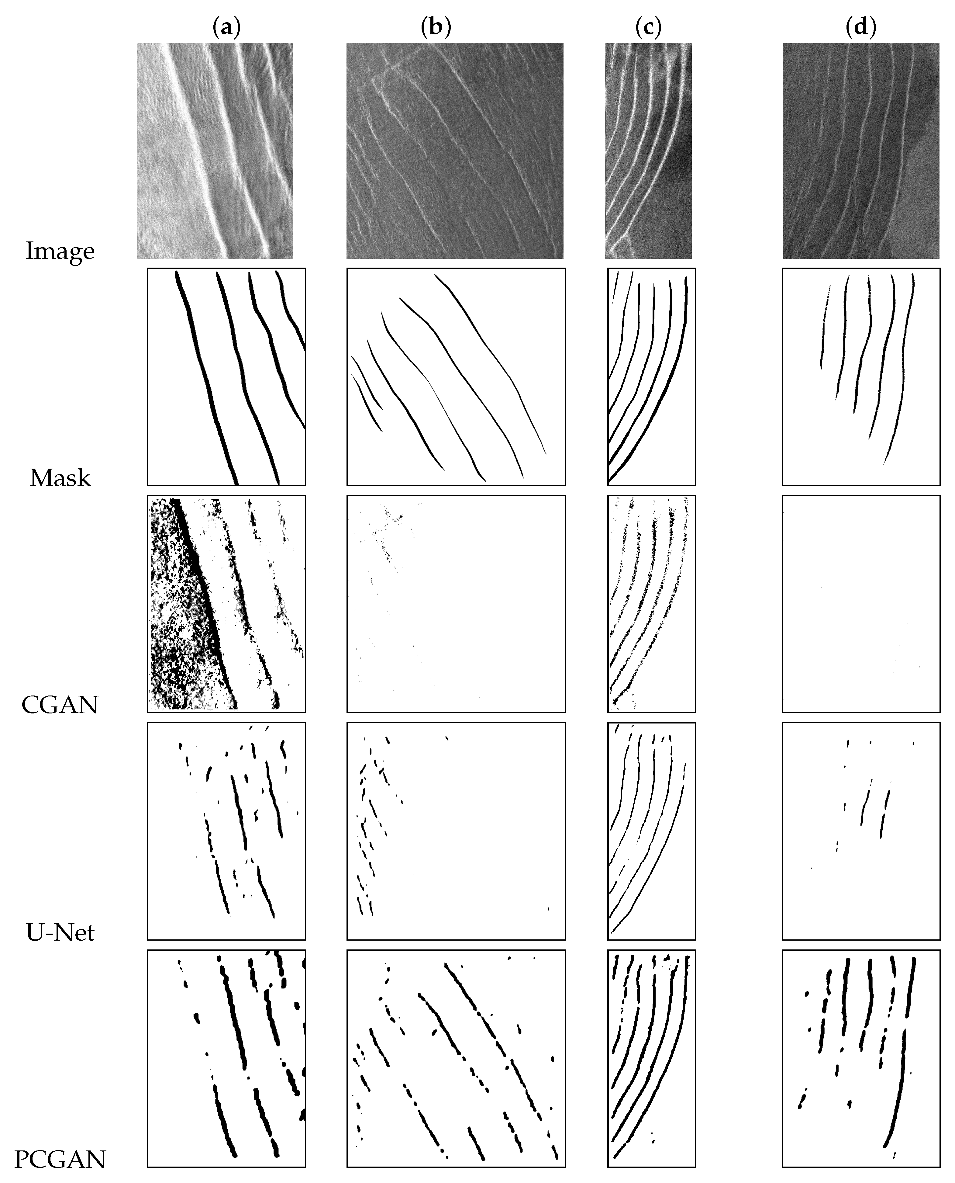
Figure 7 visually presents the detection outcomes for four distinct test scenarios, providing insights into the comparative performance of the detection models.
Figure 8 illustrates the recognition results of four internal wave images with different sizes, all from the Andaman Sea and featuring multiple wave crests within a single image.
Table 6 provides the average metrics across all test images of the same size and compares the performance of the five methods.
Table 7 presents the average metrics for an additional set of 40 images from the Andaman Sea and the South China Sea with varying sizes across three deep learning methods. In the table, the highest values for each metric are highlighted in cells with a gray background.
Figure 9 displays box plots illustrating the four evaluation metrics discussed in
Section 3.3 for the five detection methods. While our method may have a slightly lower maximum value compared to CGAN and U-Net, it outperforms other models in terms of both mean performance and stability.


