


Urban Green Connectivity Assessment: A Comparative Study of Datasets in European Cities
 ,
,  , ,
, ,  , , , and
Abstract
:1. Introduction
2. Material and Methods
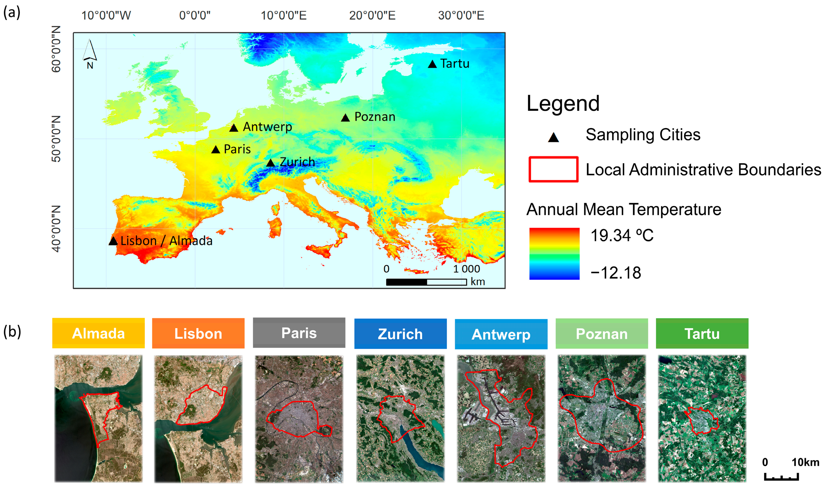
2.1. Study Area
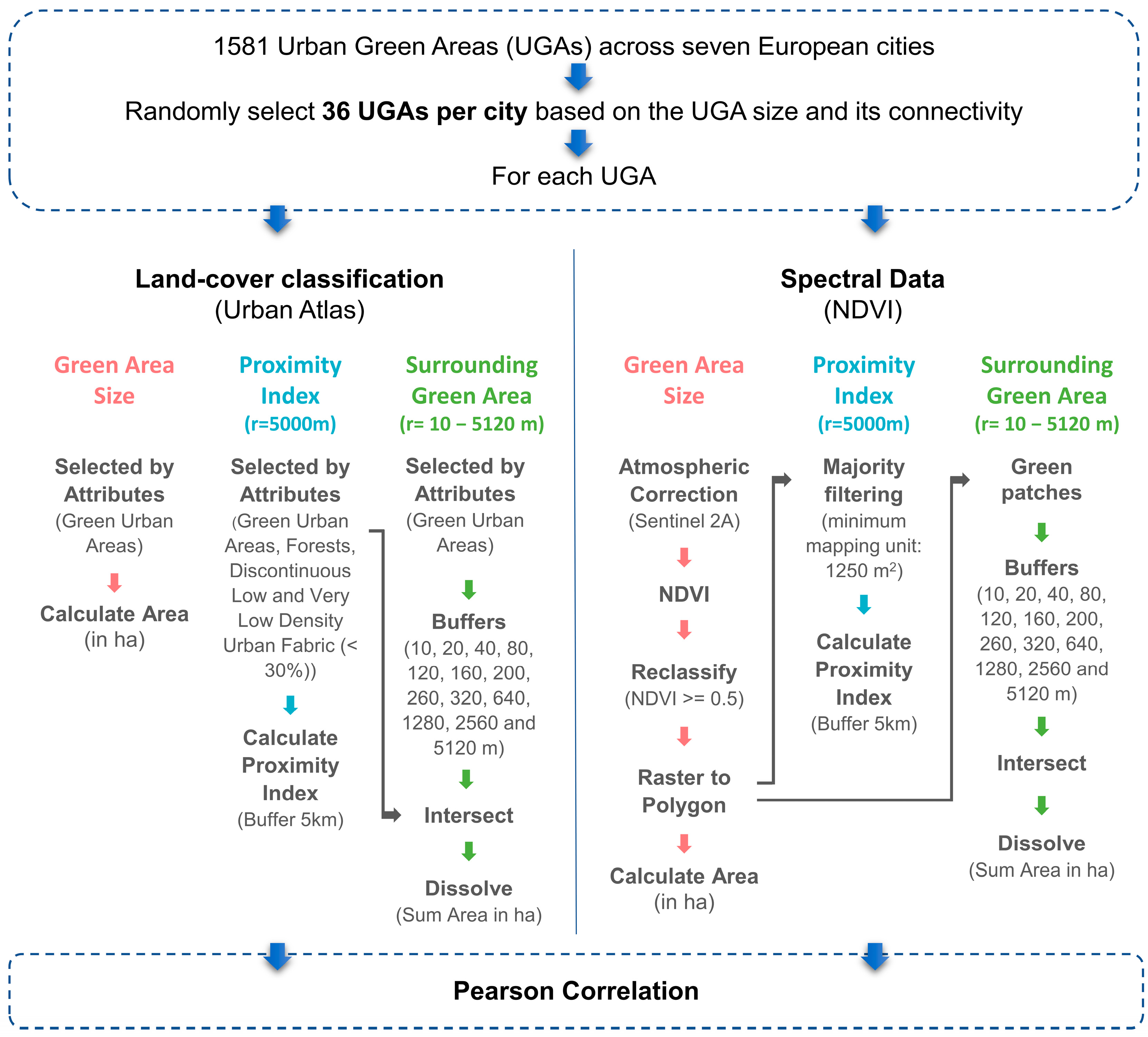
2.2. Data Collection
2.2.1. Land Cover Classification and Green Area Selection to Sample
2.2.2. Spectral Earth Observation Data
2.3. Landscape Metrics as Urban Green Connectivity Indicators
2.3.1. Green Area Size
2.3.2. Proximity Index
2.3.3. Amount of Surrounding Green Area at Multiple Distances
2.4. Data Analysis
3. Results
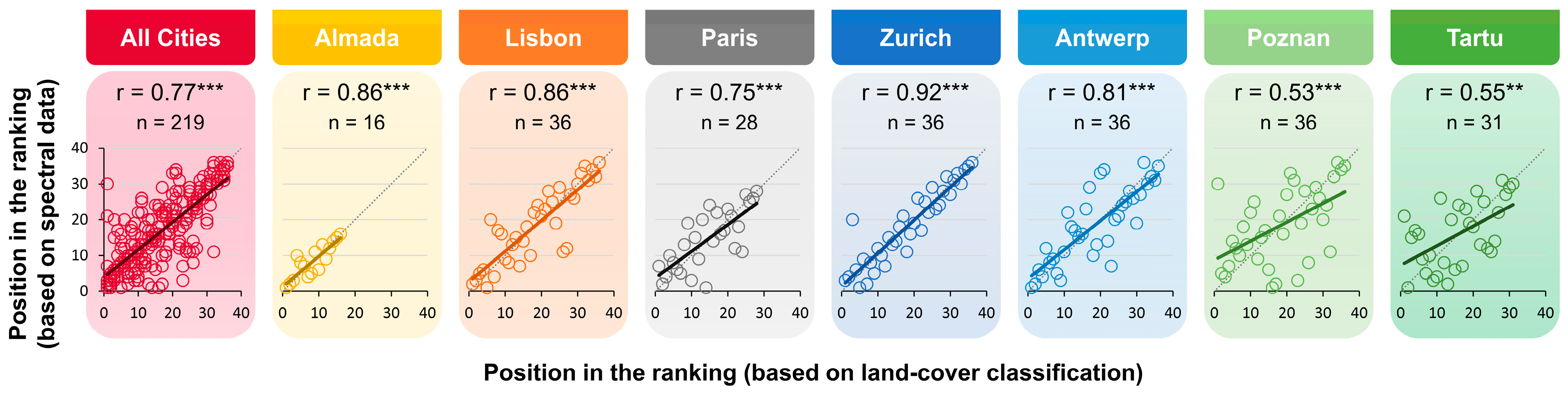
3.1. Green Area Size
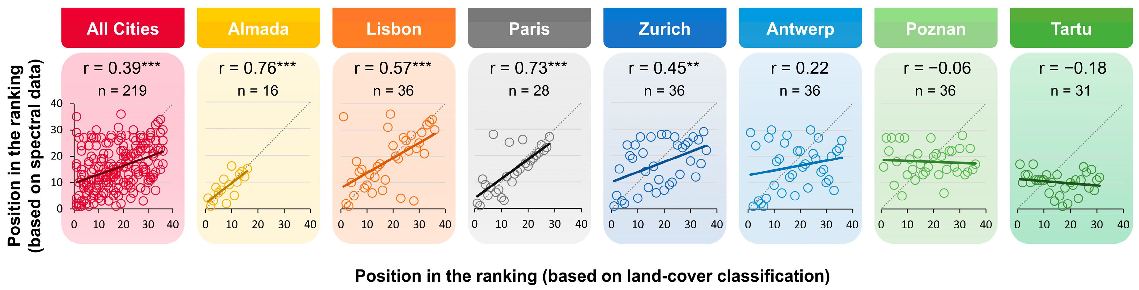
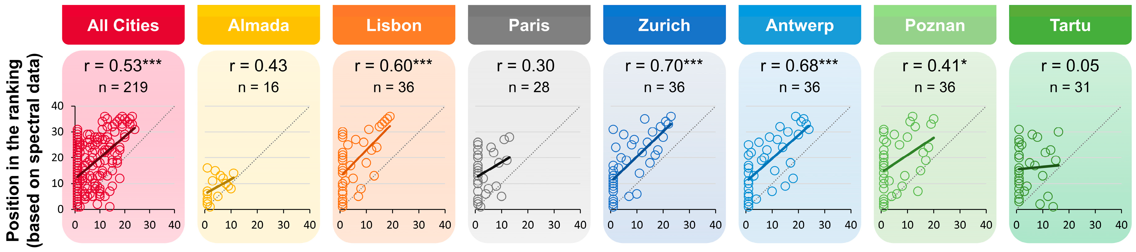
3.2. Proximity Index
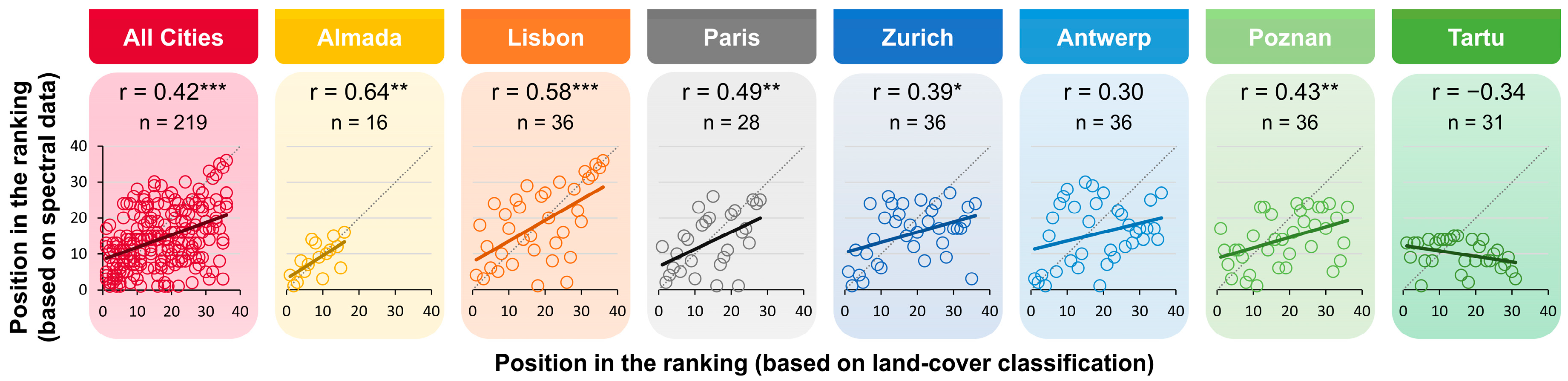
3.3. Number of Surrounding Green Areas at Multiple Distances
4. Discussion
4.1. Impact of Dataset Choice on Urban Green Connectivity Analysis
4.2. Factors Contributing to Disparities between Datasets
4.3. Advantages of Spectral Data in Urban Green Connectivity Analysis
4.4. Considerations for Land Cover Classification in Urban Green Connectivity Analysis
5. Conclusions
Supplementary Materials
Author Contributions
Funding
Data Availability Statement
Conflicts of Interest
References
- Chapman, C.; Hall, J.W. Designing green infrastructure and sustainable drainage systems in urban development to achieve multiple ecosystem benefits. Sustain. Cities Soc. 2022, 85, 104078. [Google Scholar] [CrossRef]
- United Nations. Department of Economic and Social Affairs, Population Division. World Urbanization Prospects: The 2018 Revision; United Nations: New York, NY, USA, 2019; Available online: https://www.un.org/development/desa/pd/sites/www.un.org.development.desa.pd/files/files/documents/2020/Jan/un_2018_wup_report.pdf (accessed on 17 May 2023).
- Colding, J. ‘Ecological land-use complementation’ for building resilience in urban ecosystems. Landsc. Urban Plan. 2007, 81, 46–55. [Google Scholar] [CrossRef]
- Houlden, V.; Jani, A.; Hong, A. Is biodiversity of greenspace important for human health and wellbeing? A bibliometric analysis and systematic literature review. Urban For. Urban Green. 2021, 66, 127385. [Google Scholar] [CrossRef]
- Lepczyk, C.A.; Aronson, M.F.J.; Evans, K.L.; Goddard, M.A.; Lerman, S.B.; MacIvor, J.S. Biodiversity in the City: Fundamental Questions for Understanding the Ecology of Urban Green Spaces for Biodiversity Conservation. BioScience 2017, 67, 799–807. [Google Scholar] [CrossRef]
- Casanelles-Abella, J.; Müller, S.; Keller, A.; Aleixo, C.; Orti, M.A.; Chiron, F.; Deguines, N.; Hallikma, T.; Laanisto, L.; Pinho, P.; et al. How wild bees find a way in European cities: Pollen metabarcoding unravels multiple feeding strategies and their effects on distribution patterns in four wild bee species. J. Appl. Ecol. 2021, 59, 457–470. [Google Scholar] [CrossRef]
- Threlfall, C.G.; Ossola, A.; Hahs, A.K.; Williams, N.S.G.; Wilson, L.; Livesley, S.J. Variation in Vegetation Structure and Composition across Urban Green Space Types. Front. Ecol. Evol. 2016, 4, 66. [Google Scholar] [CrossRef]
- Rösch, V.; Tscharntke, T.; Scherber, C.; Batáry, P. Biodiversity conservation across taxa and landscapes requires many small as well as single large habitat fragments. Oecologia 2015, 179, 209–222. [Google Scholar] [CrossRef] [PubMed]
- Barboza, E.P.; Cirach, M.; Khomenko, S.; Iungman, T.; Mueller, N.; Barrera-Gómez, J.; Rojas-Rueda, D.; Kondo, M.; Nieuwenhuijsen, M. Green space and mortality in European cities: A health impact assessment study. Lancet Planet. Health 2021, 5, e718–e730. [Google Scholar] [CrossRef]
- Fang, X.; Li, J.; Ma, Q. Integrating green infrastructure, ecosystem services and nature-based solutions for urban sustainability: A comprehensive literature review. Sustain. Cities Soc. 2023, 98, 104843. [Google Scholar] [CrossRef]
- Valente, D.; Marinelli, M.V.; Lovello, E.M.; Giannuzzi, C.G.; Petrosillo, I. Fostering the Resiliency of Urban Landscape through the Sustainable Spatial Planning of Green Spaces. Land 2022, 11, 367. [Google Scholar] [CrossRef]
- Gunawardena, K.R.; Wells, M.J.; Kershaw, T. Utilising green and bluespace to mitigate urban heat island intensity. Sci. Total Environ. 2017, 584–585, 1040–1055. [Google Scholar] [CrossRef]
- Ai, H.; Zhang, X.; Zhou, Z. The impact of greenspace on air pollution: Empirical evidence from China. Ecol. Indic. 2023, 146, 109881. [Google Scholar] [CrossRef]
- Massoni, E.S.; Barton, D.N.; Rusch, G.M.; Gundersen, V. Bigger, more diverse and better? Mapping structural diversity and its recreational value in urban green spaces. Ecosyst. Serv. 2018, 31, 502–516. [Google Scholar] [CrossRef]
- Lindemann-Matthies, P.; Brieger, H. Does urban gardening increase aesthetic quality of urban areas? A case study from Germany. Urban For. Urban Green. 2016, 17, 33–41. [Google Scholar] [CrossRef]
- Aronson, M.F.; Lepczyk, C.A.; Evans, K.L.; Goddard, M.A.; Lerman, S.B.; MacIvor, J.S.; Nilon, C.H.; Vargo, T. Biodiversity in the city: Key challenges for urban green space management. Front. Ecol. Environ. 2017, 15, 189–196. [Google Scholar] [CrossRef]
- Angold, P.; Sadler, J.; Hill, M.; Pullin, A.; Rushton, S.; Austin, K.; Small, E.; Wood, B.; Wadsworth, R.; Sanderson, R.; et al. Biodiversity in urban habitat patches. Sci. Total Environ. 2006, 360, 196–204. [Google Scholar] [CrossRef] [PubMed]
- Grafius, D.R.; Corstanje, R.; Harris, J.A. Linking ecosystem services, urban form and green space configuration using multivariate landscape metric analysis. Landsc. Ecol. 2018, 33, 557–573. [Google Scholar] [CrossRef] [PubMed]
- Nielsen, A.B.; Hedblom, M.; Olafsson, A.S.; Wiström, B. Spatial configurations of urban forest in different landscape and socio-political contexts: Identifying patterns for green infrastructure planning. Urban Ecosyst. 2016, 20, 379–392. [Google Scholar] [CrossRef]
- LaPoint, S.; Balkenhol, N.; Hale, J.; Sadler, J.; van der Ree, R. Ecological connectivity research in urban areas. Funct. Ecol. 2015, 29, 868–878. [Google Scholar] [CrossRef]
- Prastacos, P.; Lagarias, A.; Chrysoulakis, N. Using the Urban Atlas dataset for estimating spatial metrics. Methodology and application in urban areas of Greece. Cybergeo 2017, 815. [Google Scholar] [CrossRef]
- Buyantuyev, A.; Wu, J.; Gries, C. Multiscale analysis of the urbanization pattern of the Phoenix metropolitan landscape of USA: Time, space and thematic resolution. Landsc. Urban Plan. 2010, 94, 206–217. [Google Scholar] [CrossRef]
- Šímová, P.; Gdulová, K. Landscape indices behavior: A review of scale effects. Appl. Geogr. 2012, 34, 385–394. [Google Scholar] [CrossRef]
- Feltynowski, M.; Kronenberg, J.; Bergier, T.; Kabisch, N.; Łaszkiewicz, E.; Strohbach, M.W. Challenges of urban green space management in the face of using inadequate data. Urban For. Urban Green. 2018, 31, 56–66. [Google Scholar] [CrossRef]
- Badiu, D.L.; Iojă, C.I.; Pătroescu, M.; Breuste, J.; Artmann, M.; Niță, M.R.; Grădinaru, S.R.; Hossu, C.A.; Onose, D.A. Is urban green space per capita a valuable target to achieve cities’ sustainability goals? Romania as a case study. Ecol. Indic. 2016, 70, 53–66. [Google Scholar] [CrossRef]
- Biernacka, M.; Kronenberg, J.; Łaszkiewicz, E.; Czembrowski, P.; Parsa, V.A.; Sikorska, D. Beyond urban parks: Mapping informal green spaces in an urban–peri-urban gradient. Land Use Policy 2023, 131, 106746. [Google Scholar] [CrossRef]
- Wei, X.; Hu, M.; Wang, X.-J. The Differences and Influence Factors in Extracting Urban Green Space from Various Resolutions of Data: The Perspective of Blocks. Remote Sens. 2023, 15, 1261. [Google Scholar] [CrossRef]
- Buyantuyev, A.; Wu, J. Effects of thematic resolution on landscape pattern analysis. Landsc. Ecol. 2007, 22, 7–13. [Google Scholar] [CrossRef]
- Lin, Y.; An, W.; Gan, M.; Shahtahmassebi, A.; Ye, Z.; Huang, L.; Zhu, C.; Huang, L.; Zhang, J.; Wang, K. Spatial Grain Effects of Urban Green Space Cover Maps on Assessing Habitat Fragmentation and Connectivity. Land 2021, 10, 1065. [Google Scholar] [CrossRef]
- Saura, S. Effects of minimum mapping unit on land cover data spatial configuration and composition. Int. J. Remote Sens. 2010, 23, 4853–4880. [Google Scholar] [CrossRef]
- Wu, J. Effects of changing scale on landscape pattern analysis: Scaling relations. Landsc. Ecol. 2004, 19, 125–138. [Google Scholar] [CrossRef]
- Zhu, M.; Jiang, N.; Li, J.; Xu, J.; Fan, Y. The effects of sensor spatial resolution and changing grain size on fragmentation indices in urban landscape. Int. J. Remote Sens. 2007, 27, 4791–4805. [Google Scholar] [CrossRef]
- E.U. Mapping Guide for a European Urban Atlas v.4.7. 2006. Available online: https://land.copernicus.eu/user-corner/technical-library/urban-atlas-2012-mapping-guide-new (accessed on 25 January 2021).
- Muratet, A.; Lorrillière, R.; Clergeau, P.; Fontaine, C. Evaluation of landscape connectivity at community level using satellite-derived NDVI. Landsc. Ecol. 2012, 28, 95–105. [Google Scholar] [CrossRef]
- Wetherley, E.B.; Roberts, D.A.; McFadden, J.P. Mapping spectrally similar urban materials at sub-pixel scales. Remote Sens. Environ. 2017, 195, 170–183. [Google Scholar] [CrossRef]
- Wolff, M.; Haase, D.; Priess, J.; Hoffmann, T.L. The Role of Brownfields and Their Revitalisation for the Functional Connectivity of the Urban Tree System in a Regrowing City. Land 2023, 12, 333. [Google Scholar] [CrossRef]
- Casanelles-Abella, J.; Frey, D.; Muller, S.; Aleixo, C.; Alos Orti, M.; Deguines, N.; Hallikma, T.; Laanisto, L.; Niinemets, U.; Pinho, P.; et al. A dataset of the flowering plants (Angiospermae) in urban green areas in five European cities. Data Brief 2021, 37, 107243. [Google Scholar] [CrossRef] [PubMed]
- Muyshondt, B.; Wuyts, K.; Van Mensel, A.; Smets, W.; Lebeer, S.; Aleixo, C.; Ortí, M.A.; Casanelles-Abella, J.; Chiron, F.; Giacomo, P.; et al. Phyllosphere bacterial communities in urban green areas throughout Europe relate to urban intensity. FEMS Microbiol. Ecol. 2022, 98, fiac106. [Google Scholar] [CrossRef] [PubMed]
- Rocha, B.; Matos, P.; Giordani, P.; Piret, L.; Branquinho, C.; Casanelles-Abella, J.; Aleixo, C.; Deguines, N.; Hallikma, T.; Laanisto, L.; et al. Modelling the response of urban lichens to broad-scale changes in air pollution and climate. Environ. Pollut. 2022, 315, 120330. [Google Scholar] [CrossRef] [PubMed]
- Van Mensel, A.; Wuyts, K.; Pinho, P.; Muyshondt, B.; Aleixo, C.; Orti, M.A.; Casanelles-Abella, J.; Chiron, F.; Hallikma, T.; Laanisto, L.; et al. The magnetic signal from trunk bark of urban trees catches the variation in particulate matter exposure within and across six European cities. Environ. Sci. Pollut. Res. 2023, 30, 50883–50895. [Google Scholar] [CrossRef] [PubMed]
- Kopecká, M.; Szatmári, D.; Rosina, K. Analysis of Urban Green Spaces Based on Sentinel-2A: Case Studies from Slovakia. Land 2017, 6, 25. [Google Scholar] [CrossRef]
- McGarigal, K.; Marks, B.J. FRAGSTATS—Spatial Pattern Analysis Program for Quantifying Landscape Structure; Forest Science Department, Oregon State University: Corvallis, OR, USA, 1995. [Google Scholar] [CrossRef]
- Gustafson, E.J.; Parker, G.R. Relationships between landcover proportion and indices of landscape spatial pattern. Landsc. Ecol. 1992, 7, 101–110. [Google Scholar] [CrossRef]
- Lang, S.; Tiede, D. vLATE Extension für ArcGIS—Vektorbasiertes Tool zur quantitativen Landschaftsstrukturanalyse. In Proceedings of the ESRI European Conference for Users, Innsbruck, Austria, 8–10 October 2003; pp. 1–10. [Google Scholar]
- Lawler, J.J.; O’connor, R.J.; Hunsaker, C.T.; Jones, K.B.; Loveland, T.R.; White, D. The effects of habitat resolution on models of avian diversity and distributions: A comparison of two land-cover classifications. Landsc. Ecol. 2004, 19, 515–530. [Google Scholar] [CrossRef]
- Kabisch, N.; Strohbach, M.; Haase, D.; Kronenberg, J. Urban green space availability in European cities. Ecol. Indic. 2016, 70, 586–596. [Google Scholar] [CrossRef]
- Xu, F.; Yan, J.; Heremans, S.; Somers, B. Pan-European urban green space dynamics: A view from space between 1990 and 2015. Landsc. Urban Plan. 2022, 226, 104477. [Google Scholar] [CrossRef]
- Fuller, R.A.; Gaston, K.J. The scaling of green space coverage in European cities. Biol. Lett. 2009, 5, 352–355. [Google Scholar] [CrossRef] [PubMed]
- Wellmann, T.; Haase, D.; Knapp, S.; Salbach, C.; Selsam, P.; Lausch, A. Urban land use intensity assessment: The potential of spatio-temporal spectral traits with remote sensing. Ecol. Indic. 2018, 85, 190–203. [Google Scholar] [CrossRef]
- Jelinski, D.E.; Wu, J. The modifiable areal unit problem and implications for landscape ecology. Landsc. Ecol. 1996, 11, 129–140. [Google Scholar] [CrossRef]
- Hay, G.; Marceau, D.; Dubé, P.; Bouchard, A. A multiscale framework for landscape analysis: Object-specific analysis and upscaling. Landsc. Ecol. 2001, 16, 471–490. [Google Scholar] [CrossRef]
- Cash, D.W.; Adger, W.N.; Berkes, F.; Garden, P.; Lebel, L.; Olsson, P.; Pritchard, L.; Young, O. Scale and cross-scale dynamics: Governance and information in a multilevel world. Ecol. Soc. 2006, 11, 12. Available online: https://www.jstor.org/stable/26265993 (accessed on 14 September 2023). [CrossRef]
- Wang, W.; Jiao, L.; Jia, Q.; Liu, J.; Mao, W.; Xu, Z.; Li, W. Land use optimization modelling with ecological priority perspective for large-scale spatial planning. Sustain. Cities Soc. 2020, 65, 102575. [Google Scholar] [CrossRef]
- Zięba-Kulawik, K.; Wężyk, P. Monitoring 3D Changes in Urban Forests Using Landscape Metrics Analyses Based on Multi-Temporal Remote Sensing Data. Land 2022, 11, 883. [Google Scholar] [CrossRef]


| City | City Area (ha) | Pop. Density (hab.km2) | Green Area (ha and %) | No. of UGAs | Climate | Temperature (°C) | Precipitation (mm) | Aridity Index |
|---|---|---|---|---|---|---|---|---|
| Almada | 6999 | 3728 | 1580 (23%) | 130 | Mediterranean | 16.2 | 685 | 0.71 |
| Antwerp | 22,416 | 2438 | 2436 (11%) | 111 | Temperate maritime | 10.5 | 796 | 1.09 |
| Lisbon | 8687 | 6429 | 1393 (16%) | 170 | Mediterranean | 16.7 | 712 | 0.73 |
| Paris | 10,492 | 20,238 | 1706 (16%) | 420 | Temperate | 11.9 | 649 | 0.77 |
| Poznan | 25,628 | 2088 | 4869 (19%) | 425 | Temperate continental | 8.6 | 505 | 0.70 |
| Tartu | 3882 | 2240 | 479 (12%) | 128 | Hemi-boreal | 5.5 | 617 | 1.03 |
| Zurich | 9200 | 4867 | 2774 (30%) | 197 | Temperate, mild | 9.5 | 1115 | 1.48 |
| Selected Classes | Minimum Mapping Unit | Criteria | |
|---|---|---|---|
| Selected urban atlas classes | Green urban areas a,b | 0.25 ha | Classes with at least 70% of the total class area covered by vegetation and a high probability of having trees. |
| Forests b | 1 ha | ||
| Discontinuous very low-density urban fabric (soil sealing level (S.L.) < 10%) b | 0.25 ha | ||
| Discontinuous low-density urban fabric (S.L. 10–30%) b | 0.25 ha | ||
| NDVI threshold | NDVI ≥ 0.5 | 0.01 ha or 0.125 ha, depending on the estimated landscape metric | Class characterized by UGAs with high vegetative vigor, including trees and irrigated/fertilized lawns. This class is functionally important throughout the year and has a homogeneous land-use intensity. |
| Almada | Antwerp | Lisbon | Paris | Poznan | Tartu | Zurich | ||
|---|---|---|---|---|---|---|---|---|
| Number of patches | 16 | 36 | 36 | 28 | 36 | 31 | 36 | |
| Total patch area (ha) | 100.04 | 334.39 | 181.56 | 693.24 | 252.37 | 165.04 | 130.70 | |
| Total connectivity | 25,103.36 | 13,026.80 | 43,339.28 | 51,271.32 | 23,718.58 | 2746.40 | 38,282.03 | |
| Patch size (ha) | Max | 43.56 | 108.59 | 30.85 | 588.09 | 103.34 | 30.79 | 27.45 |
| Min | 0.30 | 0.38 | 0.33 | 0.26 | 0.26 | 0.31 | 0.27 | |
| Average | 6.25 | 9.29 | 5.04 | 24.76 | 7.01 | 5.32 | 3.63 | |
| Median | 1.89 | 2.66 | 2.62 | 1.01 | 2.34 | 1.76 | 1.88 | |
| Standard deviation | 10.70 | 24.03 | 6.86 | 110.53 | 17.96 | 7.55 | 5.20 | |
| Patch connectivity | Max | 23,807.54 | 3995.62 | 12,202.27 | 45,794.28 | 12,829.47 | 624.85 | 26,935.38 |
| Min | 1.30 | 1.52 | 0.64 | 1.77 | 2.16 | 1.95 | 4.87 | |
| Average | 1568.96 | 361.86 | 1203.87 | 1831.12 | 658.85 | 88.59 | 1063.39 | |
| Median | 10.99 | 53.03 | 22.72 | 6.94 | 16.40 | 14.97 | 42.60 | |
| Standard deviation | 5931.57 | 828.97 | 3132.94 | 8634.21 | 2168.17 | 161.03 | 4504.75 | |
Disclaimer/Publisher’s Note: The statements, opinions and data contained in all publications are solely those of the individual author(s) and contributor(s) and not of MDPI and/or the editor(s). MDPI and/or the editor(s) disclaim responsibility for any injury to people or property resulting from any ideas, methods, instructions or products referred to in the content. |
© 2024 by the authors. Licensee MDPI, Basel, Switzerland. This article is an open access article distributed under the terms and conditions of the Creative Commons Attribution (CC BY) license (https://creativecommons.org/licenses/by/4.0/).
Share and Cite
Aleixo, C.; Branquinho, C.; Laanisto, L.; Tryjanowski, P.; Niinemets, Ü.; Moretti, M.; Samson, R.; Pinho, P. Urban Green Connectivity Assessment: A Comparative Study of Datasets in European Cities. Remote Sens. 2024, 16, 771. https://doi.org/10.3390/rs16050771
Aleixo C, Branquinho C, Laanisto L, Tryjanowski P, Niinemets Ü, Moretti M, Samson R, Pinho P. Urban Green Connectivity Assessment: A Comparative Study of Datasets in European Cities. Remote Sensing. 2024; 16(5):771. https://doi.org/10.3390/rs16050771
Chicago/Turabian StyleAleixo, Cristiana, Cristina Branquinho, Lauri Laanisto, Piotr Tryjanowski, Ülo Niinemets, Marco Moretti, Roeland Samson, and Pedro Pinho. 2024. "Urban Green Connectivity Assessment: A Comparative Study of Datasets in European Cities" Remote Sensing 16, no. 5: 771. https://doi.org/10.3390/rs16050771