Power-Type Structural Self-Constrained Inversion Methods of Gravity and Magnetic Data

Abstract

The inversion of gravity and magnetic data can obtain the density and magnetic structure of underground space, which provide important information for resource exploration and geological structure division. The most commonly used inversion method is smooth inversion in which the objective function is built with L2-norm, which has good stability, but it produces non-focused results that make subsequent interpretation difficult. The power-type structural self-constrained inversion (PTSS) method with L2-norm is proposed to improve the resolution of smooth inversion. A self-constraint term based on the power gradient of the results is introduced, which takes advantage of the structural feature that the power gradient can better focus on the model boundary to improve the resolution. For the joint inversion of gravity and magnetic data, the power-type mutual-constrained term between different physical structures and the self-constrained term can be simultaneously used to obtain higher-resolution results. The modeling tests demonstrated that the PTSS method can produce converged high-resolution results with good noise immunity in both the respective inversions and the joint inversion. Then, the PTSS joint inversion was applied to the airborne gravity and magnetic data of the iron ore district in Shandong, revealing the shape and location of the mineralized rock mass, which are crucial information for subsequent detailed exploration.

1. Introduction

Gravity and magnetic methods, as a common means of remote sensing measurements, are widely used in oil, gas, and mineral surveys, the interpretation of geological formations, and environmental and engineering investigations [1,2,3,4]. The inversions of gravity and magnetic data are important methods for obtaining three-dimensional density and magnetic susceptibility (or magnetization) distributions. Gravity and magnetic data inversion is an ill-posed problem, which means that there exists an infinite number of models that can reasonably fit the data. Tikhonov and Arsenin effectively reduced the non-unique problem of inversion by introducing a regularization stabilizer [5]. In this method, the objective function of the inversion consists of a fitting error function and a regularization stabilizer.

A general method in gravity and magnetic inversion is the smooth inversion method, which incorporates a smooth stabilizer built with L2-norm [6,7]. The smooth inversion method is highly stable and universal, but its results of inversions are usually ambiguous and non-focused. Therefore, the low resolution of the smoothed inversion method increases the difficulty of subsequent interpretation, especially in mineral exploration. [8,9]. Therefore, the proposal of high-resolution gravity and magnetic inversion methods is an important research direction.

In one such approach, researchers proposed the non-smooth stabilizer to replace the general smooth stabilizer and identified the physical bounds from a priori information to obtain results with sharp boundaries, such as the minimum support stabilizer, known as the L₀-norm stabilizer [10], the minimum gradient support stabilizer [11], the L₁-norm stabilizer [8], the Cauchy norm stabilizer [12], the zero-order minimum entropy stabilizer [13], the sigmoid stabilizing function [14], and the error function stabilizer [15]. Another approach to improve the inversion resolution of gravity and magnetic data is the joint inversion of multiple geophysical data. Depending on whether the physical models corresponding to different observations are the same and relevant, there are two groups of joint inversion. The first group is the joint inversion of different geophysical data corresponding to the same physical model, such as gravity and gravity gradient data joint inversion for density structure [16,17,18,19,20]. It can recover high-resolution models at different depths by exploiting the fact that the gradient data are more sensitive to shallow sources, and field data emphasize the response of deep sources. The second group is the joint inversion of different kinds of geophysical data corresponding to different physical property models. For this type of joint inversion, correlations between different petrophysical parameters or geometries are established to facilitate complementary interactions among diverse geophysical methods, such as cross-gradient joint inversion methods [21,22,23,24,25,26], correlation-constrained methods [27,28,29], Gramian-constrained joint inversion methods [30,31,32,33], and joint inversion based on deep learning [34,35,36]. In addition, several researchers have incorporated geologic information into the inversion of gravity and magnetic data to produce models with higher resolution. Rock physical information can be incorporated into the objective function of the inversion as a reference model or equation constraint to improve the resolution of the inversion results [37,38,39,40,41]. In addition, the inversion results can be improved by adding tectonic direction information extracted from geologic maps and seismic imaging [42,43,44]. However, these methods often rely heavily on prior geological information and a variety of geophysical data available.

In this paper, power-type structural self-constrained inversion (PTSS) methods are proposed to improve resolution in smooth inversion. A self-constraint term is introduced, which is constructed using the gradient power of the initial result in the smoothing inversion. This term enhances the strength of the constraints at the boundary locations of the model and suppresses the strength of the constraints at other locations, making the inversion more convergent. In the joint inversion, the power-type structural mutual-constrained term is constructed to enhance mutual constraints between different physical structures; in addition, the self-constrained term can be incorporated into the inversion process to further improve the resolution and maintain their respective structural features. The novel approach has been tested by synthetic examples and airborne gravity and magnetic data collected over the iron ore district in Shandong. The inversion results demonstrated the ability and efficiency of the smooth inversion method with power-type structural self-constrained term to recover geologic models with high resolution.

2. Methodology

2.1. Forward and Inversion Method

In forward modeling, the exploration space needs to be subdivided into a number of subdivided cells. The gravity and magnetic anomaly response induced by each cell can be calculated by the formula given by Blakely [45], and the matrix form of the formula for the forward modeling can be written as

$$\mathit{d}=\mathit{A}\mathit{m},$$

(1)

where d is the gravity or magnetic anomaly data; m is the physical parameter (density ρ or magnetization M) of all subdivided cells; and A is the matrix of forward kernel functions representing the gravity or magnetic anomaly response of each cell to all observed point locations. The inversion of gravity and magnetic data is a process of solving the physical property parameters with known observed anomalies and kernel function matrix. Since gravitational and magnetic anomaly inversion is an ill-posed problem, there exists an infinite number of models that can fit the observed anomalies. Tikhonov and Arsenin effectively reduced the non-uniqueness of the inversion by introducing a regularization stabilizer [5]. The objective function can be expressed as

$$\varphi ={\varphi }_d+\alpha {\varphi }_m,$$

(2)

Here, $\varphi$ depicts the data misfit function as follows:

$${\varphi }_d={‖\mathit{A}\mathit{m}-\mathit{d}‖}_2^2,$$

(3)

where $\alpha$ is the regularization factor that is actually determined by the L-curve method, which has the role of determining the misfit weight and the corresponding weight of the stabilizer ${\varphi }_m$ in the Tikhonov parametric functional [46]. In the inversion of gravity and magnetic data, the stabilizer ${\varphi }_m$ could be formulated analogously to a pseudo-quadratic function such that

$${\varphi }_m={‖{\mathit{W}}_d{\mathit{W}}_m\mathit{m}‖}_2^2,$$

(4)

where W_d is a depth-weighting operator, which gives different weights to each cell based on its depth, and it is used to counteract the decay of the kernel function with depth. The depth weight operator is expressed as

$${\mathit{W}}_d=diag\left[z^{-\beta /2}\right],$$

(5)

Here, z is the depth of the subdivision cell. Because of the different decay rates of the gravity and magnetic forward kernel functions, β is usually 2 in gravity data inversion and 3 in magnetic data inversion. W_m is the model weighting operator when it is unit matrix, ϕ is the objective function of smooth inversion, and ϕ_m is the L2-norm stabilizer.

The conjugate gradient method can be used to solve the inverse problem in Equation (2) and terminate the iteration when the mean fitting error is less than the maximum anomaly multiplied by 10⁻⁷. Finally, the physical distribution of the exploration space is obtained.

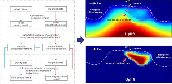
2.2. Power-Type Structural Self-Constrained (PTSS) Inversion Method

In joint inversion, structural constraints are established by different physical structures to facilitate complementary interactions among diverse geophysical methods, thereby obtaining high-resolution models. The structurally constrained joint inversion objective function of gravity and magnetic data can be written as

$$\varphi \left(\mathit{\rho },\mathit{M}\right)=\left[\begin{array}{c}{\varphi }_{gra}\\ {\varphi }_{mag}\end{array}\right]+\left[\begin{array}{c}{\alpha }_{\mathit{\rho }}{\varphi }_{\mathit{\rho }}\\ {\alpha }_M{\varphi }_M\end{array}\right]+\left[\begin{array}{c}{\lambda }_{\mathit{\rho }}{\varphi }_{s,\mathit{\rho }}\\ {\lambda }_M{\varphi }_{s,M}\end{array}\right],$$

(6)

where ϕ_gra and ϕ_ρ are the data misfit term and stabilizer for the gravity part of joint inversion, and ϕ_mag and ϕ_M are for the magnetic inversion. ϕ_s,ρ and ϕ_s,M are the structurally constrained terms for gravity and magnetic inversion, such as cross-gradient function [21]. α_ρ and α_M are the regularization parameters for gravity and magnetic inversion. λ_ρ and λ_M are the weighting factors for structural constraints. In the cross-gradient joint inversion of the gravity and magnetic data, the density structure is used to constrain the magnetic inversion, and the magnetic susceptibility structure is used to constrain the gravity inversion.

The structural self-constrained strategies are proposed (Figure 1) for the respective inversions and the joint inversion based on the ideology of structural constraints to obtain high-resolution results.

In the respective inversion, a self-constraint term is formed based on the initial result and introduced into subsequent inversion. The objective function of the self-constrained inversion is given by

$$\varphi ={\varphi }_d+\alpha {\varphi }_m+\lambda {\varphi }_{self},$$

(7)

where ${\varphi }_{self}$ is the self-constraint. λ are the weighting factors for the structural self-constrained term, and its magnitude is related to the order of magnitude of the kernel function and the physical property gradient, which are usually taken as 10¹⁰~10¹². Considering that the physical gradient is smooth since the smooth inversion results in divergence, the self-constrained term constructed by the smooth physical gradients is not sufficient to produce more focused results. Therefore, the self-constraint term is built with physical gradient power, and the term utilizes the feature that the physical gradient power focuses on the model boundary to make the subsequent inversion results converge to the boundary, thus improving the inversion resolution. The gravity data inversion is used as an example to construct the power-type structural self-constrained term as Equation (8).

$${\varphi }_{self}={‖\overrightarrow{\mathit{t}}‖}_2^2={‖{\left(\nabla {\mathit{\rho }}_{inv}\right)}^n\times \nabla \mathit{\rho }‖}_2^2,$$

(8)

where $\overrightarrow{\mathit{t}}$ represents the cross-gradient vector of initial density results ρ_inv and unknown density ρ, and $\nabla$ is the gradient operator, n is the index of $\nabla {\mathit{\rho }}_{inv}$. t_x, t_y, and t_z are the components of $\overrightarrow{\mathit{t}}$ in the x, y, and z directions, respectively, and their expansion is given by

$$\overrightarrow{\mathit{t}}={\left(\nabla {\mathit{\rho }}_{inv}\right)}^n\times \nabla \mathit{\rho }=\left({\mathit{t}}_x,{\mathit{t}}_y,{\mathit{t}}_z\right),$$

(9)

$${\mathit{t}}_x={\left(\nabla {\mathit{\rho }}_{inv}\right)}_y^n{\mathit{\rho }}_{\mathrm{z}}-{\left(\nabla {\mathit{\rho }}_{inv}\right)}_z^n{\mathit{\rho }}_y$$

(10)

$${\mathit{t}}_y={\left(\nabla {\mathit{\rho }}_{inv}\right)}_z^n{\mathit{\rho }}_x-{\left(\nabla {\mathit{\rho }}_{inv}\right)}_x^n{\mathit{\rho }}_z$$

(11)

$${\mathit{t}}_z={\left(\nabla {\mathit{\rho }}_{inv}\right)}_x^n{\mathit{\rho }}_y-{\left(\nabla {\mathit{\rho }}_{inv}\right)}_y^n{\mathit{\rho }}_x$$

(12)

Here, (${\mathit{\rho }}_x$, ${\mathit{\rho }}_y$, ${\mathit{\rho }}_z$) and [${\left(\nabla {\mathit{\rho }}_{inv}\right)}_x^n$, ${\left(\nabla {\mathit{\rho }}_{inv}\right)}_y^n$, ${\left(\nabla {\mathit{\rho }}_{inv}\right)}_z^n$] are the gradients of $\mathit{\rho }$ and ${\left(\nabla {\mathit{\rho }}_{inv}\right)}^n$ in the x, y, and z directions. For the physical gradients (${\mathit{\rho }}_x$, ${\mathit{\rho }}_y$, ${\mathit{\rho }}_z$), the center difference calculation is used to simplify the gradient calculation as

$${\mathit{\rho }}_x={\mathit{D}}_x\mathit{\rho },$$

(13)

$${\mathit{\rho }}_y={\mathit{D}}_y\mathit{\rho }$$

(14)

$${\mathit{\rho }}_z={\mathit{D}}_z\mathit{\rho }$$

(15)

For [${\left(\nabla {\mathit{\rho }}_{inv}\right)}_x^n$, ${\left(\nabla {\mathit{\rho }}_{inv}\right)}_y^n$, ${\left(\nabla {\mathit{\rho }}_{inv}\right)}_z^n$], the modulus of the physical total gradient $\left|\nabla {\mathit{\rho }}_{inv}\right|$ and the declination i and inclination δ of the physical gradient need to be calculated first. They can be written separately as

$$\left|\nabla {\mathit{\rho }}_{inv}\right|=\sqrt{{{\mathit{\rho }}_{x,inv}}^2+{{\mathit{\rho }}_{y,inv}}^2+{{\mathit{\rho }}_{z,inv}}^2}$$

(16)

$$\mathit{i}=\arcsin \left({\mathit{\rho }}_{z,inv}/\left|\nabla {\mathit{\rho }}_{inv}\right|\right)$$

(17)

$$\mathit{\delta }=\arctan \left({\mathit{\rho }}_{x,inv}/{\mathit{\rho }}_{y,inv}\right)$$

(18)

Next, the nth powers of $\left|\nabla {\mathit{\rho }}_{inv}\right|$ and [${\left(\nabla {\mathit{\rho }}_{inv}\right)}_x^n$, ${\left(\nabla {\mathit{\rho }}_{inv}\right)}_y^n$, ${\left(\nabla {\mathit{\rho }}_{inv}\right)}_z^n$] in Equations (9)–(12) can be rewritten based on Equations (16)–(18) as

$${\left|\nabla {\mathit{\rho }}_{inv}\right|}^n={\left(\sqrt{{{\mathit{\rho }}_{x,inv}}^2+{{\mathit{\rho }}_{y,inv}}^2+{{\mathit{\rho }}_{z,inv}}^2}\right)}^n$$

(19)

$${\left(\nabla {\mathit{\rho }}_{inv}\right)}_x^n=\frac{{\mathit{\rho }}_{x,inv}}{\left|{\mathit{\rho }}_{x,inv}+e\right|}\cdot \left|\cos \mathit{\delta }\cos \mathit{i}{\left|\nabla {\mathit{\rho }}_{inv}\right|}^n\right|$$

(20)

$${\left(\nabla {\mathit{\rho }}_{inv}\right)}_y^n=\frac{{\mathit{\rho }}_{y,inv}}{\left|{\mathit{\rho }}_{y,inv}+e\right|}\cdot \left|\cos \mathit{\delta }\sin \mathit{i}{\left|\nabla {\mathit{\rho }}_{inv}\right|}^n\right|$$

(21)

$${\left(\nabla {\mathit{\rho }}_{inv}\right)}_z^n=\frac{{\mathit{\kappa }}_x}{\left|{\mathit{\rho }}_{y,inv}+e\right|}\cdot \left|\sin \mathit{i}{\left|\nabla {\mathit{\rho }}_{inv}\right|}^n\right|$$

(22)

where e is a constant which is infinitely close to zero, and it is used to eliminate the singularity. Using Equations (9)–(22), the self-constraint term can be rewritten as

$$\begin{array}{ll}{\varphi }_{self}& ={‖\overrightarrow{\mathit{t}}‖}_2^2={‖{\left(\nabla {\mathit{\rho }}_{inv}\right)}^n\times \nabla \mathit{\rho }‖}_2^2={‖{\overrightarrow{\mathit{t}}}_x‖}_2^2+{‖{\overrightarrow{\mathit{t}}}_y‖}_2^2+{‖{\overrightarrow{\mathit{t}}}_z‖}_2^2\\ & ={‖{\mathit{B}}_x\mathit{\rho }‖}_2^2+{‖{\mathit{B}}_y\mathit{\rho }‖}_2^2+{‖{\mathit{B}}_z\mathit{\rho }‖}_2^2\end{array},$$

(23)

$${\mathit{B}}_x={\left(\nabla {\mathit{\rho }}_{inv}\right)}_y^n{\mathit{D}}_z-{\left(\nabla {\mathit{\rho }}_{inv}\right)}_z^n{\mathit{D}}_y$$

(24)

$${\mathit{B}}_y={\left(\nabla {\mathit{\rho }}_{inv}\right)}_z^n{\mathit{D}}_x-{\left(\nabla {\mathit{\rho }}_{inv}\right)}_x^n{\mathit{D}}_z$$

(25)

$${\mathit{B}}_z={\left(\nabla {\mathit{\rho }}_{inv}\right)}_x^n{\mathit{D}}_y-{\left(\nabla {\mathit{\rho }}_{inv}\right)}_y^n{\mathit{D}}_x$$

(26)

From Equations (23)–(26), the physical meaning of the structural self-constraints is to make the gradient of the solved density ρ as consistent as possible with the gradient of the initial model ρ_inv during the solution process ($\overrightarrow{\mathit{t}}$ is 0 when ρ and ρ_inv are identical). As n increases, the inversion results will be more focused on the model boundaries which are the locations of high values of the gradient.

Rocks with different lithologies have different densities and magnetic properties, so the density and magnetic structure are usually similar. Magnetic data have a higher horizontal resolution, and it highlights shallow source response but suppresses deep source response, while gravity data can better recover the structural characteristics of deep field sources. Therefore, the joint inversion of gravity and magnetic data can enhance accuracy by establishing mutual constraints between density and magnetic structure.

In joint inversion, power-type structural mutual constrained term ${\varphi }_{mut}$ is given to enhance mutual constraints between different physical structures. Regarding gravity data in joint inversion, the term ${\varphi }_{mut,\rho }$ can be written as

$$\begin{array}{ll}{\varphi }_{mut,\rho }& ={‖{\overrightarrow{\mathit{t}}}_{gra}‖}_2^2={‖{\left(\nabla {\mathit{M}}_{inv}\right)}^n\times \nabla \mathit{\rho }‖}_2^2\\ & ={‖{\mathit{B}}_{M,x}\mathit{\rho }‖}_2^2+{‖{\mathit{B}}_{M,y}\mathit{\rho }‖}_2^2+{‖{\mathit{B}}_{M,z}\mathit{\rho }‖}_2^2\end{array},$$

(27)

$${\mathit{B}}_{M,x}={\left(\nabla {\mathit{M}}_{inv}\right)}_y^n{\mathit{D}}_z-{\left(\nabla {\mathit{M}}_{inv}\right)}_z^n{\mathit{D}}_y$$

(28)

$${\mathit{B}}_{M,y}={\left(\nabla {\mathit{M}}_{inv}\right)}_z^n{\mathit{D}}_x-{\left(\nabla {\mathit{M}}_{inv}\right)}_x^n{\mathit{D}}_z$$

(29)

$${\mathit{B}}_{M,z}={\left(\nabla {\mathit{M}}_{inv}\right)}_x^n{\mathit{D}}_y-{\left(\nabla {\mathit{M}}_{inv}\right)}_y^n{\mathit{D}}_x$$

(30)

and the term for magnetic data inversion ${\varphi }_{mut,M}$ can be written as

$$\begin{array}{ll}{\varphi }_{mut,M}& ={‖{\overrightarrow{\mathit{t}}}_{mag}‖}_2^2={‖{\left(\nabla {\mathit{\rho }}_{inv}\right)}^n\times \nabla \mathit{M}‖}_2^2\\ & ={‖{\mathit{B}}_{\mathit{\rho },x}\mathit{M}‖}_2^2+{‖{\mathit{B}}_{\mathit{\rho },y}\mathit{M}‖}_2^2+{‖{\mathit{B}}_{\mathit{\rho },z}\mathit{M}‖}_2^2\end{array}.$$

(31)

$${\mathit{B}}_{\mathit{\rho },x}={\left(\nabla {\mathit{\rho }}_{inv}\right)}_y^n{\mathit{D}}_z-{\left(\nabla {\mathit{\rho }}_{inv}\right)}_z^n{\mathit{D}}_y$$

(32)

$${\mathit{B}}_{\mathit{\rho },y}={\left(\nabla {\mathit{\rho }}_{inv}\right)}_z^n{\mathit{D}}_x-{\left(\nabla {\mathit{\rho }}_{inv}\right)}_x^n{\mathit{D}}_z$$

(33)

$${\mathit{B}}_{\mathit{\rho },z}={\left(\nabla {\mathit{\rho }}_{inv}\right)}_x^n{\mathit{D}}_y-{\left(\nabla {\mathit{\rho }}_{inv}\right)}_y^n{\mathit{D}}_x$$

(34)

The introduction of the mutual constraint term ${\varphi }_{mut}$ into the inversion makes the density inversion results $\mathit{\rho }$ similar to the initial magnetic inversion results ${\mathit{M}}_{inv}$, giving them higher horizontal resolution and improving the recovery of shallow field sources. The magnetic inversion results $\mathit{M}$ are similar to the initial density results ${\mathit{\rho }}_{inv}$, which enable better recovery of the magnetic structure of the deep field sources.

On this basis, the self-constrained term is introduced into the objective function of the joint inversion to further enhance the resolution and maintain the structural features of the respective inversion results. The objective function of the power-type structural constrained joint inversion is written as

$$\varphi \left(\mathit{\rho },\mathit{M}\right)=\left[\begin{array}{c}{\varphi }_{gra}\\ {\varphi }_{mag}\end{array}\right]+\left[\begin{array}{c}{\alpha }_{\mathit{\rho }}{\varphi }_{\mathit{\rho }}\\ {\alpha }_M{\varphi }_M\end{array}\right]+\left[\begin{array}{c}{\lambda }_{self,\mathit{\rho }}{\varphi }_{self,\mathit{\rho }}\\ {\lambda }_{self,M}{\varphi }_{self,M}\end{array}\right]+\left[\begin{array}{c}{\lambda }_{mut,\mathit{\rho }}{\varphi }_{mut,\mathit{\rho }}\\ {\lambda }_{mut,M}{\varphi }_{mut,M}\end{array}\right].$$

(35)

where ${\varphi }_{self,\rho }$ and ${\varphi }_{self,M}$ are self-constrained terms for gravity and magnetic inversion in joint inversion. (${\lambda }_{self,\rho }$, ${\lambda }_{self,M}$) and (${\lambda }_{mut,\rho }$, ${\lambda }_{mut,M}$) are the weights factors for structural self-constrained term and mutual-constrained term to adjust the constraint strength, and they are taken as 10¹²⁻²ⁿ for gravity inversion and 10¹⁰⁻²ⁿ for magnetic inversion.

After obtaining the inversion results, the location with the maximum horizontal gradient is typically designated as the boundary of the exploration target in the absence of other precise boundary information, such as drill holes.

3. Data and Raw Materials

3.1. Synthetic Model

The proposed method requires synthetic modeling experiments to discuss the applicability as well as the value of various parameters.

A simple prism model is constructed to test the effect of structural self-constrained inversion. The prism model has a size of 4 km × 4 km × 2.5 km with a density of 1 (g/cm³), and its top has a depth of 2 km (Figure 2a). It has been emplaced in a domain that extends 10 km × 10 km × 7.5 km in the space (x direction, y direction, and depth) directions with 0 (g/cm³) background density. The model space is subdivided by cubic cells of 500 m on each side into 20 × 20 × 15 = 6000 cells. The gravity data are simulated on a mesh with equal distances of 500 m, leading to 20 × 20 = 400 gravity stations (Figure 2b) by Equation (1).

Next, the double anomalous bodies model was used to test the effectiveness of the PTSS method for inversion in more complex models (Figure 3a). The anomalous bodies have a density of 1 g/cm³ with different volumes at different depths. The top of the deep prism is 2 km deep and continues to 5 km. Meanwhile, the top of the shallow prism is at 1 km with a thickness of 2 km. The subdivided grid and observation station distributions are the same as those of the previous single-model test. Both anomaly models in Figure 3a have an induced magnetization of 1 A/m, and the geomagnetic inclination is 90°. A 5% Gaussian noise has been added to forward gravity data and magnetic data (Figure 3b,c).

3.2. Real Data

The PTSS joint inversion method was applied to airborne gravity data and aeromagnetic data from an iron ore district in northwestern Shandong Province to discuss the effect of the proposed method on the application of real data.

This iron ore area is located at the northwestern edge of the western Shandong uplift terrain. The geotectonic position of this iron ore district is located in the Qihe latent uplift (Figure 4), the western Shandong uplift terrain, and the North China Plate [47]. Due to the intense activity of the Yanshan movement in the region, a tectonic pattern mainly characterized by fault depressions and fault uplifts has been formed. The fault structure in the region is developed and complicated, and the overall distribution is mainly in the NE-NNE, NW-NNW, and E-W directions. Each group of major faults cuts through each other, controlling the generation and development of uplifts and depressions in the region. There are Yanshanian intermediate-basic igneous rock masses in the region, and it is closely related to the formation of skarn iron deposits in the study area [48,49,50,51,52]. However, within this area, there are no bedrock outcrops, and it is overlain by the ultra-deep Cenozoic, mainly Quaternary and Neoproterozoic. Therefore, some important mineralization-related information, such as stratigraphy and tectonics, cannot be obtained from the basic geology of the area. The inversion of gravity and magnetic data to model mineralized bedrock is important for subsequent mineral exploration in the area.

Figure 5 presented the Bouguer gravity and RTP magnetic anomalies data from the airborne geophysical survey on a scale of 1: 50,000 at an altitude of 100 m. According to the physical properties of the drill core (zk1 in Figure 4), the density of the rock can be divided into three groups: low density, medium density, and high density. The Cenozoic covering is characterized by low density, with a density contrast of 0.70 g/cm³ with the underlying Paleozoic strata. The density of the intermediate-basic intrusion is similar to that of the Paleozoic sedimentary rocks and is characterized by a medium density of about 2.50 to 2.70 g/cm³. Skarn and magnetite are both high-density rocks, with skarn having a density of 2.85 g/cm³ and magnetite having a maximum density of 4.15 g/cm³. Due to the thin thickness and large depth of the high-density rocks, their gravity response is weakened significantly. Therefore, the gravity anomalies in this area are mainly related to the intrusions and undulation of the Paleozoic strata. From the gravity anomalies, it is obvious that there is an NNE direction uplift in the area, and the gravity anomalies decreasing from south to north indicate that the northern part of the uplift is deeper than the southern part.

The Cenozoic and Paleozoic sedimentary strata in the study area are nonmagnetic, and magnetic anomalies can be considered to be produced only by intrusions and magnetite. The intermediate–basic intrusions are strongly magnetic with a magnetic susceptibility of about 3000 × 10⁻⁵ SI, which is about 1.5 A/m when converted into induced magnetization. The intrusion is large and widely distributed in the study area. Magnetite has extremely strong magnetism, with an average magnetic susceptibility of more than 100,000 × 10⁻⁵ SI, and has a high remanent magnetization. In this case, magnetite produces residual magnetic anomalies superimposed on the regional magnetic field generated by the intrusion. Although magnetite is thin and buried deep, it is still difficult to ignore the magnetic anomaly response of magnetite or separate it from the integrated field. Therefore, the inversion of the magnetic anomalies targets the mineralized bedrock (massive intrusion with associated magnetite and skarn). From Figure 5b, the magnetic anomaly is the overall NNE direction, which is consistent with the trend of the uplift, indicating that the intrusion is controlled by the fault uplift in the area. In the northern region of the study area, there are block-shaped high magnetic anomalies, which are caused by the intrusion.

4. Result

4.1. PTSS Respective Inversion Model Test

The simple prism model test is to test the effect of structural self-constrained respective inversion. Taking gravity inversion as an example, the gravity anomalies of the simple prism model are inverted using smoothing and PTSS inversion methods, respectively. n = 1, 2, and 3 powers of the physical gradient are selected to construct the power-type structural self-constrained term. (The inversion process often does not converge when n is greater than or equal to 4. Therefore, due to its instability, n is not taken to be greater than or equal to 4 in the model test). The regularization parameter α of the L2-norm stabilizer is 0.1.

Figure 6 presents the vertical slices at y = 5 km of the inversion results of the different methods, and the black boxes in the figure correspond to the real boundaries of the model. From the results, all methods can recover the position and depth of the anomalies well compared to the true model. However, the results of smooth inversion methods are non-focused with vertical trailing. The PTSS inversions all generate more focused results compared to conventional smooth inversion, and it is easy to see that the inversion results are more focused as the value of the power n of the physical gradient is increased (Figure 6b–d).

Next, the double anomalous bodies model was used to test the effectiveness of the PTSS method for inversion in more complex models. Figure 7 presents the vertical slices at y = 5 km and the 3D views, which show cells with a density greater than 0.16 g/cm³ of different inversion results. All methods do not destabilize the iterations during the inversion process due to the introduction of noise, and all methods can recover the position and depth of the anomalous bodies well. The smooth inversion result (Figure 7a) is still smooth with the trailing, and it recovers well for the deep prism model and poorly for the shallow prism model. From the results in Figure 7a,b, it can be seen that the two models are interconnected and have poor resolution. The PTSS inversion methods recover the shapes of the two models well, suppress the trailing effect, and produce focused results, as shown in Figure 7c–h. However, the structural constraints of the PTSS inversion are not strong enough to fully resolve the connection between the models for n = 1. When the value of n is increased, the PTSS method results are more focused while decreasing the connectivity of the two models, thereby improving the resolution of the inversion (Figure 7e–h).

4.2. PTSS Joint Inversion Model Test

The double anomalous bodies model was used to test the effectiveness of the PTSS joint inversion method. First, PSTT joint inversion without introducing structural self-constraint terms is performed to test the effect of structural mutual constraint terms.

Figure 8 presents the results of the smooth inversion method (Figure 8a,b) and the PTSS joint inversion method with different n values (Figure 8c–h). It can be seen from the figure that the joint inversion with different values of n continues to have the same pattern as the previous structural self-contained gravity inversion. For the density results, the introduction of magnetic structural constraints enhances the recovery of shallow models while making the results more focused in the horizontal direction. Also, for the magnetic results, the introduction of the density structure makes the results more focused longitudinally and also improves the recovery of the deep model. For n = 1, the structural mutual constraints are not strong enough to produce inversion results that are focused enough to distinguish the boundary between the two models. For n = 2 and 3, it can be seen in Figure 8e–h that the PTSS joint inversion method produced focused density and magnetic inversion results, especially for n = 3.

From the above modeling experiments, both self-constraints and mutual constraints have the ability to improve the inversion resolution, but they also have their own disadvantages. Therefore, both the self-constrained term and mutually constrained term are introduced in the joint inversion, ensuring that the inversion results incorporate the structural advantages of the other data while preserving the original advantages of the respective inversions. Figure 9 shows the inversion results of PTSS joint inversion with different n values. Compared to the inversion results in Figure 8, the introduction of the structural self-constraint term further improves the resolution of the joint inversion results. For n = 3, the inversion has the highest resolution and also produces the most focused results. Therefore, the optimal value of n in the PTSS inversion method is 3 based on the synthetic model test.

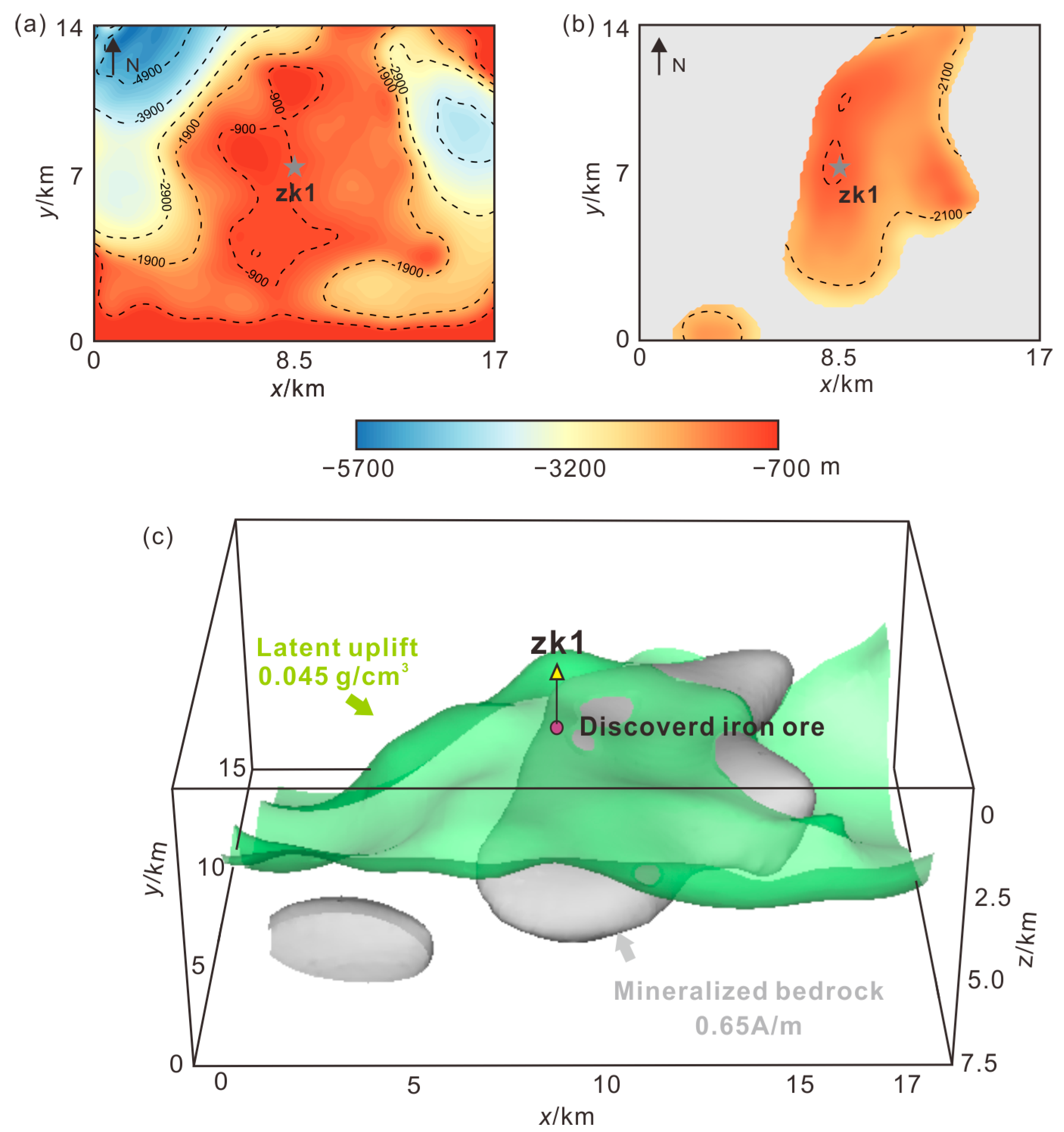
4.3. Real Data Inversion and Interpretation

In order to obtain the undulation of the uplift and the shape of the mineralized bedrock, the PTSS method with n = 3 has been utilized to jointly invert the Bouguer gravity and RTP magnetic data, resulting in the extraction of density and magnetization structures from the surface to 7.5 km depth within the study area. The exploration space was partitioned into 78 × 64 × 30 cells based on the sampling interval of the data, with each cell measuring 250 m × 250 m × 250 m in dimension. Furthermore, to mitigate the boundary effect of the inversion, five cells were externally extended in every direction. Figure 10 shows the inversion results of the east–west profile passing through the borehole. A density isosurface of 0.045 g/cm³ (shown as a lavender dotted line in Figure 10) is used as the upper interface of the uplift based on the depth of 900 m, as revealed by the borehole.

The undulating configuration of the uplift has been clearly discerned through the analysis of density results, with the thickness of the overlying Neogene–Quaternary layer observed to fluctuate between 1.0 and 1.4 km. Depressions are located to the east and west of the uplift, with the thickness of the covering layer thickening to 2.5 km. As a result of magnetic inversion, the shape and position of the mineralized bedrock are well identified. The shape of the bedrock is a sub-triangular shape dipping to the east with an average thickness of 2km, and it is located on the east side of the uplift and is adjacent to the east fault. The presence of intrusions can also be observed in the density inversion, but their boundaries are significantly not as well defined as in the magnetic results. The bedrock boundaries, as indicated by a magnetization isosurface of 0.65 A/m (shown as a red dotted line in Figure 10), are determined based on the depth of 1127 m revealed by the borehole. Magnetite was seen at a depth of 1145 m (deep purple asterisk in Figure 10).

Figure 11 presents the depth map (Figure 11a,b) and a three-dimensional view (Figure 11c) of the bedrock and upper interface of uplift. As can be seen, the intrusion as a whole is located on the eastern side of the uplift. Hence, during the Yanshanian movement, the magma intruded upward along the eastern rift, resulting in the formation of an intermediate–basic intrusion mass. This mass came into contact with and was responsible for the Mesozoic limestone layer, ultimately leading to the creation of a skarn-type iron ore deposit. It can be seen from Figure 11 that the intrusion as a whole lies on the eastern side of the uplift. However, the upper interface of the northern part of the bedrock is slightly higher than that of the uplift, while the depths of the two upper interfaces are similar in the west. It implies that the eastern part of the intrusion may have penetrated the Paleozoic dolomitic limestone layer, making it more difficult to form skarn-type deposits, while the southern part is a more favorable area for mineralization.

5. Conclusions

In this paper, the power-type structural self-constrained inversion (PTSS) methods are proposed to improve the resolution in smooth inversion. A self-constraint term, constructed by the gradient power of the initial result, is formed and has been introduced in the smoothing inversion to enhance the convergence of the result by strengthening the constraints at the boundary locations of the model and weakening the constraints at other locations. In the joint inversion, the power-type structural mutual-constrained term has been built with the gradient power of the respective initial results to enhance the mutual constraint between different physical structures. In addition, the self-constrained term can be incorporated into the inversion process to further enhance the resolution and maintain the structural features of respective inversion results. The synthetic model test results indicate that the PTSS inversion methods have high resolution compared with smooth inversion, and they have good anti-noise capability.

The PTSS joint method is applied to the joint inversion of airborne gravity and magnetic data in the iron ore district in Shandong, China. Our method clearly reveals the location and shape of uplift and mineralized bedrock. The inversion results correspond well to the lithology of the drill holes, proving the accuracy and good application prospects of the inversion method.

References

1. Nabighian, M.N.; Ander, M.E.; Grauch, V.J.S.; Hansen, R.O.; LaFehr, T.R.; Li, Y.; Pearson, W.C.; Peirce, J.W.; Phillips, J.D.; Ruder, M.E. Historical development of the gravity method in exploration. Geophysics 2005, 70, 63ND–89ND. [Google Scholar] [CrossRef]
2. Moazam, S.; Aghajani, H.; Kalate, A.N. The priority of microgravity focusing inversion in 3D modeling of subsurface voids. Environ. Earth Sci. 2021, 80, 343. [Google Scholar] [CrossRef]
3. Lü, Q.T.; Qi, G.; Yan, J.Y. 3D geologic model of Shizishan ore field constrained by gravity and magnetic interactive modeling: A case history. Geophysics 2013, 78, B25–B35. [Google Scholar] [CrossRef]
4. Zhang, M.H.; Xu, D.S.; Chen, J.W. Geological structure of the yellow sea area from regional gravity and magnetic interpretation. Appl. Geophys. 2007, 4, 75–83. [Google Scholar] [CrossRef]
5. Tikhonov, A.N.; Arsenin, V.I. Solutions of Ill-Posed Problems; Wiley: Hoboken, NJ, USA, 1977. [Google Scholar]
6. Li, Y.; Oldenburg, D.W. 3-D inversion of gravity data. Geophysics 1998, 63, 109–119. [Google Scholar] [CrossRef]
7. Boulanger, O.; Chouteau, M. Constraints in 3D gravity inversion. Geophys. Prospect. 2001, 49, 265–280. [Google Scholar] [CrossRef]
8. Farquharson, C.G. Constructing piecewise-constant models in multidimensional minimum-structure inversions. Geophysics 2007, 73, K1–K9. [Google Scholar] [CrossRef]
9. Rezaie, M.; Moradzadeh, A.; Kalate, A.N.; Aghajani, H. Fast 3D Focusing Inversion of Gravity Data Using Reweighted Regularized Lanczos Bidiagonalization Method. Pure Appl. Geophys. 2017, 174, 359–374. [Google Scholar] [CrossRef]
10. Last, B.J.; Kubik, K. Compact gravity inversion. Geophysics 1983, 48, 713–721. [Google Scholar] [CrossRef]
11. Portniaguine, O.; Zhdanov, M.S. Focusing geophysical inversion images. Geophysics 1999, 64, 874–887. [Google Scholar] [CrossRef]
12. Pilkington, M. 3D magnetic data-space inversion with sparseness constraints. Geophysics 2008, 74, L7–L15. [Google Scholar] [CrossRef]
13. Rezaie, M. A sigmoid stabilizing function for fast sparse 3D inversion of magnetic data. Near Surf. Geophys. 2020, 18, 149–159. [Google Scholar] [CrossRef]
14. Rezaie, M. 3D non-smooth inversion of gravity data by zero order minimum entropy stabilizing functional. Phys. Earth Planet. Inter. 2019, 294. [Google Scholar] [CrossRef]
15. Rezaie, M. Focusing inversion of gravity data with an error function stabilizer. J. Appl. Geophys. 2023, 208, 104890. [Google Scholar] [CrossRef]
16. Capriotti, J.; Li, Y. Gravity and gravity gradient data: Understanding their information content through joint inversions. In SEG Technical Program Expanded Abstracts; SEG: Houston, TX, USA, 2014; pp. 1329–1333. [Google Scholar]
17. Qin, P.; Huang, D.; Yuan, Y.; Geng, M.; Liu, J. Integrated gravity and gravity gradient 3D inversion using the non-linear conjugate gradient. J. Appl. Geophys. 2016, 126, 52–73. [Google Scholar] [CrossRef]
18. Capriotti, J.; Li, Y. Joint inversion of gravity and gravity gradient data: A systematic evaluation. Geophysics 2022, 87, G29–G44. [Google Scholar] [CrossRef]
19. Ma, G.; Gao, T.; Li, L.; Wang, T.; Niu, R.; Li, X. High-Resolution Cooperate Density-Integrated Inversion Method of Airborne Gravity and Its Gradient Data. Remote Sens. 2021, 13, 4157. [Google Scholar] [CrossRef]
20. Ma, G.; Zhao, Y.; Xu, B.; Li, L.; Wang, T. High-Precision Joint Magnetization Vector Inversion Method of Airborne Magnetic and Gradient Data with Structure and Data Double Constraints. Remote Sens. 2022, 14, 2508. [Google Scholar] [CrossRef]
21. Gallardo, L.A.; Meju, M.A. Characterization of heterogeneous near-surface materials by joint 2D inversion of dc resistivity and seismic data. Geophys. Res. Lett. 2003, 30. [Google Scholar] [CrossRef]
22. Zhou, J.; Meng, X.; Guo, L.; Zhang, S. Three-dimensional cross-gradient joint inversion of gravity and normalized magnetic source strength data in the presence of remanent magnetization. J. Appl. Geophys. 2015, 119, 51–60. [Google Scholar] [CrossRef]
23. Gallardo, L.A.; Meju, M.A. Joint two-dimensional DC resistivity and seismic travel time inversion with cross-gradients constraints. J. Geophys. Res. Solid Earth 2004, 109. [Google Scholar] [CrossRef]
24. Fregoso, E.; Gallardo, L.A. Cross-gradients joint 3D inversion with applications to gravity and magnetic data. Geophysics 2009, 74, L31–L42. [Google Scholar] [CrossRef]
25. Meng, Q.; Ma, G.; Li, L.; Wang, T.; Han, J. 3-D Cross-Gradient Joint Inversion Method for Gravity and Magnetic Data with Unstructured Grids Based on Second-Order Taylor Formula: Its Application to the Southern Greater Khingan Range. IEEE Trans. Geosci. Remote Sens. 2022, 60, 5914816. [Google Scholar] [CrossRef]
26. Moorkamp, M.; Heincke, B.; Jegen, M.; Roberts, A.W.; Hobbs, R.W. A framework for 3-D joint inversion of MT, gravity and seismic refraction data. Geophys. J. Int. 2011, 184, 477–493. [Google Scholar] [CrossRef]
27. Shi, B.; Yu, P.; Zhao, C.; Zhang, L.; Yang, H. Linear correlation constrained joint inversion using squared cosine similarity of regional residual model vectors. Geophys. J. Int. 2018, 215, 1291–1307. [Google Scholar] [CrossRef]
28. Paasche, H.; Tronicke, J. Cooperative inversion of 2D geophysical data sets: A zonal approach based on fuzzy c-means cluster analysis. Geophysics 2007, 72, A35–A39. [Google Scholar] [CrossRef]
29. Chen, J.; Hoversten, G.M. Joint inversion of marine seismic AVA and CSEM data using statistical rock-physics models and Markov random fields. Geophysics 2012, 77, R65–R80. [Google Scholar] [CrossRef]
30. Zhdanov, M.S.; Gribenko, A.; Wilson, G. Generalized joint inversion of multimodal geophysical data using Gramian constraints. Geophys. Res. Lett. 2012, 39. [Google Scholar] [CrossRef]
31. Lin, W.; Zhdanov, M.S. The Gramian Method of Joint Inversion of the Gravity Gradiometry and Seismic Data. Pure Appl. Geophys. 2019, 176, 1659–1672. [Google Scholar] [CrossRef]
32. Zhdanov, M.S.; Jorgensen, M.; Tao, M. Probabilistic approach to Gramian inversion of multiphysics data. Front. Earth Sci. 2023, 11, 1127597. [Google Scholar] [CrossRef]
33. Kong, R.J.; Hu, X.Y.; Cai, H.Z. Three-dimensional joint inversion of gravity and magnetic data using Gramian constraints and Gauss-Newton method. Chin. J. Geophys. Chin. Ed. 2023, 66, 3493–3513. [Google Scholar] [CrossRef]
34. Jiao, J.; Dong, S.; Zhou, S.; Zeng, Z.; Lin, T. 3-D Gravity and Magnetic Joint Inversion Based on Deep Learning Combined with Measurement Data Constraint. IEEE Trans. Geosci. Remote Sens. 2024, 62, 5900814. [Google Scholar] [CrossRef]
35. Zhang, Z.H.; Liao, X.L.; Cao, Y.Y.; Hou, Z.L.; Fan, X.T.; Xu, Z.X.; Lu, R.Q.; Feng, T.; Yao, Y.; Shi, Z.Y. Joint gravity and gravity gradient inversion based on deep learning. Chin. J. Geophys. Chin. Ed. 2021, 64, 1435–1452. [Google Scholar] [CrossRef]
36. Hu, Y.Y.; Wei, X.L.; Wu, X.Q.; Sun, J.J.; Chen, J.P.; Huang, Y.Q.; Chen, J.F. A deep learning-enhanced framework for multiphysics joint inversion. Geophysics 2023, 88, K13–K26. [Google Scholar] [CrossRef]
37. Aster, R.; Borchers, B.; Thurber, C. Parameter Estimation and Inverse Problem; Academic Press: New York, NY, USA, 2005. [Google Scholar]
38. Menke, W. Geophysical Data Analysis: Discrete Inverse Theory (MATLAB Edition); Academic Press: London, UK, 2012. [Google Scholar]
39. Camacho, A.G.; Montesinos, F.G.; Vieira, R. Gravity inversion by means of growing bodies. Geophysics 1999, 65, 95–101. [Google Scholar] [CrossRef]
40. Krahenbuhl, R.A.; Li, Y. Inversion of gravity data using a binary formulation. Geophys. J. Int. 2006, 167, 543–556. [Google Scholar] [CrossRef]
41. Krahenbuhl, R.A.; Li, Y. Hybrid optimization for lithologic inversion and time-lapse monitoring using a binary formulation. Geophysics 2009, 74, I55–I65. [Google Scholar] [CrossRef]
42. Lelièvre, P.G.; Oldenburg, D.W. A comprehensive study of including structural orientation information in geophysical inversions. Geophys. J. Int. 2009, 178, 623–637. [Google Scholar] [CrossRef]
43. Li, Y.; Oldenburg, D.W. Incorporating geological dip information into geophysical inversions. Geophysics 2000, 65, 148–157. [Google Scholar] [CrossRef]
44. Zhou, J.; Revil, A.; Karaoulis, M.; Hale, D.; Doetsch, J.; Cuttler, S. Image-guided inversion of electrical resistivity data. Geophys. J. Int. 2014, 197, 292–309. [Google Scholar] [CrossRef]
45. Blakely, R.J. Potential Theory in Gravity and Magnetic Applications; Cambridge University Press: Cambridge, UK, 1996. [Google Scholar]
46. Hansen, P.C.; O’Leary, D.P. The Use of the L-Curve in the Regularization of Discrete Ill-Posed Problems. SIAM J. Sci. Comput. 1993, 14, 1487–1503. [Google Scholar] [CrossRef]
47. Hao, X.Z.; Yang, Y.H.; Li, Y.P.; Gao, L.H.; Chen, L. Ore-controlling Characteristics and Prospecting criteria of iron deposits in Qihe area of Western Shandong. J. Jilin Univ. Earth Sci. Ed. 2019, 49, 982–991. [Google Scholar]
48. Gao, X.; Xiong, S.; Yu, C.; Zhang, D.; Wu, C. The Estimation of Magnetite Prospective Resources Based on Aeromagnetic Data: A Case Study of Qihe Area, Shandong Province, China. Remote Sens. 2021, 13, 1216. [Google Scholar] [CrossRef]
49. Wu, C.P.; Yu, C.C.; Wang, W.P.; Ma, X.B.; Fan, Z.G.; Zhu, H.W. Physical characteristics of rocks and ores and their application in Qihe area, Western Shandong. Adv. Earth Sci. 2019, 34, 1099–1107. [Google Scholar]
50. Wu, C.P.; Yu, C.C.; Zhou, M.L.; Wang, W.P.; Ma, X.B.; Li, S.Q. Residual calculation of airborne and ground magnetic field and its prospecting application in heavily covered plain area. Prog. Geophys. 2020, 35, 663–668. [Google Scholar]
51. Zhu, Y.Z.; Zhou, M.L.; Gao, Z.J.; Zhang, X.B. The discovery of the Qihe-Yucheng skarn type rich iron deposit in Shandong and its exploration significance. Geol. Bull. China 2018, 37, 938–944. [Google Scholar]
52. Wang, W.P.; Wu, C.P.; Ma, X.B. Aeromagnetic field feature and iron ore target prospecting in deep coverage area of Qihe in Shandong Province. Geol. Surv. China 2020, 7, 23–29. [Google Scholar]
Figure 1. Structural self-contained inversion strategies. (a) Respective inversion and (b) joint inversion.
Remotesensing 16 00681 g001
Figure 2. (a) Three-dimensional location of simple prism model; (b) gravity data for the model.
Remotesensing 16 00681 g002
Figure 3. (a) Three-dimensional location of double anomalous bodies model, (b) noisy gravity data, and (c) magnetic data for the model.
Remotesensing 16 00681 g003
Figure 4. Geological structure diagram of Qihe area.
Remotesensing 16 00681 g004
Figure 5. (a) Bourger gravity anomalies and (b) RTP magnetic anomalies from airborne geophysical surveys (The gray asterisk represents the drilling hole zk1).
Remotesensing 16 00681 g005
Figure 6. Vertical slices of the inversion results for simple prism model at y = 5 km. (a) Smooth inversion; PTSS inversion with powers of physical gradient n = 1 (b), n = 2 (c), and n = 3 (d).
Remotesensing 16 00681 g006
Figure 7. Vertical slices and 3D views of the inversion results for double anomalous bodies model at y = 5 km. (a,b) Smooth inversion; PTSS inversion with power of physical gradient n = 1 (c,d), n = 2 (e,f), and n = 3 (g,h).
Remotesensing 16 00681 g007
Figure 8. Vertical slices of result of gravity and magnetic data joint inversion (only introduce the structural mutual-constrained term) at y = 5 km. (a) Density result of smooth inversion; (b) magnetization result of smooth inversion; (c) density result of PTSS joint inversion with n = 1; (d) magnetization result of PTSS joint inversion with n = 1; (e) density result of PTSS joint inversion with n = 2 (f) magnetization result of PTSS joint inversion with n = 2; (g) density result of PTSS joint inversion with n = 3; (h) magnetization result of PTSS joint inversion with n = 3.
Remotesensing 16 00681 g008
Figure 9. Vertical slices of result of PTSS joint inversion (Introducing structural mutual-constrained and self-constrained terms). (a) Density result of PTSS joint inversion with n = 1; (b) magnetization result of PTSS joint inversion with n = 1; (c) density result of PTSS joint inversion with n = 2 (d) magnetization result of PTSS joint inversion with n = 2; (e) density result of PTSS joint inversion with n = 3; (f) magnetization result of PTSS joint inversion with n = 3.
Remotesensing 16 00681 g009
Figure 10. Vertical profile passing through PTSS joint inversion results: (a) density; (b) magnetization.
Remotesensing 16 00681 g010
Figure 11. (a) Depth of the uplift upper interface; (b) depth of the bedrock; (c) three-dimensional view of uplift upper interface and bedrock (The gray asterisk represents the drilling hole zk1).
Remotesensing 16 00681 g011
Disclaimer/Publisher’s Note: The statements, opinions and data contained in all publications are solely those of the individual author(s) and contributor(s) and not of MDPI and/or the editor(s). MDPI and/or the editor(s) disclaim responsibility for any injury to people or property resulting from any ideas, methods, instructions or products referred to in the content.