1. Introduction
The rapid advancement of Internet of Things (IoT) technology has catalyzed an unprecedented surge in data generation. Recent projections indicate that the number of active IoT devices may approach 30 billion by 2030 [
1]. Despite extensive mobile network deployment, connectivity remains elusive in many remote areas, such as deserts or oceans. This connectivity gap is underscored by research indicating that terrestrial wireless networks cover merely 20% of the global land area and less than 6% of the Earth’s surface [
2]. This limited reach is attributed to challenging terrain, extended communication distances, and various commercial and engineering complexities. In light of these limitations, there is a consensus among academic and industrial experts on the necessity of Satellite Communication (SatCom) networks as an effective supplement to terrestrial infrastructures. SatCom is deemed crucial for achieving comprehensive global coverage and facilitating seamless connectivity, particularly for critical computing applications like artificial intelligence (AI) [
3].
Over the last five decades, the cellular network landscape has undergone a rapid transformation, evolving from the First Generation to the cutting-edge Fifth Generation Mobile Network. Currently, the technological frontier is shifting towards the exploration of the Sixth Generation (6G) of communication technology, which is poised to play a pivotal role in the Smart Information Society envisioned for 2030 [
4]. Anticipated to outperform its predecessor, 6G is expected to cater to a plethora of emerging services and applications, marking a significant leap in communication technology [
5,
6]. The Sixth Generation is expected to revolutionize network coverage and user mobility by optimizing infrastructures in the air, in space, on the ground, and at sea. It aims to seamlessly integrate terrestrial and non-terrestrial networks, thus offering comprehensive and unrestricted coverage [
7,
8].
Concurrently, the surge in data produced by ubiquitous IoT devices has necessitated the application of AI techniques, such as deep learning, for the development of sophisticated data models. These models are integral to smart IoT applications in healthcare, transportation, and urban management [
9]. Traditionally, AI processing has been centralized in cloud servers or data centers [
10], a practice that faces significant challenges in the era of IoT data proliferation. Centralized data collection and transmission are often impractical or inefficient due to communication resource constraints and latency issues. Moreover, the sensitivity of the massive data generated raises significant security concerns, as highlighted by global regulatory frameworks like the General Data Protection Regulation in Europe [
11].
Federated learning (FL), a pioneering distributed machine learning framework, was introduced by Google in 2016. As a technical paradigm, FL represents a distributed, collaborative form of AI. It enables multiple devices to coordinate with a central server for data training purposes, without necessitating the sharing of the actual dataset [
12]. FL is distinguished by several key advantages, including improved communication efficiency and enhanced data privacy. These benefits stem from its ability to transmit only model parameters instead of raw data [
13].
In the realm of next-generation wireless communications, particularly those encompassing the Space-Air-Ground Information Network (SAGIN) augmented by AI, FL has garnered significant research interest. This interest is propelled by the expanding integration and prevalence of data-driven applications. However, the financial viability of SatCom, when compared with that of terrestrial mobile networks, remains a concern. To facilitate intelligent adaptive learning for extensive IoT networks and to mitigate the costs associated with high-volume SatCom traffic, recent studies have explored the application of FL within low-Earth-orbit SatCom networks [
14].
Previous research has delved into enhancing wireless network efficiency, focusing on Mobile Edge Computing (MEC) and federated learning (FL). In MEC, studies have addressed energy-efficient task offloading challenges in Layer 2 Service Chaining services across multi-Radio Access Technology networks, considering constraints like stringent latency and residual battery energy [
15,
16]. For FL in wireless networks, a novel model has been proposed to optimize base station resource allocation and user transmission power allocation, jointly considering learning and wireless network metrics. This aims to reduce packet error rates and enhance overall FL performance [
17].
To overcome challenges in the Metaverse’s channel state and computing resources, a soft actor–critic-based solution has been developed for an efficient FL scheme with dynamic user selection, gradient quantization, and resource allocation [
18]. Recognizing the limitations of asynchronous federated learning and semi-asynchronous federated learning methods, a new approach named FedSEA has been introduced as a semi-asynchronous FL framework tailored for extremely heterogeneous devices [
19]. Additionally, in vehicular networking scenarios, studies have applied fuzzy logic for client selection, considering parameters such as the number and freshness of local samples, computational capability, and available network throughput [
20].
Nevertheless, most of the existing works rely on an unrealistic assumption that edge devices participating in federated training have stable network connections [
21,
22]. In practice, the network quality may change due to the movement of devices or the change in environmental factors. Unpredictable network quality increases the difficulty of designing FL algorithms. Meanwhile, mobile industrial devices using battery power [
23] in this scenario usually have limited computational and communication resources. This also puts a higher demand on the time and energy consumption of joint training. Some existing solutions employ a Deep Deterministic Policy Gradient (DDPG) to address latency and energy consumption issues when selecting FL participants among IoT device nodes [
24,
25].
In this paper, we model the delay and energy consumption for each round of federated training. Under the condition of independent and identically distributed data distribution, the Low-Cost Node Selection in Federated Learning (LCNSFL) algorithm, based on the Double Deep Q Network (DDQN), is proposed to minimize the time and energy consumption of each round of federation training. This algorithm aims to minimize the time and energy consumption associated with each training round. LCNSFL assists the edge server in selecting the most efficient device set for participation in federated training, leveraging the system state information collected. Through comparative experimental analysis, we demonstrate that LCNSFL significantly reduces both time and energy consumption in federated training while ensuring high convergence accuracy of the global model.
The rest of the paper is organized as follows:
Section 2 models the latency and energy consumption of the federated training process. In
Section 3, we design the node selection algorithm for minimizing training consumption in DDQN-based FL.
Section 4 evaluates the algorithm, and
Section 5 concludes the paper. All acronyms used throughout this survey paper are given in
Table 1.
2. System Model and Problem Definition
In the paper, we investigate the time and energy consumption of FL with various IoT devices and time-varying channel state information. First, the time and energy consumption are defined. Then, the nodes are selected to minimize the consumption in each federated training step. Finally, a DDQN-based algorithm is proposed to solve the formulated problem.
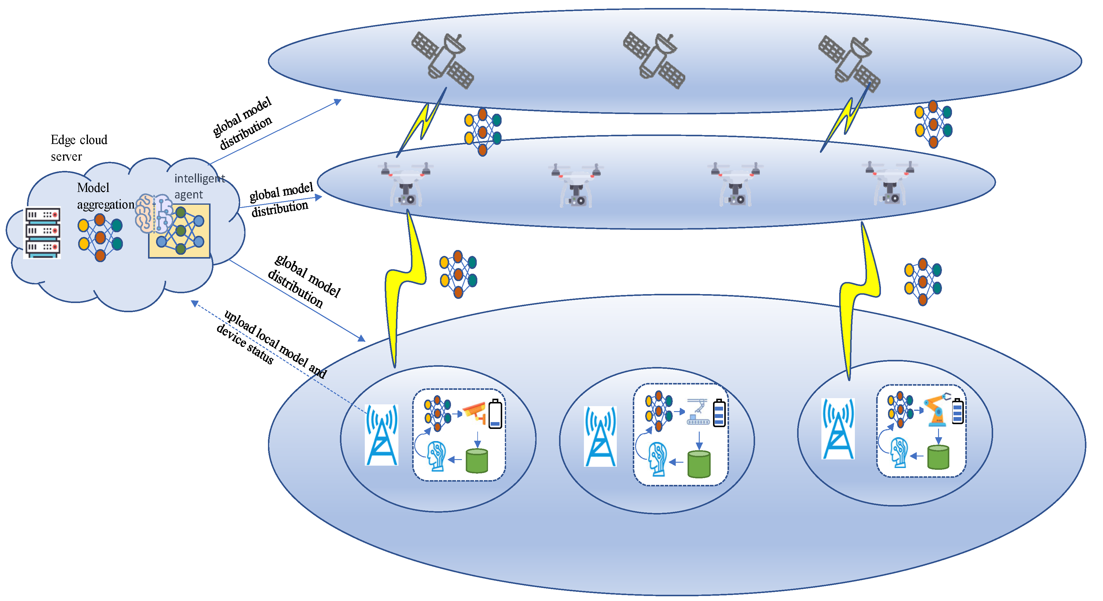
As depicted in
Figure 1, the architecture of the Distributed Reinforcement Learning (DRL)-enhanced FL system is presented for implementation in the SAGIN. The SAGIN encompasses satellites, Unmanned Aerial Vehicles (UAVs), and ground base stations. The IoT devices refer to cameras and robotic arms, etc., which establish connections to the edge cloud server. To achieve the federated averaging scheme, these devices first transmit the local model parameters to the edge cloud server, and then the edge cloud server aggregates those parameters. These aggregated algorithms are employed to update the global federation model. It should be noted that this process in a server can be augmented with a Reinforcement Learning Intelligence (RLI) component. The RLI aids the FL system by strategically selecting a subset of devices to partake in the federation training.
Prior to the initiation of each round of federated training, the edge cloud server carefully selects a subset of IoT devices to actively participate in the training process, delivering to them the latest iteration of the global model. The designated IoT devices leverage locally available data for model training and subsequently transmit the refined model parameters back to the edge cloud server. Following this, the edge cloud server undertakes the essential task of parameter aggregation, systematically iterating through the aforementioned steps until the accuracy of the global model reaches the predefined target.
The time and energy requirements for each round of federated training can be categorized into three components: computational time for local model training, duration of data transmission, and idle waiting periods for devices. Similarly, IoT device energy consumption during training includes computational energy, energy required for parameter transmission, and energy consumed during idle waiting.
Due to the superior communication resources available to the edge cloud server, whose downstream bandwidth significantly exceeds that of the upstream bandwidth of industrial IoT devices, the time and energy requirements for devices to download the global model in each training round may be reasonably overlooked.
We can integrate energy consumption sensors on each IoT device node to monitor real-time power consumption. With the data collected from these sensors, we can quantify the energy consumption of each node under various tasks. However, it is not feasible for the server to obtain the local training time and energy consumption of all devices in advance before the start of a federated training round. Therefore, designing a node selection strategy to avoid high-energy-consuming devices and those with poor channel quality from participating in the federated training process will help reduce the time and energy consumption of the federated training process. This is crucial for resource-constrained IoT devices.
This paper focuses on FL algorithm design for node selection without considering the optimization of the DDQN network architecture. Key symbols in this study are listed in
Table 2.
The FL system consists of an edge server (ES) and N IoT devices. The devices are denoted by an index i: i ∈ S, S = {1, 2, …, N}. The dataset of device i is represented as Di, and its size is denoted as di. (xi, yi) represents a data sample from Di, where xi denotes the sample data and yi represents the sample label. During local model training, xi is used as the input to the model, and yi is used as the expected output. The cross-entropy between yi and the model’s predicted output yi’ is calculated as the local model’s loss function.
Figure 2 illustrates the scheduling process of federated synchronous learning. Prior to the commencement of each FL round, the ES selects
n devices to participate in the training process. The set of selected devices is represented as
Ssub, where
Ssub = {1, 2, …,
n}. The ES distributes the global model to each selected device, which then performs τ iterations to update the model using its local dataset
Di. After completing local model training, each device uploads its local model’s weight parameters to the ES. The ES performs the model aggregation algorithm to obtain the latest global model and then proceeds to the next round of federated training.
Assuming that device
i requires
ci CPU cycles to train a single sample and operates at a frequency of
fi, the computation time required for device
i to execute local model training in the
k-th round of federated training is given by
After completing the local model updates, device
i uploads the trained model’s weight parameters
to the ES. The transmission time of the model is calculated using the following formula:
where |
| represents the size of the model weights,
represents the data transmission rate of device
i in the
k-th round of federated training, and
is calculated using the following equation:
The transmission signal of the UAV system in the SAGIN is affected by various fading effects in the ground-to-space channel, including large-scale path fading, shadow fading, and small-scale fading. To address this, a generalized CE2R channel model is introduced. In this model, A is a constant and is the path loss index. It is a general form of the path loss model, and parameter adjustments are required on a case-by-case basis [
26].
According to the above equation, the data transmission rate of device
i is influenced by the allocated bandwidth to device
i (
), the transmission power of device
i (
), the channel gain (
), and the noise power (
N0). Changes in environmental conditions can affect the data transmission rate and introduce uncertainty in transmission delays. The training time of device
i in the
k-th round of federated training is the sum of the computation time for local model updates and the model transmission time. Therefore, the training time of device
i can be obtained using the following equation:
In the federated synchronous model, the next round of federated training begins only when the ES receives the local model parameters from all devices and creates a new global model. Therefore, the learning time of the
k-th round of federated training is determined by the slowest device, and it can be represented by the following formula:
According to the energy model proposed in reference [
27], the energy consumed by device
i during local model training in the
k-th round of federated training can be calculated using the following equation:
where
represents the effective capacitance coefficient, which is related to the properties of the chip itself.
During model transmission, device
i performs the model transmission with a power of
. Therefore, the energy consumption of device
i for transmission is calculated as
The device that completes local model training and model transmission first needs to wait for other devices that have not finished. Fast devices may experience idle waiting time, and the energy consumed during this idle waiting period is referred to as idle energy consumption. Therefore, the idle energy consumption of device
i is equal to the product of idle waiting time and the energy consumption per unit time in the idle state. The calculation formula is as follows:
where
represents the energy consumption per unit time of device
i during the idle waiting period. Therefore, the total energy consumed by device
i during the
k-th round of federated training can be calculated as follows:
Therefore, the total energy consumed during the
k-th round of federated training can be calculated as follows:
Equations (11)–(17) describe the device selection problem under the independent and identically distributed data distribution. It can be formulated as selecting a group of devices in each round of federated training to minimize the training time consumption and energy consumption cost. To reduce the idle waiting time of fast devices and minimize unnecessary idle energy consumption, the selected devices must have similar training time costs. This problem can be formulated as the minimization of
Tk. The formulation of the optimization problem is as follows:
Due to different requirements of different FL tasks for the latency and energy consumption in each training round, a trade-off between time cost and energy cost can be achieved by using the hyperparameter . In Equation (11), represents the preference for the optimization objective. If takes a relatively large value, it indicates that the optimization model focuses more on reducing energy consumption during training. If takes a relatively small value, the optimization model pays more attention to reducing training time cost. represents the decision variable, where = 1 indicates that device i is selected to participate in federated training in the k-th communication round, and = 0 indicates that device i does not participate in the federated training process. Equation (12) represents the constraint on device operating frequency. Devices with excessively high or low frequencies will not be selected, ensuring that the computational latency and computational energy consumption are not too large. Equation (13) represents the constraint that the total bandwidth of the selected devices should not exceed the server’s bandwidth. Equation (14) represents the constraint that at least one device should be selected to participate in federated training in a communication round, and the maximum number of selected devices does not exceed the total number of devices. Equation (15) is the constraint on the energy consumption of device i, which should not exceed a specified upper limit.
3. Design of Node Selection Algorithm for Minimum Training Cost in FL Based on DDQN
Due to the nonlinearity of the constraints and the unpredictable changes in the network states of each device, solving the optimization problem described in Equation (11) is extremely challenging. In order to find the optimal set of devices for each round of federated training and achieve a dynamic trade-off between time cost and energy cost, the DDQN algorithm is considered for solving the node selection problem. This node selection scheme is named LCNSFL.
To solve the node selection problem in FL using the DRL approach, it is first necessary to abstract the problem as a Markov Decision Process (MDP). An MDP consists of a system state S(t), an action space A(t), a policy π, a reward function r, and neighboring states S(t + 1). The detailed parameter description is as follows.
- (a)
System state: This chapter considers a practical scenario with dynamic network bandwidth. However, it is assumed that the network state remains relatively stable within a short time slot and does not undergo drastic changes within a few tens of seconds. The state space S(t) for DRL is defined as the combination of the device’s data transmission rate β(t), operating frequency ζ(t), signal transmission power Tp(t), and the number of samples owned by the device I(t). Thus, at time slot t, the system state can be represented by the following equation:
It is worth noting that due to the heterogeneity of devices and the instability of network conditions, the data transmission rate and operating frequency of each device may vary at different time slots t. Therefore, before each round of federated training, it is necessary to sample the data transmission rate, operating frequency, and other information of each device multiple times and take the average as the current state variables. On the other hand, the number of samples owned by each device and the signal transmission power are relatively stable, so the sampled values at time slot t can be used as the system’s state variables.
- (b)
The action space, denoted as A(t), is a vector consisting of discrete variables (0 or 1). represents the selection status of device i at time slot t. = 1 indicates that device i is selected to participate in federated training at time slot t, while = 0 indicates that device i does not participate in federated training at time slot t.
- (c)
The policy π represents the mapping from the state space S(t) to the action space A(t), i.e., A(t) = π(S(t)). The goal of DRL is to learn an optimal policy π that maximizes the expected reward based on the current state.
- (d)
The reward function r is aligned with the optimization objective, which is to minimize the weighted sum of time cost and energy cost. Therefore, the reward function r can be expressed as follows:
- (e)
The adjacent state S(t + 1) is determined based on the current state S(t) and the policy π. The specific expression is as follows:
It is important to note that the reward defined in Equation (19) is an immediate reward, i.e., the instantaneous reward feedback, denoted as rt, received from the environment after the agent takes action a(t) based on policy π at time t. The goal of DRL is to maximize the sum of immediate rewards and discounted future rewards. Based on the Bellman equation and temporal difference algorithm, to obtain the optimal policy using the value function approach in DRL, it is necessary to estimate the action-value function for future time steps and discount the action-value function for future time steps using a discount factor, γ. The temporal difference target is defined as , where Q(st, at) is the estimated action-value function at time t. Since rt is the true reward obtained at time t, it is considered more reliable than the estimate Q(st, at). Therefore, the goal is to approximate the action-value function estimated at time t to . The temporal difference error, , is optimized using loss functions such as mean square error to improve the accuracy of the neural network’s estimation of the state value.
The FL node selection problem is addressed by employing the DDQN reinforcement learning model on edge cloud servers, achieving a dynamic trade-off between energy consumption and training time. The DDQN algorithm, which is capable of processing continuous states and generating discrete actions through neural networks, is particularly well suited for addressing the node selection challenge in FL within IoT scenarios. In comparison with alternative algorithms such as DDPG, Trust Region Policy Optimization, and others, the DDQN strikes a favorable balance concerning algorithmic simplicity, sample complexity, and parameter tuning flexibility and mitigates the issue of Q-value overestimation observed in the standard Deep Q Network algorithm.
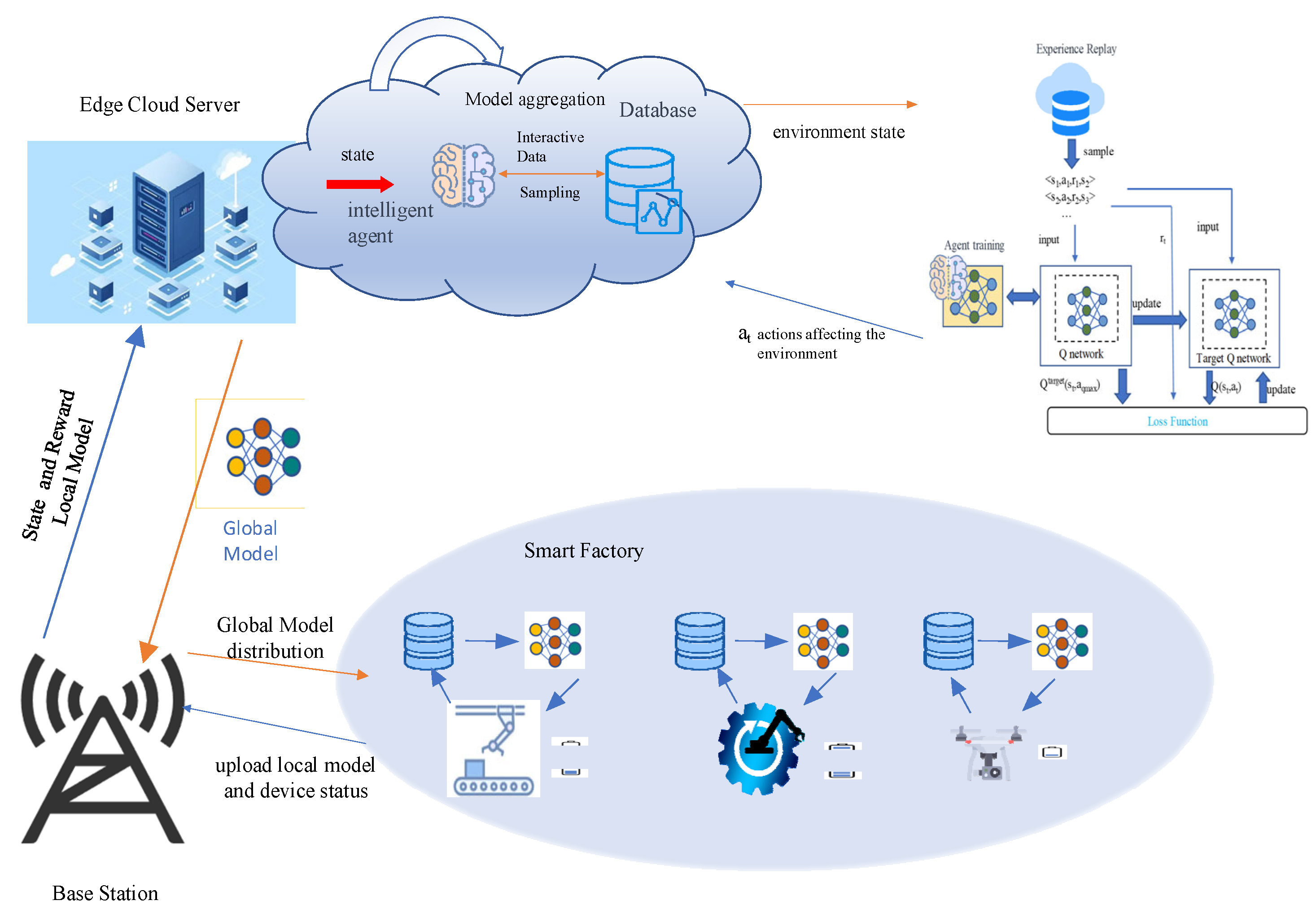
As shown in
Figure 3, edge cloud servers are usually deployed at edge locations close to production or sensing devices, such as factories or production lines, and are connected to IoT devices through base stations. Such a deployment can optimize the efficiency of data processing and decision making, reduce data transmission delays, and improve the real time and responsiveness of the system.
The DDQN algorithm consists of a Q network and a target Q network. For convenience’s sake, the target Q network is denoted as “target Q”. In order to compress the action space, during the training phase, the index corresponding to the maximum Q value output by the Q network at time t is selected as the device number for local model updates. This approach reduces the action space from 2N to N, where N is the total number of IoT devices. The Q network outputs the action at based on the current state st, which interacts with the FL environment. Subsequently, the state of the FL environment transitions from st to st+1, and a scalar is returned to the agent as an immediate reward, rt. A boolean variable “done” is defined as the termination flag for federated training. When the communication rounds of federated training reach the upper limit, “done” is set to true, and the training process is terminated. The tuple < st, at, rt, st+1, done > is stored in the experience replay buffer as a record of the interaction between the agent and the environment. When the interaction data in the experience replay buffer reach a certain quantity, the Q network trains on the data from the buffer, updating the node selection strategy.
The Q network is updated using a temporal difference algorithm. The state
st and action
at are inputted into the Q network, yielding the action value at time
t, denoted as
Q(st, at). Then, the next state
st+1 is inputted into the Q network to obtain the q values for different actions, and the action corresponding to the maximum q value, denoted as
amaxq, is selected. Next,
st+1 is inputted into the target Q network to find the q value corresponding to the action
amaxq, denoted as
Qtarget(
st+1, amaxq). Finally,
Q(
st, at) is used as the predicted value of the network, and
rt + γQtarget(
st+1, amaxq) is used as the actual value of the network. Mean square error is used as the loss function to perform backpropagation on
rt + γQtarget(
st+1,
amaxq) −
Q(
st,
at). To ensure the stability of the training process, in practice, only the parameters of the Q network are updated, while the weight parameters of the target Q network are fixed. The detailed training flow of the LCNSFL node selection algorithm is as follows (Algoritm 1):
| Algorithm 1. The training process of the FL node selection algorithm based on LCNSFL. |
| Input: Q network, target Q network Qtar, target network update frequency ftar, greedy factor e, greedy factor decay factor β, minimum sample size of the experience pool mBatch, maximum communication rounds of FL T, total number of devices N. |
| Output: The trained Q network Q and the trained target Q network Qtar. |
| 1: Initialize the local models of the devices, initialize the Q network as Q, initialize the target Q network as Qtar, and set the step counter as step = 0. |
| 2: for t = 1 to T do |
| 3: Collect the state s(t) |
| 4: done = False |
| 5: Generate a random number rd |
| 6: if rd > epsilon then |
| 7: a(t) = random(0,N) |
| 8: else |
| 9: a(t) = |
| 10: end if |
| 11: The edge server selects a device based on the action a(t), performs local model training on the selected device, and updates the global model. |
| 12: Compute the instantaneous reward r(t) based on Formula (19) and update the state from s(t) to s(t+1). |
| 13: if t = T then |
| 14: done = False |
| 15: end if |
| 16: Store the tuple information <s(t), a(t), r(t), s(t+1), done> in the experience pool. |
| 17: if the number of samples in the experience pool > mBatch then |
| 18: Randomly sample mBatch number of samples from the experience pool |
| 19: Use the Q network to estimate the q value Q(s(t), a(t)) at time t. |
| 20: Use the Q network to estimate the q value Q(s(t+1), a(t+1)) at time t+1 and obtain the action amaxq corresponding to the maximum q value. |
| 21: Use the target Q network to estimate the action value Qtar(s(t+1), amaxq) at time t + 1. |
| 22: Optimize the Q network based on the stochastic gradient descent (SGD) method using Formula (23). |
| 23: Update the greedy factor . |
| 24: if step%ftar = 0 then |
| 25: Update the parameters of the target Q network (Qtar) using the parameters of the Q network. |
| 26: end if |
| 27: step = step + 1 |
| 28: end if |
| 29: end for |
| 30: return the trained Q network Q and the trained target Q network Qtar. |
The DDQN algorithm separates action selection and value estimation. Specifically, it selects the action corresponding to the maximum q value at state
st+1 from the Q network, denoted as
a*. The value of action
a* at state
st+1 is estimated using the target Q network. The calculation of the TD target in the DDQN is expressed as follows:
During the training process, the parameters
θ− of the target Q network are frozen, meaning that the target Q network is not updated. The parameters of the Q network, denoted as
θ, are copied to
θ− every
freq iteration. The loss function of the Q network is defined as follows:
The update process of minimizing the loss function
through gradient descent is as follows for
θ:
The symbol α represents the step size or learning rate for the update.
5. Conclusions
The application of FL in SAGIN facilitates collaborative modeling among devices while ensuring the protection of endpoint device data privacy, providing a data-driven solution. However, challenges such as heterogeneous computational resources, fluctuating data transmission rates due to environmental factors, and limited energy resources significantly impact device selection during the federated training process.
In this study, we established models for time delay and energy consumption in the federated training process. Subsequently, we introduced the LCNSFL algorithm based on DDQN to minimize the time and energy costs in each round of federated training. The LCNSFL algorithm adaptively selects the optimal device subset by considering the collected device status information, achieving a dynamic trade-off between time cost and energy cost in federated training.
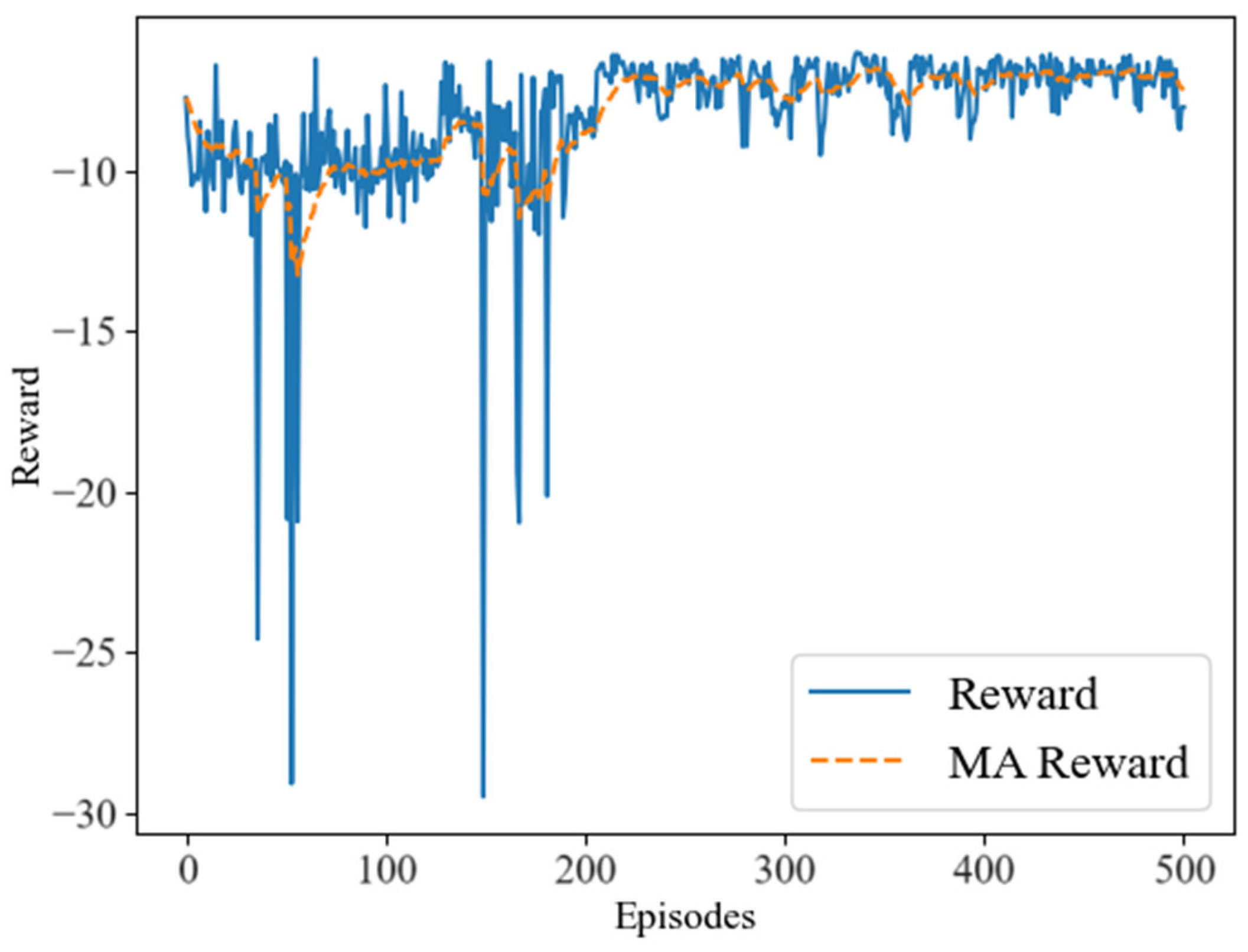
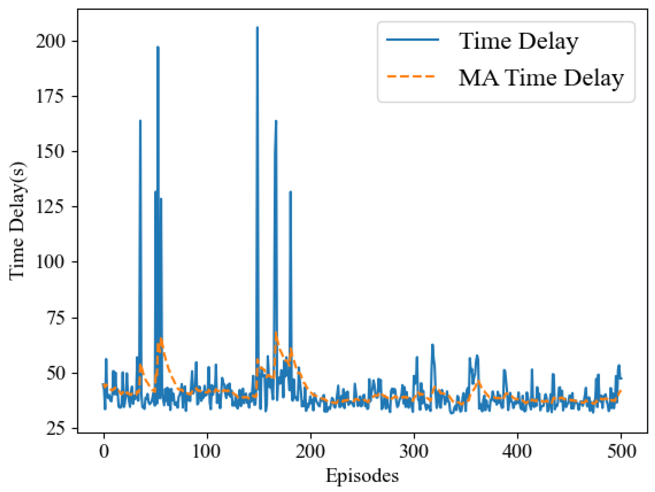
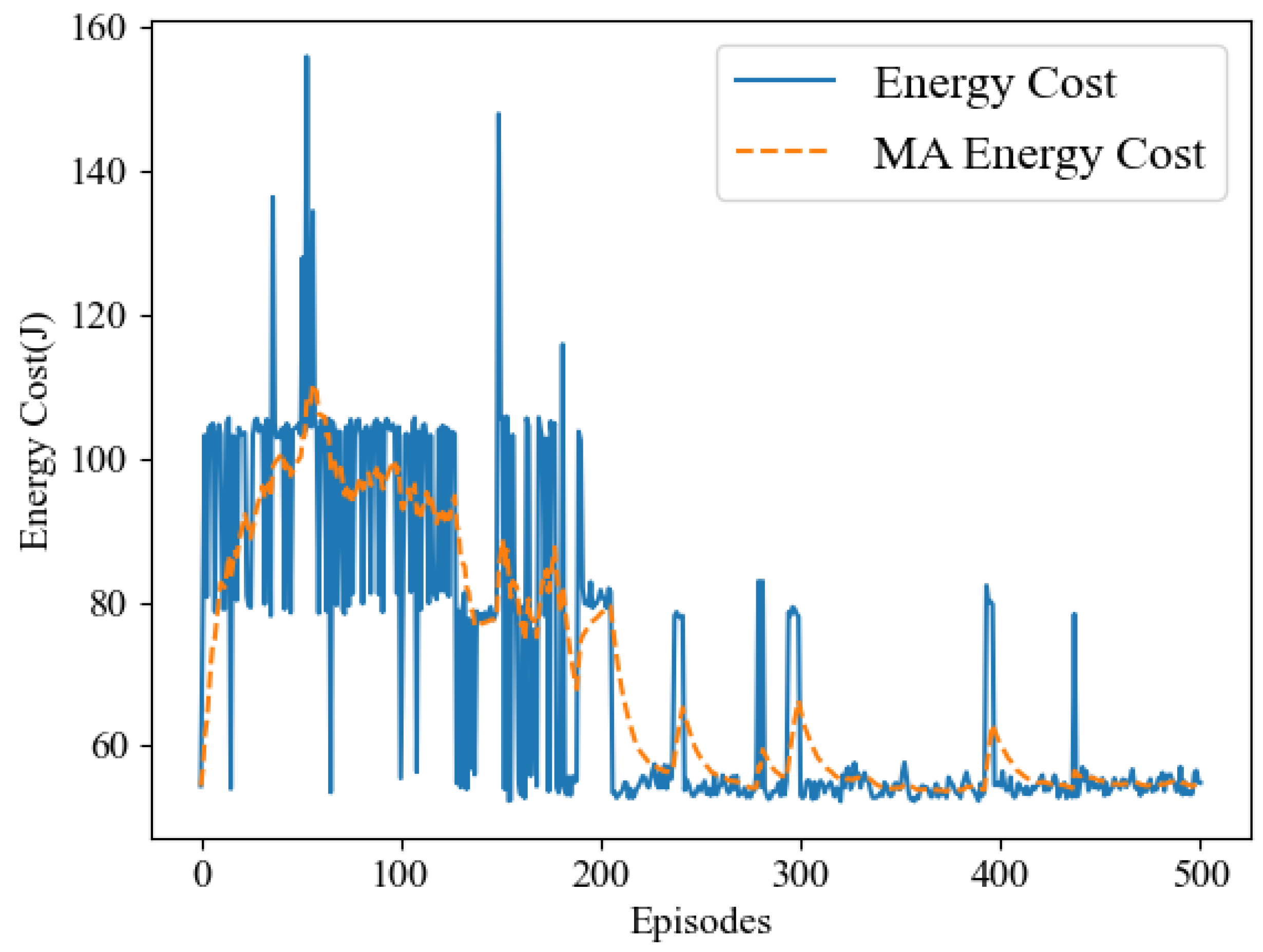
In our simulation experiments, we observed that the LCNSFL algorithm gradually increases rewards during the training phase and tends to converge after 400 rounds of iterations. The training loss also decreases gradually, reaching a relatively low level and stabilizing after 400 iterations, indicating effective convergence. Once the reward values converge, the DRL agent performs well in device selection tasks in the federated learning environment, and the time and energy costs of each round of federated training also tend to stabilize.
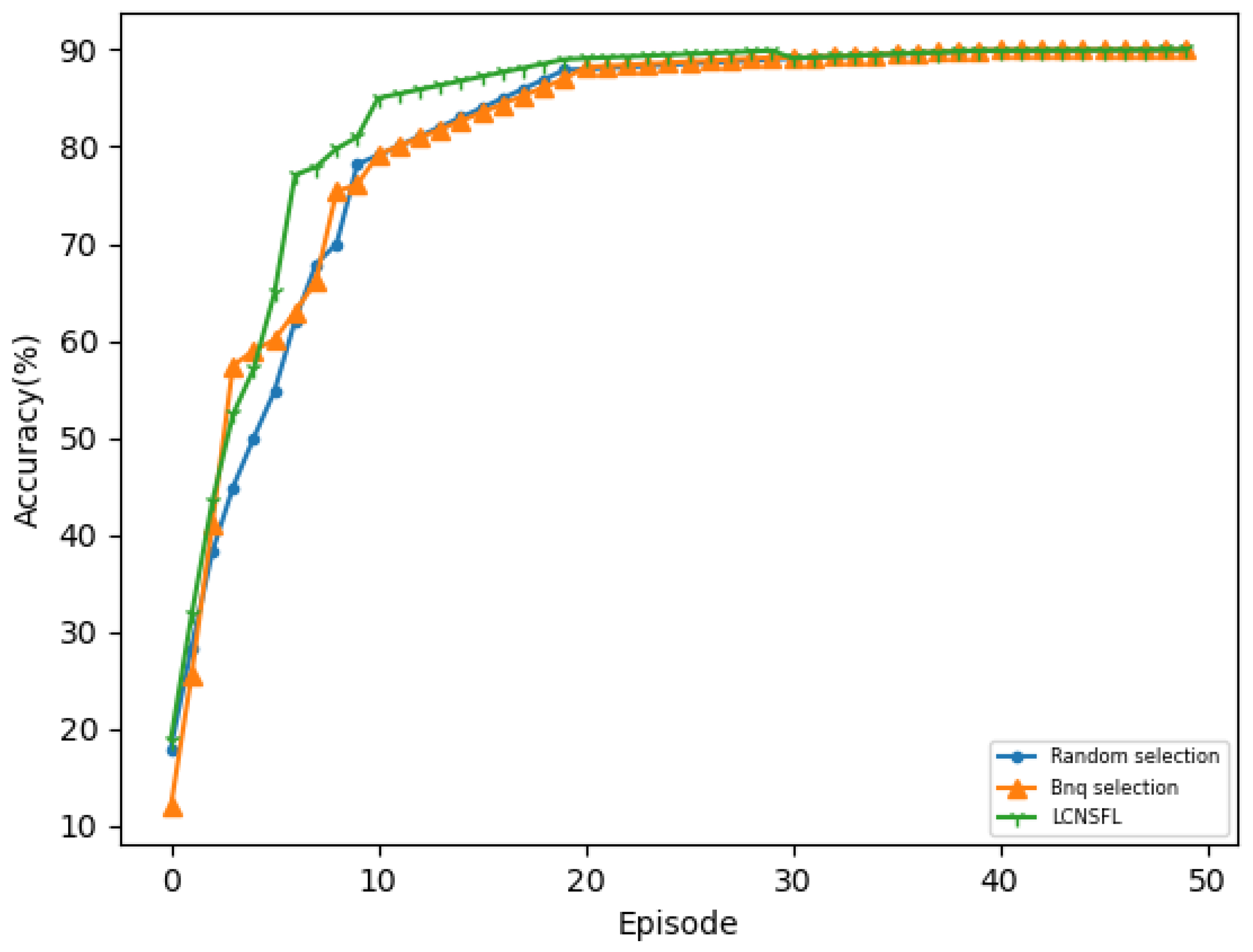
To further confirm the superiority of the LCNSFL algorithm, we compared it with traditional node selection strategies, namely, the random selection and Bnq selection approaches. The results indicate that the random selection algorithm tends to select devices with weaker computing capabilities, poorer channel quality, or higher energy consumption in federated learning. While Bnq selection performs better than random selection in these aspects, the LCNSFL algorithm outperforms both strategies overall. Therefore, the LCNSFL algorithm, without compromising the global model’s accuracy, effectively reduces the time and energy costs per round of federated training in dynamic network scenarios through precise node selection, demonstrating robustness.
Overall, the LCNSFL algorithm offers a promising solution for addressing challenges in federated learning within the SAGIN framework, showcasing its effectiveness and robustness in dynamic network environments.


