Article

The Variation Characteristics of Stratospheric Circulation under the Interdecadal Variability of Antarctic Total Column Ozone in Early Austral Spring

1
Key Laboratory of Meteorological Disaster, Ministry of Education (KLME)/Joint International Research Laboratory of Climate and Environment Change (ILCEC)/Collaborative Innovation Center on Forecast and Evaluation of Meteorological Disasters (CIC-FEMD), Nanjing University of Information Science & Technology, Nanjing 210044, China
2
Key Laboratory for Meteorological Disaster Monitoring and Early Warning and Risk Management of Characteristic Agriculture in Arid Regions, China Meteorological Administration, Yinchuan 750002, China
3
Ningxia Hui Autonomous Region Climate Center, Yinchuan 750002, China
*
Author to whom correspondence should be addressed.
Remote Sens. 2024, 16(4), 619; https://doi.org/10.3390/rs16040619
Submission received: 11 January 2024 / Revised: 4 February 2024 / Accepted: 5 February 2024 / Published: 7 February 2024

Abstract

:
Antarctic Total Column Ozone (TCO) gradually began to recover around 2000, and a large number of studies have pointed out that the recovery of the Antarctic TCO is most significant in the austral early spring (September). Based on the Bodeker Scientific Filled Total Column Ozone and ERA5 reanalysis dataset covering 1979–2019, the variation characteristics of the Antarctic TCO and stratospheric circulation for the TCO ‘depletion’ period (1979–1999) and the ‘recovery’ period (2000–2019) are analyzed in September. Results show that: (1) Stratospheric elements significantly related to the TCO have corresponding changes during the two eras. (2) The interannual variability of the TCO and the above-mentioned stratospheric circulation elements in the recovery period are stronger than those in the depletion period. (3) Compared with the depletion period, due to the stronger amplitude of the planetary wave 1, stronger Eliassen–Palm (EP) flux corresponds to EP flux convergence, larger negative eddy heat flux, and positive eddy momentum flux in the stratosphere during the recovery period. The polar temperature rises in the lower and middle stratosphere and the polar vortex weakens in the middle and upper stratosphere, accompanied by the diminished area of PSC. This contributes to the understanding of Antarctic ozone recovery.

1. Introduction

From the late 1970s to the early 1990s, the Total Column Ozone (TCO) decreased rapidly over Antarctica during the austral spring (September–November), forming the Antarctic ozone hole [1], which was mainly caused by the significant increase in ozone-depleting substances (ODSs) as a result of additional anthropogenic emissions of chlorofluorocarbons (CFCs) and bromocarbons [2]. Although ozone depletion will be exacerbated by the large amounts of volcanic aerosols produced by volcanic eruptions [3], ozone has been showing signs of healing since around 2000 [4,5,6,7], which is the year of peak ODSs [8,9]. Studies have shown that ozone recovery is most evident in September [10], and the signal of increasing ozone is strongest between 1 and 20 September due to the changes in ODSs [11]. As one of the reasons for ozone recovery in September, Solomon et al. [10] suggest that, on the one hand, it is the chemical impact that is attributed to the gradual reduction in halogenated gases due to the implementation of the Montreal Protocol. On the other hand, it is the dynamic impact due to the influence of stratospheric temperature and circulation.
The interdecadal trends of Antarctic ozone can be well explained by the changes in ODSs [12,13], while the interannual variation in ozone is mainly influenced by stratospheric temperature [14,15] and planetary waves [16,17,18]. When the Antarctic stratospheric temperature decreases to a certain temperature, Polar Stratospheric Clouds (PSC) begin to form and the area gradually increases, resulting in the heterogeneous chemical process of chlorine gas on the surface of these PSCs to destroy ozone [6]. Additionally, the cooling stratospheric temperature enhances the meridional temperature gradient from mid-latitude to polar regions, strengthens the polar vortex through the thermal wind balance [19], and delays the rupture time of the polar vortex [20]. Low-ozone concentration airs are restricted by the dynamic properties of a stronger and later burst of polar vortexes in the polar regions, providing material isolation for ozone hole development [21,22]. In addition, more upward or downward Eliassen–Palm (EP) flux, corresponding to the divergence of EP flux, propagates to the stratosphere and weakens the residual circulation and the ozone transport from mid-latitude to polar regions. The accompanying anomalous upward adiabatic cooling reduces the stratospheric temperature and enhances the polar vortex to eventually affect the ozone hole [23,24].
Antarctic ozone has an important impact on changes in the climate system. For example, the loss of Antarctic ozone cools the stratospheric polar region through radiation cooling and strengthens the circumpolar westerlies and polar vortex. The influence of Antarctic ozone depletion extends to the troposphere through complex interplays [25], enhances the southern annular mode, strengthens the westerly jet, shifts toward the pole, and deepens the Amundsen Sea lows. Moreover, the Hadley call and the subtropical arid zone move towards the polar region [26,27,28,29]. In addition, the existence of the Antarctic ozone hole also affects the ocean [30,31] and sea ice [32,33]. The climate effect of ozone recovery seems to be opposite to the climate change caused by ozone depletion [26,27,28,34]. In conclusion, there is a close but complex causal relationship between Antarctic ozone and stratospheric circulation. However, under the interdecadal change in TCO around 2000, the characteristics of stratospheric circulation anomalies and planetary waves are not well understood in the two preceding and following eras of the TCO ‘depletion’ period (1979–1999) and the ‘recovery’ period (2000–2019). Therefore, this paper plans to investigate the variation characteristics of stratospheric circulation and planetary waves during the two eras. The article is organized as follows. The data and methods are briefly described in Section 2. In Section 3, the variation characteristics of TCO, stratospheric temperature, polar vortex, and PSC area over Antarctica are studied by diagnosing the recovery period and the depletion period. The variation characteristics of planetary waves during the two eras are then discussed. Finally, the conclusion and discussion are given in Section 4.

2. Data and Methods

2.1. Data

The timeframe of all datasets is from 1979 to 2019.
The TCO dataset is provided by the Bodeker Scientific Filled Total Column Ozone (BS–TCO) Database V3.5.1, with a horizontal resolution of 1° × 1.25° [35].
Stratospheric temperature, geopotential height, and wind field are obtained from the European Center for Medium-Range Weather Forecasts (ECMWF) ERA5, with a horizontal resolution of 0.25° × 0.25° [36].
The indices used in this study are as follows:
(1)
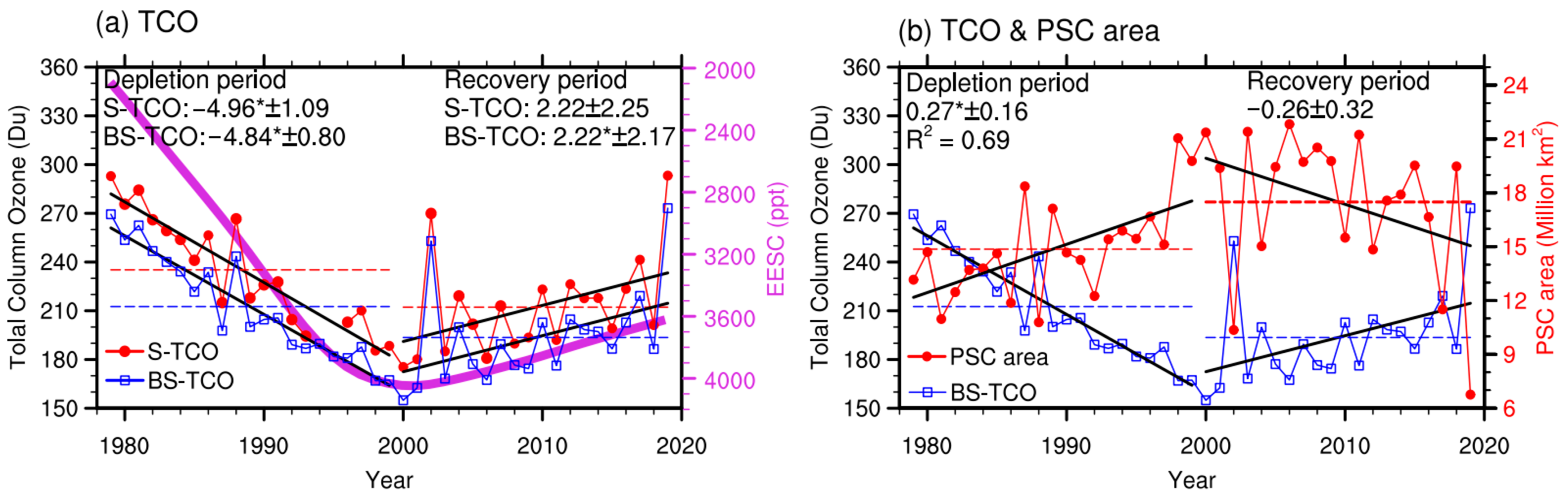
Polar TCO index from the BS–TCO dataset is TCO averaged over 63°S~90°S [10].
(2)
Polar TCO index from Satellite (S–TCO) is provided by the National Aeronautics and Space Administration (NASA) Goddard Space Flight Center online database, missing for 1994 and 1995.
(3)
Equivalent effective stratospheric chlorine (EESC) is obtained from the Goddard Space Flight Center, which has been widely used to relate predictions of human-generated ODS abundances to future ozone changes [5,12]. It uses the parameters suggested by Newman et al. [8,13] and corresponds to the WMO A1-2014 scenarios, with an age spectrum width of 2.75 year (symbol a is an abbreviation of year), a constant factor of 60, and a mean age-of-air of 5.5 a. This parameter is different from the classical EESC, which is thought to be more suitable for the polar region.
(4)
The index of the PSC area is also from the NASA Goddard Space Flight Center.
(5)
Due to the close correlation between TCO and polar (60°S~90°S) temperature, in particular with 50 hPa [12], the index of stratospheric temperature is represented by temperature averaged over 60°S~90°S (polar temperature, PT) at 50 hPa.
(6)
In the same way as the temperature, the polar vortex is greatly related to TCO, in which a 10 hPa polar vortex variability explains approximately 85% of the variance of polar TCO anomalies [37]. The index of the stratospheric polar vortex is also represented by geopotential height averaged over 60°S~90°S (polar geopotential height, PGH) at 10 hPa.
(7)
Additionally, the index of the stratospheric polar vortex is calculated by the zonal-mean zonal wind (U) at 60°S (U at 60°S, U60) and 30 hPa, which has the highest correlation with TCO and approaches the center of the mean position of the polar vortex in the mid-stratosphere. The polar vortex tends to enhance (weaken) the reduced (elevated) PGH and the accelerating (decelerating) U60.

2.2. Methods

With the methods of linear regression analysis, the tendency rate of the TCO, stratospheric temperature, polar vortex, and PSC area were analyzed in the two eras. Correlation analysis was used to explore the relationship between the TCO and stratospheric temperature, polar vortex, and PSC area. Additionally, all datasets were detrended to eliminate the correlation coefficient. Wavelet analysis was used to analyze the interannual variability of total Antarctic ozone and stratospheric elements [38]. The main dynamic processes are discussed by planetary wave, which is expressed by EP flux. EP flux has been widely used to diagnose the propagation of atmospheric fluctuations and wave–flow interaction [39,40]. The formulas for EP flux and its divergence are as follows in spherical p coordinates [41]:
F   =   ( F φ ,   F p ) = ( a cos φ ( v u ¯ ) ,   f a cos φ   ( v θ ¯ ) / θ ¯ p )
· F = 1 a cos φ φ ( F φ cos φ ) + p ( F p )
where F is EP flux, ∇·F is its divergence (EP div), u and v represent zonal and meridional wind, θ is the potential temperature, a is the radius of the Earth, f is the Coriolis parameter, φ is the latitude, p is the pressure (hPa), the overbars denote zonal averages, and the primes denote departure from the zonal average. v θ ¯ is the eddy heat flux (EHF). v u ¯ is the eddy momentum flux (EMF). EP flux convergence (divergence) will lead to the weakening (strengthening) of zonal flow. The EHF, being consistent with EP flux divergence [42], is related to the vertical component of EP flux [43] and reflects upward wave propagations [44]. The propagation of planetary waves can change EMF by adjusting the wave-driving rate of the polar vortex [39]. In the southern hemisphere, a negative EHF reflects upward wave propagation, while a positive EMF reflects the enhanced poleward motion [45]. Table 1 shows the abbreviations and full names of terms used in the text.

3. Results

3.1. The Variation Characteristics of Antarctic Total Column Ozone and Stratospheric Circulation during the Recovery Period and Depletion Period

Antarctic ozone is related to stratospheric temperature [14]. Stratospheric temperature affects the formation of PSCs on the one hand and cooperates with polar vortex on the other [6,22]. The Antarctic ozone experiences an interdecadal change characteristic of decreasing before 2000 and then rising after 2000 [7]. In consideration of that the variations in temperature, wind, and geopotential height are interrelated within the framework of a common physical process. So, do stratospheric temperature, polar vortex, and PSC area change correspondingly?

3.1.1. The Temporal Characteristics of Antarctic Total Column Ozone

Based on the BS–TCO, S–TCO, and EESC data, Figure 1a shows the time series of Antarctic polar TCO in September and EESC during the past 41 years (1979–2019). The polar TCO derived from different datasets shows consistent interannual variation and linear trend. The polar TCO coming from BS–TCO and S–TCO both increase at a rate of 22.2 Du·decade−1, with an average of 193.6 Du and 212.2 Du, respectively, in the recovery period. The trend from the BS–TCO dataset has passed the 0.05 significance test. The polar TCO coming from BS–TCO and S–TCO decreases significantly at a rate of 48.4 Du·decade−1 with an average of 212.6 Du and 49.6 Du·decade−1 with an average of 235.2 Du, respectively, in the depletion period. The trend and average are very different between the two periods. Following the phasing out of ODSs under the Montreal Protocol, the level of EESC stops rising before 2000 and decreases after 2000 in the polar stratosphere, corresponding to the depletion and recovery of TCO. The trend in the recovery period is numerically about twice as slow as the trend in the depletion period, partly due to the slow decreasing rate and long atmospheric lifetime of EESC, partly possibly due to short data records. Since the trend values obtained from the two datasets exhibit little difference and the S–TCO is incomplete, the BS–TCO dataset is used in the following analysis.
Antarctic ozone is directly related to the heterogeneous chemical process on the surface of PSC [6,46]. Figure 1b shows the time series of polar TCO and PSC area in the last 41 years. It can be seen that the PSC area is similar to the evolution of polar TCO and significantly related to polar TCO with a determination coefficient of about 0.7. The PSC area decreases slowly at a rate of 2.6 million·Km2·decade−1 with an average of 17.5 million·Km2 in the recovery period, corresponding to the increased polar TCO. The PSC area increases significantly at a rate of 2.7 million·Km2·decade−1 with an average of 14.9 million·Km2 in the depletion period, being consistent with the decreased polar TCO. Therefore, the PSC area first increases and then decreases around 2000.

3.1.2. The Temporal Characteristics of Stratospheric Temperature and Polar Vortex

The evolution characteristics of stratospheric temperature, geopotential height, and zonal wind have been analyzed in the recent 41 years. Figure 2 shows the time series of the polar TCO, 50 hPa PT, 10 hPa PGH, and 30 hPa U60 in the recent 41 years; 50 hPa PT, 10 hPa PGH, and 30 hPa U60 have a remarkable correlation with polar TCO with a determination coefficient of about 0.5. During the recovery period, 50 hPa PT and 10 hPa PGH increase at a rate of 1.8 K·decade−1 with an average of 195.5 K and 11.4 dagpm·decade−1 with an average of 2836.1 dagpm, respectively, while 30 hPa U60 decreases at a rate of 1.4 m·s−1·decade−1 with an average of 60.1 m·s−1. It can be seen that the trends of each stratospheric circulation element are not obvious, but correspond to the slow increase in TCO. During the depletion period, 50 hPa PT and 10 hPa PGH show a decreasing trend at a rate of 0.7 K·decade−1 with an average of 194.1 K and 6.1 dagpm·decade−1 with an average of 2825.3 dagpm, respectively, while 30 hPa U60 increases at a rate of 1.3 m·s−1·decade−1 with an average of 62.6 m·s−1. It shows that the cooling temperature, the reduced geopotential height, and the accelerating zonal wind correspond to the decreased polar TCO.
The above analysis results show that TCO and the temperature at 50 hPa, as well as the geopotential height at 10 hPa (PSC area and the zonal wind at 30 hPa), maintain a significant and stable positive (negative) relationship during the whole analysis period. In the depletion period, the stratospheric temperature decreases significantly, while the polar vortex increases significantly, and the zonal wind is stronger. At this time, the PSC area increases significantly, corresponding to the sharp decrease in TCO. In the recovery period, the higher stratospheric temperature, the weaker polar vortex, the smaller zonal wind, and the decreased PSC area, in which the trends are not obvious, agree with the slow increase in TCO.

3.1.3. The Spatial Characteristics of Antarctic Total Column Ozone and Stratospheric Circulation

To compare the spatial difference in TCO, stratospheric temperature, and polar vortex over Antarctica between the two eras, the composite of TCO and 50 hPa temperature anomalies, as well as 10 hPa geopotential height and 30 hPa zonal wind anomalies in comparison with the climatic mean state, are displayed in Figure 3 during the two periods. This indicates that significantly negative TCO anomalies are observed from Queen Maud Land to West Antarctica (cold shadings in Figure 3a) and the anomaly centers are located in the Haakon VII Sea (near 0°) during the recovery period. The positive TCO anomalies in Wilkes Land and its northern areas (warm shadings in Figure 3a) correspond to the positive anomaly center of the temperature (red contours in Figure 3a) and geopotential height (warm shadings in Figure 3c), as well as the anomalous eastward wind around 60°S (blue contours in Figure 3c). The distributions of TCO and stratospheric circulation anomalies during the depletion period are opposite to those during the recovery period Therefore, notable changes in TCO, stratospheric temperature, and polar vortex anomalies can be seen between the two periods. The positive (negative) TCO anomalies over Antarctica agree with the warming (cooling) of polar temperature and the weakening (strengthening) of the polar vortex.
Aiming at further understanding the linear trends of Antarctic TCO, stratospheric temperature, and polar vortex in the two eras, the spatial distributions of linear trends of TCO, 50 hPa temperature, 10 hPa geopotential height, and 30 hPa zonal wind are shown in Figure 4. During the recovery period, TCO (warm shadings in Figure 4a) and stratospheric temperature (red contours in Figure 4a) show a significant increasing trend over Antarctica, with the center located in the Ross Sea (near 180°). Geopotential height increases in the southern South Pacific (warm shadings in Figure 4c), accompanied by the decelerating zonal wind (blue contours in Figure 4c). During the depletion period, TCO (cold shadings in Figure 4b) and temperature (blue contours in Figure 4b) decrease significantly over Antarctica. Geopotential height decreases considerably over West Antarctica (cold shadings in Figure 4d) in combination with the accelerating zonal wind (red contours in Figure 4d).

3.1.4. The Interannual Variability of Antarctic Total Column Ozone and Stratospheric Circulation

The spatial characteristics of Antarctic TCO, stratospheric temperature, and polar vortex are significantly different between the recovery and depletion periods. For the purpose of contrasting the degree of interannual variation of the TCO and stratospheric circulation over Antarctica during the two periods, Figure 5 shows the composite variance of the TCO and 50 hPa temperature, as well as 10 hPa geopotential height and 30 hPa zonal wind during the two periods. As can be seen, the largest interannual variances of each element are located in Wilkes Land and its north during the recovery period (Figure 5a,c), and in the northeast of Queen Maude Land during the depletion period (Figure 5b,d). In addition, the interannual variance in the recovery period is greater than that in the depletion period and the center is consistent with that of the abnormal center on the whole (Figure 3). Therefore, the interannual variance distributions of TCO, stratospheric temperature, and polar vortex in the two periods are significantly different.
To further understand the interannual variability of Antarctic TCO and stratospheric circulation during the two periods, Figure 6 shows the Morlet wavelet analysis of polar TCO and 50 hPa PT during the two periods. As can be seen, the interannual variation in polar TCO and 50 hPa PT in the two periods is similar to the main cycle being 2–4 years. Lu et al. [47] and Zou and Gao [48] found that the Antarctic ozone has a quasi-biennial oscillation period, which is consistent with the results of this paper. In the 2–4 year cycle, the maximum power spectrum of the polar TCO was 1878 in the recovery period and 322 in the depletion period, while the maximum power spectrum of 50 hPa PT was 50 in the recovery period and 6.75 in the depletion period. The wavelet analysis of the PSC area, 10 hPa PGH, and 30 hPa U60 were similar to 50 hPa PT. Therefore, the power spectrum of the TCO and stratospheric circulation in the 2–4 year cycle during the recovery period are much greater than that during the depletion period, showing stronger interannual variability characteristics.
Combined with the above analysis results, it can be seen that the TCO is closely related to the PSC area, 50 hPa temperature, 10 hPa geopotential height, and 30 hPa zonal wind in the two eras. The relationship of each element is stable under the interdecadal change in the TCO: the rising (falling) of polar temperature, as well as the elevated (reduced) geopotential height, and the decelerating (accelerating) zonal wind result in the weakening (strengthening) of the polar vortex, combining with the increased (diminished) PSC area, thus, corresponding to the recovery (depletion) of the TCO. Additionally, the interannual variability of the TCO and stratospheric circulation in the recovery period is much greater than that in the depletion period.

3.2. The Variation Characteristics of Planetary Waves on Antarctic Total Column Ozone during the Recovery Period and Depletion Period

The above analyses prove that the 50 hPa temperature, 10 hPa geopotential height, and 30 hPa zonal wind are different during the recovery and depletion period. Are there also differences in the change in stratospheric circulation at each stratospheric layer between the two periods? First, the composite difference in stratospheric temperature, geopotential height, and zonal wind anomalies as a function of altitude and latitude were compared between the two periods. Compared with the depletion period, the temperature and geopotential height are positive anomalies in the polar region during the recovery period. The large value of temperature (geopotential height) is located in the lower and middle stratosphere (the middle and upper stratosphere). The zonal wind shows a negative anomaly near 60°S in the middle and upper stratosphere. Not only are the 50 hPa temperature, 10 hPa geopotential height, and 30 hPa zonal wind significantly different, but the temperature in the middle and lower stratosphere and the polar vortex in the middle and upper stratosphere are also significantly different between the two periods.
The linear trends of stratospheric temperature and polar vortex during the recovery and depletion periods are further analyzed. Figure 7 exhibits the linear trend of stratospheric temperature and geopotential height as a function of altitude and latitude in the two periods. It illustrates that the temperature shows a positive trend throughout the stratosphere and the maximum trends appear in the lower and middle stratosphere during the recovery period (Figure 7a). Additionally, the geopotential height shows a positive trend (Figure 7c), and the zonal wind shows a negative trend in the middle and upper stratosphere, indicating a rising temperature in the lower and middle stratosphere and the gradual weakening of the polar vortex in the middle and upper stratosphere. During the depletion period, the temperature shows a negative trend in the middle and lower stratosphere, and the maximum trend is in the middle stratosphere (Figure 7b), corresponding to the negative trend of geopotential height (Figure 7d) and the positive trend of zonal wind in the middle and upper stratosphere. This demonstrates the falling temperature in the lower and middle stratosphere and the strengthening polar vortex in the middle and upper stratosphere. The trends of stratospheric circulation are not obvious, consistent with the result from Figure 2. This is possibly because of its inhomogeneity in zonal distribution. As a consequence, the changes in temperature and polar vortex in the recovery period are opposite to that in the depletion period. The changes in temperature are mainly located in the middle and lower stratosphere, while the changes in polar vortex are in the middle and upper stratosphere.
The stratospheric temperature and polar vortex driven by planetary waves can affect the Antarctic ozone [23,24]. The difference in EP flux and EP flux divergence in the two periods are compared. The anomaly distribution in the recovery period is the opposite of that in the depletion period. In the recovery period, there is more upward EP flux and EP flux convergence in the stratosphere. The more downward EP flux corresponds to EP flux divergence during the depletion period, indicating the significant differences in EP flux and EP flux divergence between the two periods.
The linear trends of EP flux and EP flux divergence calculated from waves 1–3 as a function of altitude and latitude in the two periods are further displayed in Figure 8. During the recovery period, the stronger EP flux propagates from the troposphere to the stratosphere and EP flux convergence occurs in the middle and upper stratosphere above 10 hPa (cold shadings in Figure 8a). The stronger planetary wave forcings correspond to the positive trend of polar temperature in the lower and middle stratosphere and polar geopotential height in the middle and upper stratosphere (Figure 7a,c), as well as the negative trend of zonal flow in the middle and upper stratosphere being consistent with the recovery of the TCO. Additionally, in the vicinity of 3 hPa, EP flux is from the weak EP flux divergence in the low latitude (warm shadings in Figure 8a) to the EP flux convergence in the polar region. The stronger poleward movements are in favor of the transport of ozone-rich air from the equator to the polar, thus being consistent with the recovery of the TCO in the polar regions. In addition, the weak EP flux divergence exists near the polar region below 10 hPa (warm shadings in Figure 8a), which corresponds to the positive trend of zonal wind and the negative trend of geopotential height (cold shadings in Figure 7c). During the depletion period, the weaker EP flux exists from the troposphere to the stratosphere, corresponding to EP flux divergence at high latitudes in the middle stratosphere (warm shadings in Figure 8b). The weaker planetary wave forcings correspond to the negative trend of polar temperature in the lower and middle stratosphere and the polar geopotential height in the middle and upper stratosphere (Figure 7b,d). At this time, zonal flow accelerates in the middle and upper stratosphere, in favor of the depletion of the TCO. Additionally, EP flux is from EP flux divergence in the polar region to EP flux convergence in the low latitudes (cold shadings in Figure 8b). The weaker poleward movements are in favor of the transport of ozone from the polar to the equator, thus being consistent with the depletion of the TCO in the polar regions.
Eddy heat flux and eddy momentum flux can reflect the direction of planetary waves [40,45]. Figure 9 shows the difference in the linear trends of EHF and EMF calculated by waves 1–3 as a function of altitude and latitude between the two periods. During the recovery period, EHF decreases largely near the polar region of 10 hPa (Figure 9a), accompanied by more and stronger EP flux and EP flux convergence (Figure 8a). Compared with the recovery period, the smaller decreased EHF near the upper stratospheric polar region corresponds to weaker EP flux and EP flux divergence at high latitudes during the depletion period (Figure 8b). In addition, the increased EMF above 30 hPa at midlatitudes indicates that the poleward movements enhance (Figure 9b), and the planetary waves bring the ozone from the middle and low latitudes to the polar regions (Figure 8a), in keeping with the decelerating zonal flow and the increased ozone. During the depletion period, the decreased EMF in the stratosphere indicates that the poleward movements weaken and more planetary waves carry ozone away from the polar region (Figure 8b). This agrees with the accelerating zonal flow and the decreased ozone.
Planetary waves, particularly for wave 1, dominate the total wave in the stratosphere [42,49], Figure 10 shows the climatological distributions and composite anomalies for geopotential height calculated from wave 1, as well as the linear trends for geopotential height and temperature calculated from wave 1, at 100 hPa in September during the recovery period and depletion period. This demonstrates that positive geopotential height is observed from the east of the southern Indian Ocean to the center of the South Pacific (red contours in Figure 10a,b), while negative geopotential height is over the east of the South Pacific to the South Atlantic (blue contours in Figure 10a,b) during the two periods. During the recovery period, positive anomalies in the southeast Pacific (warm shadings in Figure 10a) and negative anomalies in the South Atlantic (cold shadings in Figure 10a) are superimposed with the climatological geopotential height, indicating the larger amplitude of geopotential height. From the perspective of the linear trend, the geopotential height wave 1 and temperature wave 1 are in different phases (Figure 10b), resulting in stronger baroclinic disturbance. During the depletion period, the anomalies for geopotential height are with out-of-phase superposition on the climatological geopotential height (Figure 10c). The geopotential height wave 1 and temperature wave 1 are in the same phases (Figure 10d), leading to weaker baroclinic disturbance.
In summary, the stronger (weaker) planetary wave amplitudes and baroclinic disturbances lead to stronger (weaker) upward planetary wave propagation from the troposphere to the stratosphere, as well as EP flux convergence (divergence), larger (smaller) negative EHF, and positive (negative) EMF. This is in accordance with the rising (falling) temperature in the lower and middle stratosphere and the weakened (enhanced) polar vortex in the middle and upper stratosphere, in combination with the diminished (increased) PSC area, being advantageous to the recovery (depletion) of the TCO.

4. Conclusions and Discussion

Based on the BS–TCO and ERA5 datasets during 1979–2019, this study explores the variation characteristics of TCO, stratospheric temperature, polar vortex, and PSC area over Antarctica under the interdecadal change in TCO around 2000 for the TCO ‘depletion’ period (1979–1999) and the ‘recovery’ period (2000–2019). The variation characteristics of planetary waves are then discussed during the two periods. The results are concluded as follows.
The TCO over Antarctica in September increases significantly after 2000 and decreases significantly before 2000 as a result of the change in ODSs. During the whole period, the TCO and the temperature, as well as the geopotential height (PSC area and the zonal wind) maintain a significant and stable positive (negative) relationship. Correspondingly, around 2000, the polar temperature in the middle and lower stratosphere experiences a process of first cooling and then warming, the polar vortex in the middle and upper stratosphere first strengthens and then weakens, and the PSC area first increases and then diminishes. The trends of stratospheric polar temperature and the polar vortex are not significant but are consistent with the changes in the TCO. However, the interannual variability of the TCO and the above-mentioned stratospheric circulation elements in the recovery period are stronger than in the depletion period. The complete picture of the variation characteristics of the TCO and stratospheric circulation during the recovery and depletion periods is presented in Figure 11.
During the recovery period (Figure 11a), due to the stronger amplitude of planetary wave 1 and the baroclinic disturbance in the upper troposphere (Figure 10a), stronger upward EP flux existed in the stratosphere, accompanied by EP flux convergence (Figure 8a), larger negative eddy heat flux, and positive eddy momentum flux (Figure 9) in the middle and upper stratosphere. The polar temperature rose (Figure 2a, Figure 4a and Figure 7a) in the lower and middle stratosphere and the polar vortex weakened (Figure 2b, Figure 4c and Figure 7c) in the middle and upper stratosphere. The area of PSC diminished (Figure 1b), in keeping with the recovery of the Antarctic TCO (Figure 1a and Figure 4a). During the depletion period (Figure 11b), the weaker planetary wave 1 amplitude and baroclinic disturbance in the upper troposphere (Figure 10c,d), resulted in weaker EP flux, together with EP flux divergence in the middle stratosphere (Figure 8b), smaller negative eddy heat flux and negative eddy momentum flux (Figure 9), when compared with the recovery period. The polar temperature fell (Figure 2a, Figure 4b and Figure 7b) in the middle and low stratosphere and the polar vortex was enhanced (Figure 2b, Figure 4d and Figure 7d) in the middle and upper stratosphere, accompanied by the increased area of PSC (Figure 1b), corresponding to the depletion of the Antarctic TCO (Figure 1a and Figure 4b).
The varying characteristics of the Antarctic ozone and stratospheric circulation are compared in this paper using monthly data from the past 41 years during the Antarctic TCO recovery period and depletion period. Stratospheric elements significantly related to the TCO experienced corresponding changes. The stronger interannual variability of the TCO and the stratospheric circulation elements possibly means that the dynamic processes of stratospheric circulation had a closer relationship with the TCO in the recovery period. But the time series of the TCO in Figure 1 and Figure 2 both have three local maximums in 1988, 2002, and 2019, because of sudden stratospheric warming [50,51]. Regarding the cause of the sudden stratospheric warming, some studies have suggested that it is due to the interaction between planetary waves and zonal winds [43], so this paper takes the three years of sudden stratospheric warming events into consideration as well. The results obtained after removing the data in these years are similar to those in this paper, so these three years do not affect the results presented in this paper. It is worth mentioning that the temporal and spatial characteristics of the Antarctic TCO from ECMWF are similar to those from BS–TCO. In addition, EP flux has a 2–4-year cycle and the power spectrum during the recovery period is much greater than that during the depletion period, showing stronger interannual variability characteristics. But the difference and interannual variability of EP flux are not significant between the two periods. Therefore, it is not analyzed deeply in this paper.
Due to the complex relationship between ozone and stratospheric temperature, and the continuous increase in greenhouse gases contributing to the cooling of the lower stratosphere in the depletion period and hindering the warming of the stratosphere in the recovery period [52], the order of precedence between TCO and stratospheric circulation is more difficult to distinguish. Solomon et al. [10] studied the contribution of dynamic and chemical processes to the ozone recovery trend through models and emphasized the important contribution of dynamic processes to ozone recovery in September. Additionally, an example of the relationship between stratospheric sudden warming and ozone studied for Syowa station in Antarctica based on the daily data, points out that stratospheric warming is affected by dynamic processes and ozone changes have a weak effect on stratospheric warming [53,54]. In conclusion, the formation of Antarctic ozone is influenced by atmospheric dynamics and atmospheric chemistry. It is necessary to select typical cases to analyze and further investigate the level of influence of dynamic processes on the TCO [55] using coupled dynamic chemical models in the recovery periods. In terms of the diagnosis of large-scale dynamic transport processes, a variety of diagnostic methods should be used for dynamic analysis, such as the residual circulation and reflective surfaces. Residual circulation driven by planetary wave activity [49] can also affect Antarctic ozone, but the long-term trends of this are still controversial [4,56]. All these problems need to be studied further.

Author Contributions

Conceptualization, methodology, J.L. and S.Z.; Writing—original draft, J.L.; Writing—review and editing, J.L. and M.W.; validation, D.G. and Y.Y.; funding acquisition, S.Z.; supervision, D.H. and Y.Y. All authors have read and agreed to the published version of the manuscript.

Funding

This work was funded by grants from the project of the National key research and development plan (Grant No. 2022YFF0801703), a key project of the National Natural Science Foundation (Grant No. 42030602), a major project of the National Natural Science Foundation of China (Grant No. 42192512), and an integration project of National Natural Science Foundation of China major research program (Grant No. 91837311).

Data Availability Statement

The dataset of the total ozone column is provided by Bodeker Scientific Filled Total Column Ozone (BS–TCO) Database V3.5.1 at https://doi.org/10.5281/zenodo.4535247 for this study (accessed on 1 October 2021). The polar ozone index from the satellite and the area of PSC formed of nitric acid trihydrate are from the National Aeronautics and Space Administration (NASA) Goddard Space Flight Center online database (https://ozonewatch.gsfc.nasa.gov/, accessed on 11 November 2021). The EESC dataset was obtained from https://acd-ext.gsfc.nasa.gov/Data_services/automailer/restricted/automailer (accessed on 27 November 2022). The stratospheric wind, geopotential height, and temperature datasets come from the European Center for Medium-Range Weather Forecasts (ECMWF) ERA5 at https://cds.climate.copernicus.eu/cdsapp#!/dataset/reanalysis-era5-pressure-levels-monthlymeans?tab=form (accessed on 14 December 2021).

Conflicts of Interest

The authors declare no conflicts of interest.

References

  1. Farman, J.C.; Gardiner, B.G.; Shanklin, J.D. Large losses of total ozone in Antarctica reveal seasonal ClOx/NOx interaction. Nature 1985, 315, 207–210. [Google Scholar] [CrossRef]
  2. World Meteorological Organization/United Nations Environment Programme (WMO/UNEP). Scientific Assessment of Ozone Depletion: 2014; Global Ozone Research and Monitoring Project Report No. 55; World Meteorological Organization/United Nations Environment Programme (WMO/UNEP): Geneva, Switzerland, 2014. [Google Scholar]
  3. Yu, P.; Davis, S.M.; Toon, O.B.; Portmann, R.W.; Bardeen, C.G.; Barnes, J.E.; Telg, H.; Maloney, C.; Rosenlof, K.H. Persistent stratospheric warming due to 2019–2020 Australian wildfire smoke. Geophys. Res. Lett. 2021, 48, e2021GL092609. [Google Scholar] [CrossRef]
  4. Hu, D.Z.; Guo, Y.P.; Wang, F.Y.; Xu, Q.; Li, Y.P.; Sang, W.J.; Wang, X.; Liu, M. Brewer-Dobson Circulation: Recent-Past and Near-Future Trends Simulated by Chemistry-Climate Models. Adv. Meteorol. 2017, 2017, 2913895. [Google Scholar] [CrossRef]
  5. World Meteorological Organization (WMO). Scientific Assessment of Ozone Depletion: 2018; Global Ozone Research and Monitoring Project-Report No. 58; World Meteorological Organization (WMO): Geneva, Switzerland, 2018; Volume 588. [Google Scholar]
  6. Hu, Y.-Y. The discovery of the Antarctic ozone hole. Chin. Sci. Bull. 2020, 65, 1797–1803. (In Chinese) [Google Scholar] [CrossRef]
  7. Stone, K.A.; Solomon, S.; Kinnison, D.E.; Mills, M.J. On recent large Antarctic ozone holes and ozone recovery metrics. Geophys. Res. Lett. 2021, 48, e2021GL095232. [Google Scholar] [CrossRef]
  8. Newman, P.A.; Daniel, J.S.; Waugh, D.W.; Nash, E.R. A new formulation of equivalent effective stratospheric chlorine (EESC). Atmos. Chem. Phys. 2007, 7, 4537–4552. [Google Scholar] [CrossRef]
  9. Chipperfield, M.P.; Bekki, S.; Dhomse, S.; Harris, N.R.P.; Hassler, B.; Hossaini, R.; Steinbrecht, W.; Thiéblemont, R.; Weber, M. Detecting recovery of the stratospheric ozone layer. Nature 2017, 549, 211–218. [Google Scholar] [CrossRef]
  10. Solomon, S.; Ivy, D.J.; Kinnison, D.; Mills, M.J.; Neely, R.R., III; Schmidt, A. Emergence of healing in the Antarctic ozone layer. Science 2016, 353, 269–274. [Google Scholar] [CrossRef]
  11. Strahan, S.E.; Douglass, A.R.; Damon, M.R. Why do Antarctic ozone recovery trends vary? J. Geophys. Res. Atmos. 2019, 124, 8837–8850. [Google Scholar] [CrossRef]
  12. Bian, L.G.; Lin, Z.; Zheng, X.D.; Ma, Y.F.; Lu, L.H. The trend of Antarctic ozone hole and its influencing factors. Adv. Clim. Chang. Res. 2012, 3, 68–75. [Google Scholar]
  13. Newman, P.A.; Nash, E.R.; Kawa, S.R.; Montzka, S.A.; Schauffler, S.M. When will the Antarctic ozone hole recover? Geophys. Res. Lett. 2006, 33, L12814. [Google Scholar] [CrossRef]
  14. Kravchenko, V.O.; Evtushevsky, O.M.; Grytsai, A.V.; Klekociuk, A.R.; Milinevsky, G.P.; Grytsai, Z.I. Quasi-stationary planetary waves in late winter Antarctic stratosphere temperature as a possible indicator of spring total ozone. Atmos. Chem. Phys. 2012, 12, 2865–2879. [Google Scholar] [CrossRef]
  15. Shantikumar, S.N.; Vemareddy, P.; Song, H.-J. Effect of lower stratospheric temperature on total ozone column (TOC) during the ozone depletion and recovery phases. Atmos. Res. 2020, 232, 104686. [Google Scholar]
  16. Chen, W.; Huang, R.H. The numerical Study of Seasonal and lnterannual Variabilities of Ozone due to Planetary Wave Transport in the Middle Atmosphere: Part I. The Case of Steady Mean Flows. Sci. Atmos. Sin. 1996, 20, 513–523. (In Chinese) [Google Scholar]
  17. Chen, W.; Huang, R.H. A Numerical Study of Seasonal and lnterannual Variabilities of Ozone due to Planetary Wave Transport in the Middle Atmosphere: Part II. The Case of Wave-Flow Interaction. Sci. Atmos. Sin. 1996, 20, 703–712. (In Chinese) [Google Scholar]
  18. Zheng, B.; Chen, Y.J.; Shi, C.H. Relationship of Zonal Ozone Seasonal Variations and Planetary Wave in the Stratosphere. Plateau Meteorol. 2006, 25, 366–374. (In Chinese) [Google Scholar]
  19. Thompson, D.W.J.; Solomon, S. Interpretation of recent Southern Hemisphere climate change. Science 2002, 296, 895–899. [Google Scholar] [CrossRef]
  20. Keeble, J.; Braesicke, P.; Abraham, N.L.; Roscoe, H.K.; Pyle, J.A. The impact of polar stratospheric ozone loss on Southern Hemisphere stratospheric circulation and climate. Atmos. Chem. Phys. 2014, 14, 13705–13717. [Google Scholar] [CrossRef]
  21. Waugh, D.W.; Plumb, R.A.; Elkins, J.W.; Fahey, D.W.; Boering, K.A.; Dutton, G.S.; Volk, C.M.; Keim, E.; Gao, R.-S.; Daube, B.C.; et al. Mixing of polar vortex air into middle latitudes as revealed by tracer-tracer scatter plots. J. Geophys. Res. 1997, 102, 13119–13134. [Google Scholar] [CrossRef]
  22. Zhang, Y.; Li, J.; Zhou, L.B. The Relationship between Polar Vortex and Ozone Depletion in the Antarctic Stratosphere during the Period 1979–2016. Adv. Meteorol. 2017, 2017, 3078079. [Google Scholar] [CrossRef]
  23. Li, C.C.; Guo, S.C.; Yi, Q.; Li, H.F. Relationship between atmospheric ozone and polar vortex intensity in the mid-high latitude over the Northern Hemisphere in winter. Plateau Meteorol. 2016, 35, 1290–1297. (In Chinese) [Google Scholar]
  24. Seidel, D.J.; Li, J.; Mears, C.; Moradi, I.; Nash, J.; Randel, W.J.; Saunders, R.; Thompson, D.W.J.; Zou, C.-Z. Stratospheric temperature changes during the satellite era. J. Geophys. Res. Atmos. 2016, 121, 664–681. [Google Scholar] [CrossRef]
  25. Kidston, J.; Scaife, A.; Hardiman, S.; Mitchell, D.; Butchart, N.; Baldwin, M.; Gray, L. Stratospheric influence on tropospheric jet streams, storm tracks and surface weather. Nat. Geosci. 2015, 8, 433–440. [Google Scholar] [CrossRef]
  26. Son, S.W.; Gerber, E.P.; Perlwitz, J.; Polvani, L.M.; Gillett, N.P.; Seo, K.-H.; Eyring, V.; Shepherd, T.G.; Waugh, D.; Akiyoshi, H.; et al. The impact of stratospheric ozone on Southern Hemisphere circulation changes: A multimodel assessment. J. Geophys. Res. 2010, 115, D00M07. [Google Scholar] [CrossRef]
  27. Polvani, L.M.; Waugh, D.W.; Correa, G.J.P.; Son, S.-W. Stratospheric ozone depletion: The main driver of twentieth-century atmospheric circulation changes in the Southern Hemisphere. J. Clim. 2011, 24, 795–812. [Google Scholar] [CrossRef]
  28. Banerjee, A.; Fyfe, J.C.; Polvani, L.M.; Waugh, D.; Chang, K.-L. A pause in Southern Hemisphere circulation trends due to the Montreal protocol. Nature 2020, 579, 544–548. [Google Scholar] [CrossRef]
  29. Zambri, B.; Solomon, S.; Thompson, D.W.J.; Fu, Q. Emergence of Southern Hemisphere stratospheric circulation changes in response to ozone recovery. Nat. Geosci. 2021, 14, 638–644. [Google Scholar] [CrossRef]
  30. Ferreira, D.; Marshall, J.; Bitz, C.M.; Solomon, S.; Plumb, A. Antarctic ocean and sea ice response to ozone depletion: A two-time-scale problem. J. Clim. 2015, 28, 1206–1226. [Google Scholar] [CrossRef]
  31. Seviour, W.J.M.; Gnanadesikan, A.; Waugh, D.W. The Transient Response of the Southern Ocean to Stratospheric Ozone Depletion. J. Clim. 2016, 29, 7383–7396. [Google Scholar] [CrossRef]
  32. Turner, J.; Comiso, J.C.; Marshall, G.J.; Lachlan-Cope, T.A.; Bracegirdle, T.; Maksym, T.; Meredith, M.P.; Wang, Z.; Orr, A. Non-annular atmospheric circulation change induced by stratospheric ozone depletion and its role in the recent increase of Antarctic sea ice extent. Geophys. Res. Lett. 2009, 36, L08502. [Google Scholar] [CrossRef]
  33. Zhang, J.K.; Tian, W.S.; Pyle, J.A.; Keeble, J.; Abraham, N.L.; Chipperfield, M.P.; Xie, F.; Yang, Q.H.; Mu, L.J.; Ren, H.-L.; et al. Responses of Arctic Sea Ice to Stratospheric Ozone Depletion. Sci. Bull. 2022, 67, 1182–1190. [Google Scholar] [CrossRef]
  34. Xia, Y.; Hu, Y.Y.; Liu, J.P.; Huang, Y.; Xie, F.; Lin, J.T. Stratospheric Ozone-induced Cloud Radiative Effects on Antarctic Sea Ice. Adv. Atmos. Sci. 2020, 37, 505–514. [Google Scholar] [CrossRef]
  35. Bodeker, G.E.; Kremser, S.; Tradowsky, J.S. BS Filled Total Column Ozone Database V3.5.1 (3.5.1). Zenodo 2021. [Google Scholar] [CrossRef]
  36. Hersbach, H.; Bell, B.; Berrisford, P.; Biavati, G.; Horányi, A.; Muñoz Sabater, J.; Nicolas, J.; Peubey, C.; Radu, R.; Rozum, I.; et al. ERA5 monthly averaged data on pressure levels from 1979 to present. Copernic. Clim. Chang. Serv. (C3S) Clim. Data Store (CDS) 2019, 10, 252–266. [Google Scholar]
  37. Seviour, W.J.M.; Hardiman, S.C.; Gray, L.J.; Butchart, N.; Maclachlan, C.; Scaife, A.A. Skillful Seasonal Prediction of the Southern Annular Mode and Antarctic Ozone. J. Clim. 2014, 27, 7462–7474. [Google Scholar] [CrossRef]
  38. Torrence, C.; Compo, G. A practical guide to wavelet analysis. Bull. Am. Meteorol. Soc. 1998, 79, 61–78. [Google Scholar] [CrossRef]
  39. Orr, A.; Bracegirdle, T.J.; Hoskings, J.S.; Jung, T.; Haigh, J.D.; Phillips, T.; Feng, W. Possible dynamical mechanisms for Southern Hemisphere climate change due to the ozone hole. J. Atmos. Sci. 2012, 69, 2917–2932. [Google Scholar] [CrossRef]
  40. Lubis, S.W.; Silverman, V.; Matthes, K.; Harnik, N.; Omrani, N.-E.; Wahl, S. How does downward planetary wave coupling affect polar stratospheric ozone in the Arctic winter stratosphere? Atmos. Chem. Phys. 2017, 17, 2437–2458. [Google Scholar] [CrossRef]
  41. Dunkerton, T.; Hsu, C.F.; McIntyre, M.E. Some Eulerian and Lagrangian Diagnostics for a Model Stratospheric Warming. J. Atmos. Sci. 1981, 38, 819–844. [Google Scholar] [CrossRef]
  42. Dunn-Sigouin, E.; Shaw, T.A. Comparing and contrasting extreme stratospheric events, including their coupling to the tropospheric circulation. J. Geophys. Res. 2015, 120, 1374–1390. [Google Scholar] [CrossRef]
  43. Song, B.-G.; Chun, H.-Y. Residual circulation and temperature changes during the evolution of stratospheric sudden warming revealed in MERRA. Atmos. Chem. Phys. 2016, preprint. [Google Scholar]
  44. Chemke, R.; Polvani, L.M. Linking midlatitudes eddy heat flux trends and polar amplification. NPJ Clim. Atmos. Sci. 2020, 3, 8. [Google Scholar] [CrossRef]
  45. Orr, A.; Lu, H.; Martineau, P.; Gerber, E.P.; Marshall, G.J.; Bracegirdle, T.J. Is our dynamical understanding of the circulation changes associated with the Antarctic ozone hole sensitive to the choice of reanalysis dataset? Atmos. Chem. Phys. 2021, 21, 7451–7472. [Google Scholar] [CrossRef]
  46. Huck, P.E.; McDonald, A.J.; Bodeker, G.E.; Struthers, H. Interannual variability in Antarctic ozone depletion controlled by planetary waves and polar temperature. Geophys. Res. Lett. 2005, 32, L13819. [Google Scholar] [CrossRef]
  47. Lu, L.H.; Bian, L.G.; Jia, P.Q. Short-term climatic change of Antarctic ozone. Q. J. Appl. Meteorol. 1997, 8, 402–412. (In Chinese) [Google Scholar]
  48. Zou, H.; Gao, Y.Q. QBO and ENSO Signals in Total Ozone over 60~70°S. Clim. Environ. Res. 1997, 1, 62–71. (In Chinese) [Google Scholar]
  49. Wang, Z.; Zhang, J.; Wang, T.; Feng, W.; Hu, Y.H.; Xu, X.R. Analysis of the Antarctic Ozone Hole in November. J. Clim. 2021, 34, 6513–6529. [Google Scholar] [CrossRef]
  50. Shen, X.C.; Wang, L.; Osprey, S. The Southern Hemisphere sudden stratospheric warming of September 2019. Sci. Bull. 2020, 65, 1800–1802. [Google Scholar] [CrossRef]
  51. Roy, R.; Kuttippurath, J.; Lefèvre, F.; Raj, S.; Kumar, P. The sudden stratospheric warming and chemical ozone loss in the Antarctic winter 2019: Comparison with the winters of 1988 and 2002. Theor. Appl. Climatol. 2022, 149, 119–130. [Google Scholar] [CrossRef]
  52. Maycock, A.C.; Randel, W.J.; Steiner, A.K.; Karpechko, A.Y.; Christy, J.; Saunders, R.; Thompson, D.W.J.; Zou, C.-Z.; Chrysanthou, A.; Abraham, N.L.; et al. Revisiting the mystery of recent stratospheric temperature trends. Geophys. Res. Lett. 2018, 45, 9919–9933. [Google Scholar] [CrossRef]
  53. Zou, H. Stratospheric sudden warming and its relationship with ozone on Antarctica in august. 1988. Antarct. Res. 1990, 2, 61–66. (In Chinese) [Google Scholar]
  54. Xiong, K.; Hu, R.M.; Shi, G.Y. Antarctic total ozone change correlated to the stratosphere wind and temperature during the polar night. Antarct. Res. 1992, 4, 45–50. (In Chinese) [Google Scholar]
  55. Shi, C.H.; Chen, Y.J.; Zheng, B.; Liu, Y. A comparison with the contribution of dynamics and chemistry in ozone’s seasonal variation in the stratosphere. Chin. J. Atmos. Sci. 2010, 34, 399–406. (In Chinese) [Google Scholar]
  56. Tian, W.S.; Huang, J.L.; Qie, K.; Wang, T.; Xu, M. Review of the general atmospheric circulation in the stratosphere and its variation features. J. Meteorol. Sci. 2020, 40, 628–638. (In Chinese) [Google Scholar]
Figure 1. Time series of (a) Antarctic polar TCO averaged over 63°S~90°S (dotted lines unit: Du) and EESC (purple line unit: ppt), as well as (b) polar TCO (blue square line) and PSC area (red dotted line, units: million·Km2) in September during 1979–2019. The left Y coordinate is for polar TCO. The right Y coordinate is for the inverse scale of EESC in (a) and for the PSC area in (b). The values on the top of the figure are linear trends in the recovery period (2000–2019) and depletion period (1979–1999). R2 in (b) is the determination coefficient for the whole period. * Indicates that the linear trends and correlation coefficients are significant at the 0.05 confidence level. The black lines are linear fits of the time series during the two periods. The dashed lines are the averages of the time series during the two periods.
Remotesensing 16 00619 g001
Figure 2. Same as Figure 1b, but for (a) 50 hPa PT averaged over 60°S~90°S (red dotted line, unit: K), (b) 10 hPa PGH averaged over 60°S~90°S (red dotted line, unit: dagpm), and (c) 30 hPa U60 (red dotted line, unit: m·s−1).
Remotesensing 16 00619 g002
Figure 3. Composite of (a,b) Antarctic TCO (shadings, unit: Du) and 50 hPa temperature (contours, unit: K), and (c,d) 10 hPa geopotential height (shadings, unit: dagpm), and 30 hPa zonal wind (contours, unit: m·s−1) anomalies in September during the (a,c) recovery period and (b,d) depletion period, in comparison with the climatic mean state. The climatic mean state is the average value of each element from 1980 to 2010. The dotted areas and yellow grid areas represent the anomalies in the (a,b) TCO and temperature, and (c,d) geopotential height and zonal wind that are statistically significant at the 0.1 confidence level, respectively. The outermost latitude is 30°S and the latitude interval is 15°.
Remotesensing 16 00619 g003
Figure 4. Same as Figure 3, but for the spatial distributions of the linear trends. The units of the trend of Total Column Ozone, 50 hPa temperature, 10 hPa geopotential height, and 30 hPa zonal wind are Du·a−1, K·a−1, dagpm·a−1, and m·s−1·a−1, respectively.
Remotesensing 16 00619 g004
Figure 5. Composite variances of (a,b) Antarctic Total Column Ozone (shadings, unit: Du2) and 50 hPa temperature (contours, unit: K2), and (c,d) 10 hPa geopotential height (shadings, unit: dagpm2) and 30 hPa zonal wind (contours, unit: m2·s−2) in September during the (a,c) recovery period and (b,d) depletion period.
Remotesensing 16 00619 g005
Figure 6. Morlet wavelet analysis of the (a,b) Antarctic polar TCO and (c,d) 50 hPa PT in September during the (a,c) recovery period and (b,d) depletion period. The black dots on the left represent passing the 0.05 confidence level and the power spectrum is on the right.
Remotesensing 16 00619 g006
Figure 7. The linear trends of (a,b) temperature (unit: K·a−1) and (c,d) geopotential height (unit: dagpm·a−1) as a function of altitude and latitude in September during the (a,c) recovery period and (b,d) depletion period. The dotted areas are significant at the 0.01 confidence level.
Remotesensing 16 00619 g007
Figure 8. The linear trends of EP flux (vectors, unit: m3·s−2·a−1) and EP flux divergence (shadings, unit: m·s−2·a−1) calculated from waves 1–3 as a function of altitude and latitude in September during the (a) recovery period and (b) depletion period. EP flux vectors are multiplied by the square root of 1000.0/p in both the vertical and horizontal directions, where p is pressure (hPa). Red vectors and dotted areas indicate that the EP flux and EP flux divergence are significant at the 0.05 confidence level according to Student’s t-test.
Remotesensing 16 00619 g008
Figure 9. Difference in the linear trends of (a) eddy heat flux (unit: K·m·s−1·a−1) and (b) eddy momentum flux (unit: m2·s−2·a−1) calculated from waves 1–3 as a function of altitude and latitude in September between the recovery period and depletion period.
Remotesensing 16 00619 g009
Figure 10. The (a,b) climatological distributions (contours) and composite anomalies (shadings) (unit: dagpm) for geopotential height calculated from wave 1 and (c,d) the linear trends for geopotential height (shadings, unit: dagpm·a−1) and temperature (contours, unit: K·a−1) calculated from wave 1 at 100 hPa in September during the (a,c) recovery period and (b,d) depletion period. Dotted areas are significant at the 0.05 confidence level according to Student’s t-test.
Remotesensing 16 00619 g010
Figure 11. Schematic diagram of the possible pathways for different evolutions of the Antarctic Total Column Ozone during the (a) recovery period and (b) depletion period.
Remotesensing 16 00619 g011
Table 1. Abbreviations and full names of terms used in the text.
AbbreviationsThe Full Name
TCOTotal Column Ozone
ODSsOzone-Depleting Substances
EESCEquivalent Effective Stratospheric Chlorine
PSC areaPolar Stratospheric Cloud Area
PTTemperature Averaged Over 60°S~90°S
PGHGeopotential Height Averaged Over 60°S~90°S
U60Zonal-Mean Zonal Wind (U) at 60°S
EMFEddy Momentum Flux
EHFEddy Heat Flux
Disclaimer/Publisher’s Note: The statements, opinions and data contained in all publications are solely those of the individual author(s) and contributor(s) and not of MDPI and/or the editor(s). MDPI and/or the editor(s) disclaim responsibility for any injury to people or property resulting from any ideas, methods, instructions or products referred to in the content.

