1. Introduction
Because of its beyond-the line-of-sight monitoring and all-weather-continuous remote sensing [
1,
2], high-frequency surface wave radar (HFSWR) has gained considerable attention. HFSWR has been widely used for two dominant areas: real-time maritime surveillance [
3] and sea surface target detection [
4,
5]. Among these, ship detection has been a focus of scholars and researchers [
6,
7]. The Range-Doppler (RD) image background contains various clutter mainly composed of sea clutter, ionospheric clutter, and dense targets’ interference [
8]. The existing research mainly focuses on continuously improving the target resolution ability.
The constant false alarm rate (CFAR) is a valuable point target detection technique based on comparing the neighboring reference cells’ mean energy [
9,
10]. This technique has been used in ship extraction by Hinz [
11] and Liu et al. [
12]. Dzvonkovskaya et al. [
13] analyzed the characteristics of sea clutter, meteor clutter, noise, and land reflection clutter and proposed an adaptive thresholding estimation strategy for HFSWR ship detection. In the case of two targets in the same cell, Rohling H [
14] proposed ordered statistical CFAR (OS-CFAR), which could effectively reduce the impact on the detection probability and the false alarm probability caused by inhomogeneous spatial distribution in local regions. Li et al. [
15,
16] improved the CFAR detector using spatial correlation as prior information. Experiments based on the CFAR detector have shown that spatial information is beneficial for improving the accuracy of dense targets detection.
Jangal et al. [
17] transformed the detection based on the spatial distribution characteristics of targets and clutter into image processing based on the morphology and distribution characteristics. They introduced the idea of wavelet-transform and proposed a target signal extraction method based on image decomposition. Researchers have combined the image processing technique with RD images of HFSWR and continuously improved them, achieving good results in target detection and clutter suppression. Baussard et al. [
18] analyzed the morphological features of the measured RD images and used curve analysis methods to remove components that interfere with target detection in the images. Subsequently, a ship detection technique based on the authentic RD images of HFSWR was proposed by Baussard et al. [
19], which exploits multi-scale variation and sparse representation morphological component analysis and obtains correct target detection results. Li et al. [
20] proposed a target detection method based on discrete wavelet transform (DWT), which automatically determines the optimal scale of wavelet transform instead of selecting based on experience.
Ocean surveillance using HFSWR is commonly performed in wide-range RD images. The targets to be detected in the RD images are very tiny. Regarding target detection, simple image processing methods rely on manual feature extraction and need more robustness. According to the existing HFSWR research, a two-stage intelligent processing algorithm is very suitable for the automatic extraction of an RD image’s optimal spatial features and performs well [
21,
22,
23]. In the first stage, many targets are quickly located, ensuring a high detection rate. In the second stage, false targets are removed. Existing research assumes that ships are independently distributed and treated as point targets. The information obtained in the study of isolated targets is limited. In HFSWR, the echoes from a single large-sized ship are concentrated in a single cell of the RD images and can be considered stable in a short period [
24]. Echo signals of ships sailing in a dense formation or group typically occupy multiple adjacent cells and present a specific spatial geometric shape. Peng et al. [
25] established a narrowband coherent radar multi-aircraft formation (MAF) echo model. They applied polynomial Fourier transform (PFT) to accurately identify the number of aircraft and the motion parameters of each aircraft. The experiments in a clean background have proven the effectiveness of the proposed method. Liang et al. [
26] simulated the over-the-horizon radar (OTHR) echo images of MAF with multipath effect using spectral color blocks number and amplitude. They adopted a convolutional neural network (CNN) to recognize the number of aircraft and conducted experiments in homogeneous clutter. In the complex background of HFSWR, research on formation detection and identification is limited.
In this paper, we propose a novel cascade identification algorithm for ship formation in the clutter edge. We first analyze the motion of HFSWR ship formation and establish a matching ship formation spatial distribution model. There are two types of formations with rigid structures that appear as extended targets with specific spatial shapes on the RD images. Then, we introduce the Faster R-CNN to locate the clutter regions and propose a two-stage formation identification algorithm. In the first stage, the extremum detector based on the gray value is employed to find cells with suspicious targets, and the Seed-Filling (SF) algorithm is introduced to connect multi-cell regions belonging to the same ship formation. An extremum detector based on connected regions is proposed to avoid duplicate detection of the same ship formation and reduce the data to be processed in the second stage. In the second stage, a lightweight CNN is designed to extract the convolutional features of suspicious targets. The highly abstract features extracted by CNN are input into the extreme learning machine (ELM) for efficient classification. We propose CNN-ELM to identify two densely distributed ship formations from inhomogeneous clutter and single-ship targets. The experimental results based on the factual HFSWR background demonstrate that our CNN-ELM model surpasses the classic Alexnet and Resnet18 in terms of the detection accuracy (97.5%) and processing time (0.871 s). Our proposed cascade identification algorithm performs excellently on datasets consisting of two types of ship formations and single-ship targets. Meanwhile, the proposed algorithm is tested on weak ship formation datasets (Weak set-1 and Weak set-2) and deformed formation datasets (Deformed set-1 and Deformed set-2). The proposed algorithm achieves an identification accuracy of 82% with an average signal-to-clutter ratio (SCR) of 5–7.5 dB. The proposed algorithm achieves an identification accuracy of 73.38% when the sub-targets deviate by 20% and an identification accuracy of 96.25% through transfer learning. Compared with the extremum detector combined with the classical CNN algorithm, our proposed algorithm performs excellently.
The rest of the paper is organized as follows. In
Section 2, we describe the spatial distribution model of ship formation. In
Section 3, we describe the proposed cascade identification algorithm. In
Section 4, we provide the experimental results and discussion. In
Section 5, we conclude.
2. Spatial Distribution Model of Ship Formation
Figure 1 shows the two-dimensional geometric model of several ship formations with multi-ships. The model discussed in this paper is universal and not limited to the following types. The ship formation movement observed by HFSWR can be analyzed from two perspectives: the formation center movement and sub-targets’ movement. The formation center is consistent with the overall ship formation movement, which has an absolute motion state. Sub-targets’ motion can be decomposed into absolute motion consistent with the ship formation motion, and relative motion relative to the formation center.
Referring to the inverse synthetic aperture radar (ISAR) imaging model [
27,
28], the relative motion of sub-targets can be abstracted as a rotational motion around the formation center.
Figure 2 shows the motion model of the ship formation. The HFSWR is located at the origin
O of the global coordinate system
XOY. The
X axis is tangent to the coast, and the
Y axis is perpendicular to the
X axis. The ships in formation are simplified as point targets, with one sub-target located at
. The formation center
is the reference point for measuring the position relationship of all sub-targets. The local coordinate system
xo′
y matches the distribution of ship formation, which is related to the control system of the formation. There is counterclockwise rotation at an angle of
from the global coordinate system
XOY to the local coordinate system
. The coordinate of sub-target
in the local coordinate system
is (
x,
y). The radar line of sight (RLOS) coordinate system
takes
as the coordinate origin, where the
r axis is consistent with the RLOS direction. The azimuth angle of the formation center
relative to the HFSWR varies between 0° and 180°. The ship formation with a constant velocity
sails along the
X axis direction of the global coordinate system. Their slowly changing heading can be assumed to be stable during the coherent integration time (CIT).
At time
, the distance from the sub-target
to the HFSWR can be expressed as:
where
is the distance between the formation center
and the radar at time
t1, and
is the azimuth angle of the
relative to the radar at time
t1. During the beyond-the line-of-sight monitoring of HFSWR, the absolute coordinate value of
is much smaller than
. The
can be approximated as:
At time
, where
is the time interval, the azimuth angle of
relative to the radar can be expressed as:
where
is the azimuth change during the time
,
, and
. Usually,
and
are very small. At time
t2, the distance between
and the radar can be approximated as:
where
is the coordinate of
in the
coordinate system, and it can be expressed as:
is the distance between
and the radar at time
t2, and
is the radial velocity of
relative to the radar.
The distance between the sub-targets and the HFSWR can be obtained through iteration during the CIT. The transmission waveform of HFSWR is a frequency-modulated interrupted continuous wave (FMICW). Assuming
t1 =
jTc is the end time of the
jth sweep, where
Tc is the sweep width, the (
j + 1)th sweep time can be represented by
where
q is the pulse period, and
T0 is the pulse width in seconds. The transmission waveform can be expressed as:
where
A is the amplitude of transmission signal,
fc is the carrier frequency, and
B is the bandwidth. The mixing output signal of the sub-target
can be expressed as:
where
C is the amplitude of the echo signal. The phase of the echo signal can be expressed as:
where the first item
is related to the distance between the formation center and the radar, and the second item
is related to the coordinate of
in the
coordinate system. The echo signal of the ship formation can be expressed as:
where
N is the number of sub-targets in the formations. The main influencing factors of amplitude
C include the transmission power, radar cross section (RCS), and distance. The echo amplitude of sub-targets is considered to be the same constant. The signal model is related to sub-target distribution and the ship formation motion.
During the CIT, the ship formation spatial distribution model is obtained by imaging the echo signal of multiple sweeps.
3. Proposed Cascade Identification Algorithm
In this section, we introduce the proposed cascade identification algorithm, which detects and identifies ship formations sparsely injected into the real clutter edges.
3.1. Cascade Identification Algorithm Framework and Preprocessing
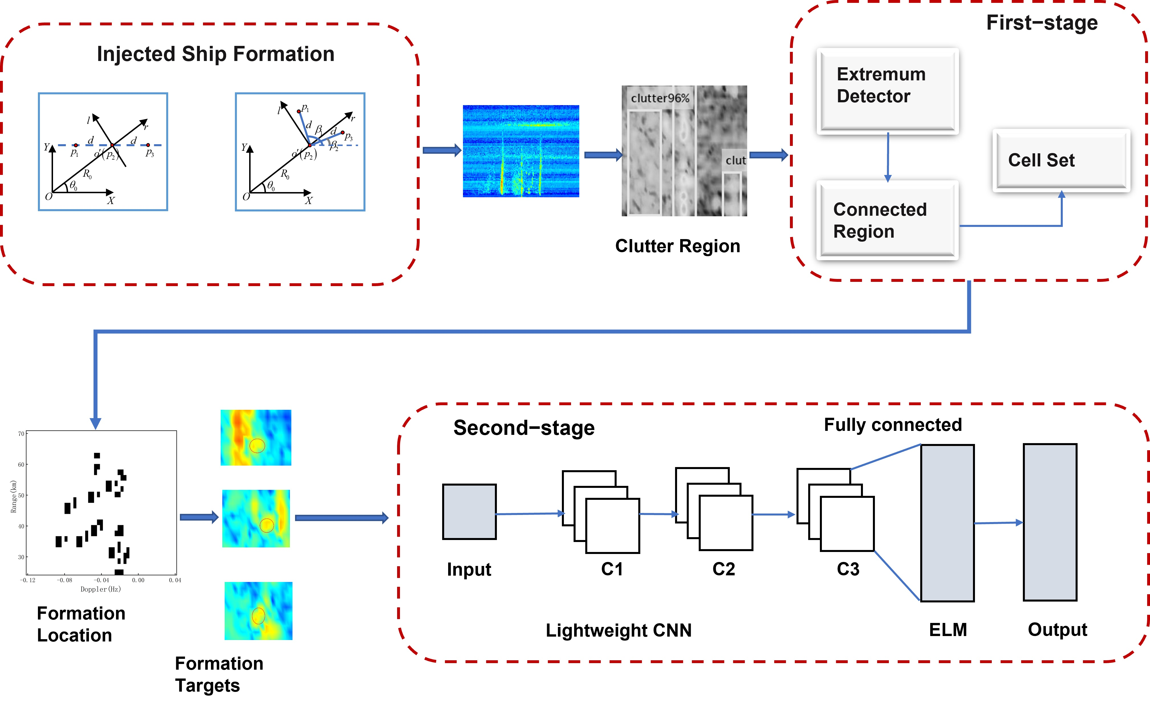
Figure 3 shows the framework of the proposed algorithm. In the preprocessing stage, the Faster R-CNN is introduced to locate the clutter region of the collected RD images. In the first stage, an extremum detector based on connected regions is proposed to extract targets. The processing principle in this stage is to avoid losing targets, quickly obtain all suspicious targets, and group the ship formation for output. In the second stage, a CNN-ELM is designed to eliminate false targets and identify two densely distributed ship formations.
Compared to color images, grayscale images are less space-consuming and retain essential information, which is suitable for real-time processing. Before the preprocessing stage, the color RD images are transformed into grayscale images, and the grayscale value of each pixel can be expressed as
where
,
, and
are the weights of
,
, and
, respectively.
In the preprocessing stage, Faster R-CNN is merely used to distinguish the clutter regions and locate them. Faster R-CNN is a target classifier in multi-region-based proposals [
29], and attention-oriented Region Proposal Networks (RPN) extract the interest regions. Using convolutional image feature maps shared with RPN, the fully connected layer can adopt a deep network and improve the quality of proposals.
The default feature extraction and target classification network of the Faster R-CNN is the VGG-16. The VGG-16 consists of 5 convolutional layers and 13 shared layers, suitable for large-volume datasets with over 10
4 images. The dataset composed of images mentioned in
Section 4.2 cannot meet the training requirements of VGG-16. We replaced the original VGG-16 with Resnet50. The Resnet50 introduces residual modules to avoid the problems of gradient vanishing and model degradation.
3.2. Extremum Detector Based on Connected Region
The grayscale values of target and sea clutter are lower than in the background. Ship formation occupies more stable high-energy cells than the single-ship target, which appears as an isolated point. In this stage, an extremum detector based on connected regions is adopted.
First, the discrimination criteria for the extremum detector are expressed as:
where
is the threshold factor,
k0 is the average grayscale value of the reference cells, and
h(xtest) is the grayscale value of the tested cell
xtest. 1 indicates the cell is a suspicious target, and 0 indicates the background. We adjust the threshold factor
to ensure the extremum detector detects all targets.
Then, the SF algorithm is introduced to connect the cells with suspicious targets. The cells with are seeds, of which the grayscale value is set to 0. We traverse the four adjacent cells around the seeds, including the top, bottom, left, and right, and merge the cells with the grayscale value of the 0 value into a connected region. We search for connected regions using the newly merged cells as seeds. The detection process will continue until all the cells with suspicious targets have been traversed.
3.3. Lightweight CNN-ELM
CNN performs well in extracting image features and identifying real targets contaminated with clutter [
21]. ELM is a feedforward network with a single hidden layer, which has a simple and effective training method and can quickly obtain local optimal solutions. We design a CNN-ELM classifier to identify ship formations in the clutter edge. The structure of the lightweight CNN is based on Alexnet and was determined after extensive debugging. To accelerate the network speed, the designed CNN is shallower than Alexnet. The lightweight CNN consists of three convolution layers, two pooling layers, and two fully connected layers. A dropout layer was added to the third convolution layer to prevent overfitting. The network structure is given in
Table 1. Compared to Alexnet, the proposed lightweight CNN has fewer pre-training parameters.
4. Experiment and Discussion
In order to demonstrate the effectiveness of the proposed cascade identification algorithm, experiments are conducted using simulated targets and measured RD image backgrounds. We present the experimental parameters including the measured background and different types of formations, in
Section 4.1. The RD data structure and multiple datasets are introduced in
Section 4.2. The model training and formation identification are presented in
Section 4.3. We also evaluate the performance of the proposed algorithm in the case of weak and deformed formation identification in
Section 4.4.
4.1. Experiment Parameters
The origin RD data, composed of various clutter and targets, are obtained through the HFSWR system located in the city of Weihai. The HFSWR system parameters are given in
Table 2. The real targets are artificially removed from the measured data, and simulated targets, including two types of ship formations shown in
Figure 4 and single-ship targets, are injected into the clutter edge position of RD images.
The geometric parameters of the single-column formation and the V-shaped formation are shown in
Table 3.
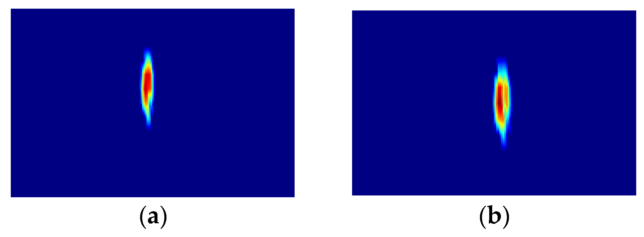
Figure 5 shows the spatial distribution model of the two formations without clutter.
Figure 6 shows the distribution of the single-column and V-shaped formation in the RD images. The constructed RD images cover widely in the range and Doppler domains. The images have been cropped for ease of display in
Figure 5 and
Figure 6. The two types of ship formations have the same parameters, except for the formation shape. For the single-column formation, the maximum difference between the sub-targets and the formation center in the range and Doppler domains is 1.03 km and 0.0022 Hz, respectively. For the V-shaped formation, the maximum distance of the sub-targets and formation center in the range domain is 1.75 km, and the gap between
and
in the Doppler domain is 0.0019 Hz. There is less difference between sub-targets in the range domain and Doppler domain than in the HFSWR resolution given in
Table 2. Formations are presented as extended targets with slight differences in outline.
We also analyze the distribution feature of the weak formation and deformed formation.
The target energy is measured by the SCR, and the SCR is expressed as:
where
is the amplitude of the target center, and
is the average amplitude of the reference clutter.
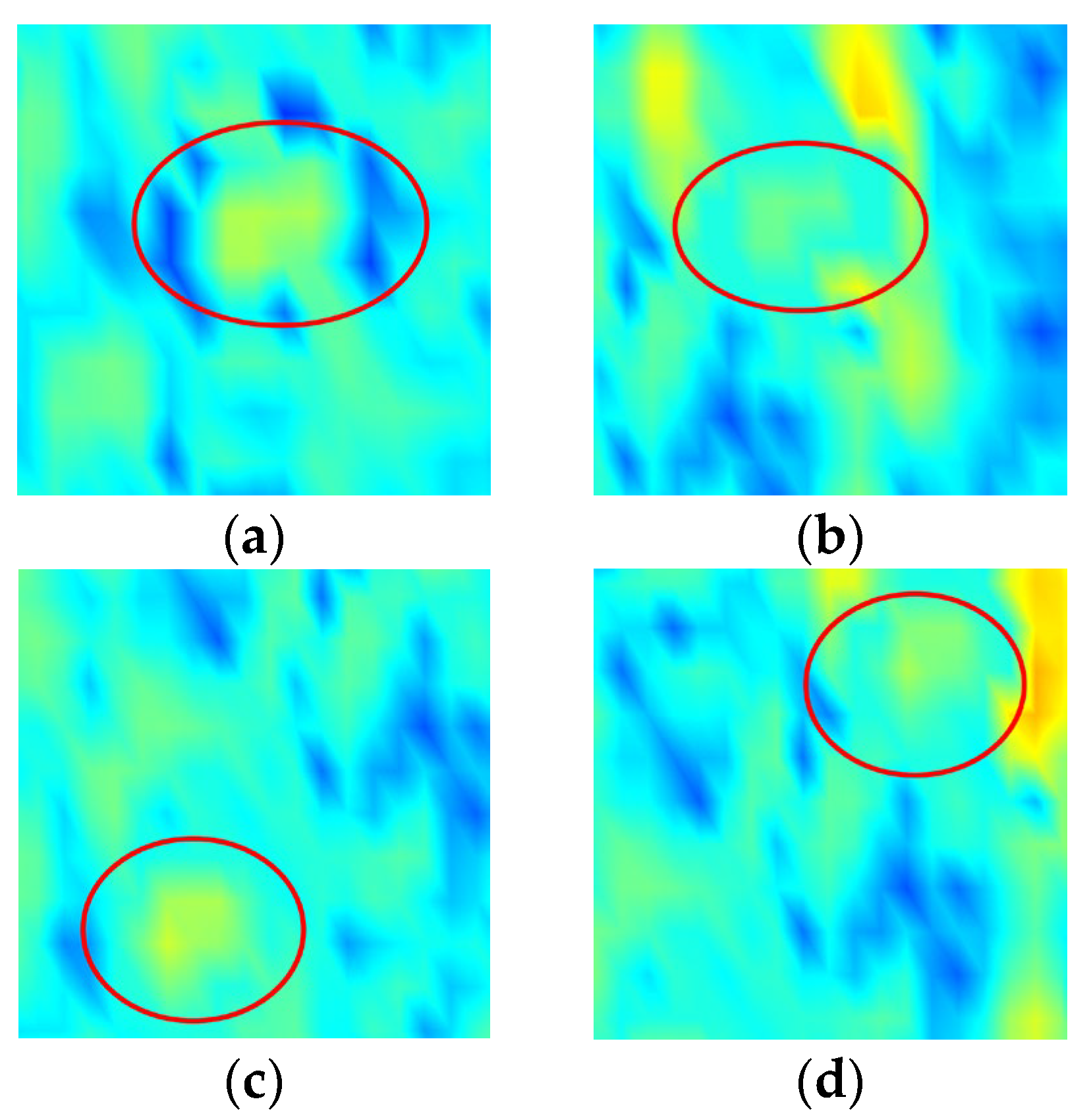
Figure 7 shows ship formations with low SCR. Moreover, the ship formations with SCR of 5 and 7.5 dB almost blend into the background.
Figure 8 shows the deformed formation. Based on the original values, the distance between the formation center and the sub-targets is increased by 5% and 20%. Ship formations change very little at the deviation of 5%. At the deviation of 20%, the single-column formation is stretched, and the sub-targets of the V-shaped formation can be distinguished.
4.2. Data Structure and Dataset
The size of the RD images constructed in
Section 4.1 is 4480 × 300 pixels. The color RD images are transformed into grayscale images and fed into the pre-trained Faster R-CNN to extract clutter regions. The extremum detector processes the clutter region images captured from the RD images. The first stage output consists of multiple connected regions, each represented by a set of cells from the same ship formation or a single-ship target. In the second stage, a fixed-size 2D sliding window is selected to capture target data from the images, with the center of the sliding window located at the center of the connected regions. Considering the size criteria of the window in detectors [
15,
16] and the characteristics of our data, the range and Doppler direction of the sliding window are set to 20 cells. The output of the CNN-ELM classifier is the identification results.
The preprocessing stage focuses on quickly extracting clutter regions rather than a profound study on the Faster R-CNN algorithm. We create a Faster R-CNN dataset containing 20 RD images and label the sea clutter. In the first stage, 20 RD images are selected as test samples, each with 45 targets at the edge of the clutter. The sample set is used to determine the threshold factor of the extremum detector. In the second stage, the dataset consists of equal proportional single-ship targets, single-column formations, V-shaped formations, and backgrounds. The SCR of the targets ranges from 5 dB to 25 dB. The dataset contains 4000 images and is randomly split into three parts: three-fifths of which is used as a training set, one-fifth of which is used as a validation set, and one-fifth of which is used as a testing set.
We also construct datasets for the weak and deformed formation identification separately. Each dataset contains 20 RD images, each with 45 targets at the edge of the clutter. The proportion of single-ship targets, single-column formations, and V-shaped formations is consistent. In the “Weak set-1” and “Weak set-2”, the SCR of the targets is 7.5 to 10 dB and 5 to 7.5 dB, respectively. In the “Deformed set-1” and “Deformed set-2”, the sub-targets are deviated by 5% and 20%, respectively.
4.3. Experimental Results
Faster R-CNN is pre-trained on ImageNet. According to the size of the clutter regions in multiple RD images, the anchors of the Faster R-CNN are adjusted to three scales (642,1282, and 2582 pixels) and three aspect ratios (0.5, 1.0, and 2.0). The anchors match the real target box with an overlap of more than 0.5.
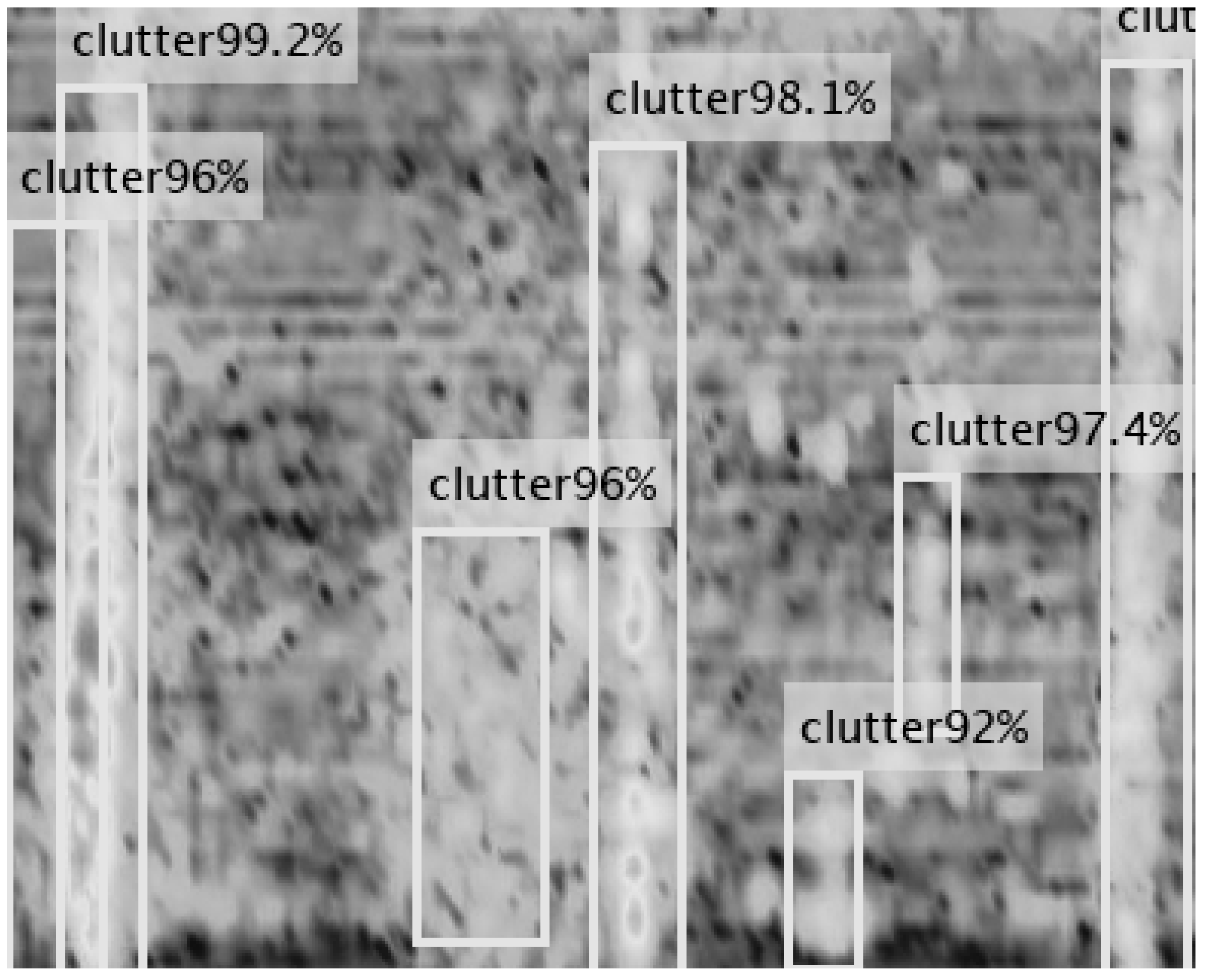
Figure 9 shows the clutter detection results of the Faster R-CNN. The bright vertical bar regions in the images are identified as sea clutter regions. The scores on the top indicate that the network has good recognition performance for sea clutter and meets the requirements of the preprocessing stage.
Figure 10 shows the grayscale distribution of single-ship target and single-column formation. The closer the cell is to the center regions, the lower the grayscale value and the higher the energy. Ship formation occupies more stable high-energy cells than the single-ship target, which appears as an isolated point.
The threshold factor
is experimentally determined to be 0.9, and the extremum detector can detect all targets.
Figure 11 shows an example of the target detection results, and the connected regions shown in black contain potential targets. From the detection results, targets are hit without any omissions. Taking
Figure 11 as an example, the output of a pure extremum detector is separate cells with a quantity of 65, and the output of the connected region extremum detector is cell sets with an amount of 23. The two types of extremum detectors obtain the same cells but different output forms. The pure extremum detector extracts RD region images with 65 separate cells as the image center. In contrast, the extremum detector proposed extracts images with the cell set center as the image center. The RD region images to be classified in the second stage are reduced by 182.61% using the proposed first stage detector. From the above analysis, we have concluded that the proposed extremum detector can improve the efficiency of the cascade identification algorithm.
We train the CNN-ELM step by step, and the process is as follows:
Train the lightweight CNN using labeled datasets, and adjust the parameters until the training accuracy reaches 80%;
Replace the output layer of the CNN with the ELM, and train the ELM using highly abstract features extracted by the CNN until the expected results are achieved;
Obtain a hybrid CNN-ELM model.
Based on the features of the input and empirical data, the parameters, including the initial learning rate and batch size, are adjusted to minimize training losses. The batch size of 128 and initial learning rate of 0.001 are finally applied to the CNN-ELM model, considering the training effectiveness and the running time.
The proposed CNN-ELM is compared with the classical Alexnet and the Resnet18 used in [
26]. The Alexnet consists of five convolution layers and three fully connected layers, with activation functions for ReLU and Dropout layers to enhance the model generalization ability. The Resnet18 has a shallow depth and contains four stacked residual blocks. Precision, recall, accuracy, and processing time are used as the network evaluation metrics. The precision and recall can be expressed as:
where
is the number of true targets detected,
is the number of true targets missed, and
is the number of false targets detected. The multi-category problem is transformed into a binary classification problem, where the precision and recall of each category are calculated separately. The accuracy is expressed as the ratio of the number of correctly classified samples to the total number of samples, used to describe the global accuracy of the model. The processing time refers to the average processing time of each image, expressed as the ratio of the testing set processing time to the number of test samples.
Table 4 shows the performances of the three networks.
Table 4 shows that the three networks can distinguish single-ship targets, two types of dense ship formations, and backgrounds, with a classification accuracy of over 90%. From the first seven rows of
Table 4, both our proposed network and Alexnet are on the level of precision and recall parameters and are superior to Resnet18. In addition, the proposed network achieves a slightly better performance in accuracy than Alexnet. The reason is that the lightweight CNN met the feature extraction requirements of the target morphology and energy, and the ELM improved the generalization ability and noise resistance. Regarding training and processing time, our proposed network is significantly better than Alexnet and Resnet18. This is due to the CNN-ELM having a shallower network structure. In summary, the designed CNN-ELM performs well.
We compare the proposed cascade identification algorithm with the extremum detector−Alexnet and extremum detector−ResNet18. The targets and identification results are annotated in the RD images. In
Figure 12, the single-ship targets are marked by boxes, circles mark the single-column formations, and triangles mark the V-shaped formations. The results indicate that the proposed algorithm can correctly identify ship formations and single-ship targets contaminated with clutter. The extremum detector−Alexnet and extremum detector−Resnet18 could only identify part of the targets.
4.4. Weak Formation and Deformed Formation Identification Results
Table 5 and
Table 6 show the accuracy of the proposed cascade identification algorithm, extremum detector−Alexnet, and extremum detector−Resnet18. The average accuracy of the targets with SCR of 5 and 7.5 dB is around 78%. In the case of deficient target energy, deep learning networks can still extract local spatial features. The proposed algorithm achieves better accuracy than others on the same dataset. The accuracy of the three algorithms slightly decreases at the deviation of 5%. At the deviation of 20%, the shape and energy changes in the target regions cause interference with the deep learning networks, and the accuracy of the three algorithms is greatly reduced.
The networks of the three algorithms are improved to meet the needs of deformable formation identification. The transfer learning can overcome the dependence on data and borrow generic features from pre-trained models for the target task [
30,
31]. The shallow layers of the CNN tend to extract generic features in the source domain, which could be transferred into the target domain. The features extracted by deep layers have specificity and cannot be transferred. The layer-by-layer freezing method is introduced to improve the training efficiency and robustness of the model by adjusting only the deep layer parameters. The training process is as follows:
Label the trained CNN-ELM model as S-model;
Freeze the first layer parameters of the S-model, adjust the parameters of the rest layers to achieve good performance for the target task, and label the trained CNN-ELM model as S-model1;
Freeze the first two layers with fixed parameters of the S-model, retrain, and label the model as T-model2;
Freeze the CNN parameters in the S-model, retrain the ELM, and label the model as T-model3;
Compare T-model1, T-model2, and T-model3, and determine the model with the best performance as the transfer learning model.
The datasets “Deformed set-1” and “Deformed set-2” are split into three parts, respectively, three-twentieths of which is used as a training set, one-twentieth of which is used as a validation set, and four-fifths of which is used as a testing set.
Table 7 shows the three algorithm identification results after transfer learning. The accuracy of each model has been improved. The CNN-ELM transfer learning model on the same dataset is better than Alexnet and Resnet18 in identification accuracy.
5. Conclusions
In this paper, we first investigate the spatial distribution model of ship formation for high-frequency surface wave radar (HFSWR) and propose a novel cascade identification algorithm for ship formation in the clutter edge. Taking single-column and V-shaped formations as examples, we analyze the distribution feature of the normal formation, weak formation, and deformed formation. Then, we introduce the Faster R-CNN to locate the clutter regions and propose a two-stage formation identification algorithm. In the first stage, an extremum detector based on connected regions is employed to achieve rapid detection. The proposed extremum detector reduces the number of images classified in the second stage, improving the cascade algorithm’s efficiency. In the second stage, the CNN-ELM is proposed to classify the targets. Compared with the classical Alexnet and Resnet18, the proposed CNN-ELM can deal with the impact of clutter and single-ship targets well and obtain higher identification accuracy with lower computation and memory. Meanwhile, the experimental results based on the factual HFSWR background demonstrate that the proposed cascade identification algorithm is superior to the extremum detector combined with the classical CNN algorithm for ship formation identification. The proposed algorithm achieves an identification accuracy of 82% with an average signal-to-clutter ratio (SCR) of 5–7.5 dB. At the deviation of 20%, our proposed algorithm achieves an identification accuracy of 96.25% with limited samples through transfer learning. The future work will mainly focus on tracking and positioning of ship formation.


