Development of a Dynamic Prediction Model for Underground Coal-Mining-Induced Ground Subsidence Based on the Hook Function

Abstract

Underground coal-mining-induced ground subsidence deformation is a common geological disaster impacting buildings, transportation and water supplies. Models predicting ground subsidence dynamically with high precision are important for the prevention of damage derived from ground subsidence. In this paper, the Hook function is utilized to develop a model describing the velocity of ground subsidence due to underground coal mining. Based on the subsidence velocity model, a dynamic subsidence model is established by taking an integral of the velocity model. Coefficients of the model, which depend on maximum subsidence, maximum subsidence velocity and the time corresponding to the maximum subsidence velocity, are related to the geological and mining conditions of the coal seam being investigated. A Levenberg–Marquardt-algorithm-based method is also proposed to calculate the optimal model coefficients based on subsidence velocity observations. Four continuously operating Global Navigation Satellite System (GNSS) stations were constructed above a typical longwall coal mining working face in the Jining mining area, China. These GNSS stations collected subsidence observations over two years, which were used to validate the developed prediction model. The results show that the root-mean-square (RMS) of the model-predicted ground subsidence error is 56.1 mm, and the maximum relative error is 2.5% for all four GNSS stations, when the ground subsidence is less than 6000 mm.

1. Introduction

Coal is a major source of energy in the production of electrical power, currently providing more than 36% of global electricity, especially in developing countries like China and India [1]. Due to the limitations of geological conditions, a larger amount of coal comes from underground mining instead of surface mining at present [2]. Ground subsidence due to underground coal mining is inevitable. The impacts induced by subsidence are broad, including those affecting transportation and utilities, water supplies, vegetation and farming [3,4]. For example, aquifers above coal seams can be cracked by underground coal mining, which leads to a large amount of groundwater loss during mining, resulting in groundwater level lowering or even aquifer drying [5,6]; this threatens existing sources of water for urban and groundwater-dependent ecosystems. The best time to plan for ground subsidence damage is well before coal mining begins, not after surface effects are noticed. Because underground coal-mining-induced surface subsidence and the impacts derived from it develop progressively, the establishment of a model predicting the dynamic subsidence of ground surfaces is essential in understanding the mechanisms of subsidence and in remediating the damage induced by subsidence in advance [7,8,9].

Leveling measurements comprise a typical method used to obtain information about ground subsidence over time. Although the method can provide very precise subsidence observations, the observing intervals, and, thus, the number of observations, are rather limited at a given ground point for the method because this method is labor-intensive and economically expensive [10]. Based on limited leveling measurements, many prediction models for dynamic ground subsidence have been developed. At present, the commonly used prediction models include the Knothe model, Kowalski model, Sroka–Schober model, Weibull model and the logistic model [11,12,13,14]. These models perform an important role in the cognition of dynamic subsidence patterns at ground points. However, predicting dynamic ground surface subsidence with the models accurately is still a challenging problem; for example, the Knothe model and Kowalski model cannot describe the whole process of ground surface subsidence; the parameter values in the Sroka–Schober model, Weibull model and the logistic model are difficult to determine, resulting in more uncontrollable factors [15]. In addition, the association between model parameters and geological and mining parameters is not clear for many existing prediction models; that is, it is difficult to obtain model parameters using geological and mining parameters (e.g., coal seam depth, mining speed) directly.

Instead of establishing a relationship between ground subsidence and time, the Hook function is utilized to develop a model describing the relationship between the derivative of subsidence (or subsidence velocity) and time in this paper. By taking an integral of the model in the time domain, a dynamic prediction model for ground subsidence can be easily obtained. Based on the proposed method, both ground subsidence and subsidence velocity at the ground point can be well predicted. Coefficients of the model, which are related to maximum subsidence, maximum subsidence velocity and the time corresponding to the maximum velocity, are concise and can be easily calculated by using geological and mining parameters. Thus, the developed model is more applicable in realistic circumstances.

2. Materials

2.1. Study Area

As shown in Figure 1, the study area is located in Jining coal field, southwest of Shandong Province, China. The coordinates of the study area’s center are about 35°30′N, 116°55′E. The area is described as a Quaternary alluvial plain; the ground surface of the area was very flat and the ground tilt was less than 3‰ before coal mining. The strata of the study area exposed by the bore holes include Quaternary, Jurassic, Permian, Carboniferous and Ordovician strata. The thicknesses of the strata are about 125 m, 320 m, 90 m, 455 m and 615 m, respectively. The coal seam of the area mainly exists in the top of the Carboniferous stratum, and the coal-seam-bearing sub-stratum is also named the Shanxi Formation (Fm) in China. The average coal seam thickness is about 8.0 m for the whole mining area. The coal-bearing coefficient in the sub-stratum is 9.52%. The degree of geological structure complexity in the area is classified as moderately complex; the geological structure is mainly composed of the wide and gradual fold associated with a certain amount of fault. There has been no evidence indicating intrusion of the igneous rock into the coal-bearing stratum until now.

A typical underground longwall working face in the study area was selected to validate the proposed dynamic subsidence prediction model. The width of the working face is about 350 m; the average mining thickness and depth of the working face are about 8500 mm and 580 m, respectively. The mining direction of the working face is from northwest to southeast, as shown in Figure 1. On 10 August 2021, the working face began to be mined. The distance from the open-off cut to the mining position was about 500 m on 31 December 2021. Mining at the working face terminated on 31 January 2023, and the total mining length was about 1300 m.

2.2. Data

The monitoring of ground deformation is crucial for understanding the status of the strain accumulation of soils and rocks, and, thus, the deformation mechanism of the ground surface. GNSS has been widely used to observe ground deformation with a high temporal resolution. The traditional GNSS baseline method can make use of two GNSS stations located hundreds of kilometers apart to measure the position of one of the stations accurately [16,17]. The real-time kinematic (RTK) surveying method is another GNSS measuring method. Different from the static GNSS baseline method, this method makes one GNSS receiver remain stationary at a known point, while the other (rover receiver) moves or remains stationary at each point for a few seconds [18]. The main advantage of the RTK method is that the method can output the coordinates of the rover receiver promptly, enabling ground deformation monitoring in real time. The precision of the coordinates derived from single RTK measurements is inferior compared to the static baseline method in general, which is about 30 mm-50 mm. The RTK measuring precision can be improved significantly by increasing the measurement duration of the rover receiver [19,20].

Because of the high precision and temporal resolution of the GNSS technique, over the past several decades, many permanent and continuously operating GNSS networks have been constructed to monitor crustal deformation on a larger scale, such as the GNSS Earth Observation Network System (GEONET) operated by the Geospatial Information Authority of Japan and Plate Boundary Observatory (PBO) network established by the United States [21]. As for local deformation monitoring on a small scale, continuously operating the GNSS station could provide more ground deformation data, which makes the acquisition of a detailed deformation process possible [22].

For monitoring the ground subsidence induced by underground coal mining, four continuously operating GNSS stations (CRS01, CRS02, CRS03 and CRS04) were established on 15 July 2021. The positions of these GNSS stations relative to the working face are also shown in Figure 1. All of the stations were equipped with a ComNav T300SE GNSS receiver, which can be used to receive and process triple-frequency signals of GPS, BDS, GLONASS and Galileo systems. Also, the receiver supported RTK measurements. Based on the GNSS differential data provided by the Continuously Operating Reference Stations (CORS) of Shandong Province, the plane coordinate and geodetic height at the stations could be obtained in real time. The measuring interval of the GNSS receiver was configured as 600 s. For each station, there exists about 120 geodetic height observations with fixed RTK solutions in a day; by averaging these height observations, the daily averaged geodetic height observation was obtained. Further, by making use of the moving average filtering method with a moving window length of 7 days on the time series of daily averaged geodetic height observations, the GNSS-based daily geodetic height observations were finally obtained. The GNSS observations collected from 10 August 2021 to 31 January 2023, over 731 days, were used to evaluate the proposed dynamic prediction model.

Before underground coal mining, a leveling survey was conducted to obtain the normal height of the study area. The distribution of the leveling points is also displayed in Figure 1. The instrument used in the leveling survey was the DSZ1 level, manufactured by SuzhouFOIF Co., Ltd., Suzhou, China; the measuring accuracy and the maximum sight distance of the level were 0.7 mm and 110 m, respectively. The leveling survey method conducted in the experimental campaign followed the specifications of China for third- and fourth-order leveling, and the elevation error of closure was less than 8 mm for the leveling measurements. Based on the joint measurements of the GNSS and leveling survey, the polynomial surface fitting method was used to determine the height anomaly of the study area [23]. Then, the height anomaly was used to convert the GNSS geodetic height into the GNSS-based normal height. By making use of the GNSS-based normal height, the GNSS-based ground subsidence can be calculated by:

$$W(t)=H_{init}-H(t)$$

(1)

where H(t) is the GNSS-measured normal height at the t-th day in units of mm; H_init is the initial normal height of the ground point when the ground is subsidence-free. After the ground subsided due to underground coal mining, thirteen cycles of leveling surveying for each station were also conducted to verify the accuracy of the GNSS-based ground subsidence observations. A comparison between the GNSS-based ground subsidence and the leveling-based one is shown in Figure 2. Taking the leveling-based subsidence as the in situ one, the mean, STD and RMS of the GNSS-based ground subsidence observation error can be calculated, which are 0.8 mm, 5.1 mm and 5.1 mm, respectively. Clearly, the results indicate a good agreement between the GNSS-based ground subsidence observations and the in situ ones; the GNSS-based observations can be utilized to validate the proposed model. Based on GNSS ground subsidence observations, the GNSS subsidence velocity observation can be obtained by:

$$v(t)=\frac{W(t+1)-W(t)}{1}=H(t)-H(t+1)$$

(2)

where v(t) is the ground subsidence velocity at the t-th day in units of mm/d.

3. Methods

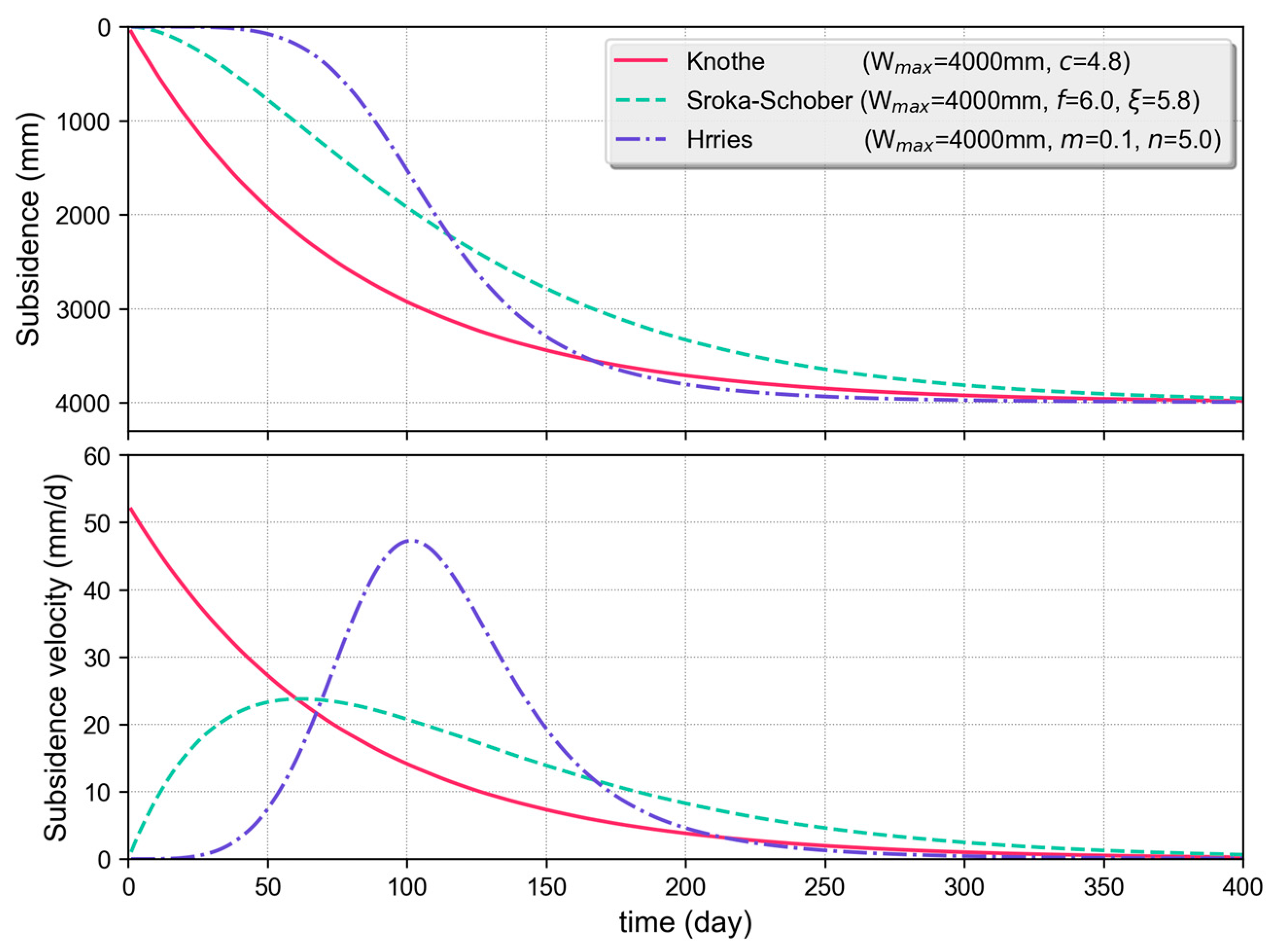
3.1. Typical Dynamic Prediction Models for Ground Subsidence

Based on the assumption that the underground coal-mining-induced ground subsidence velocity at a given time is proportional to the difference between the subsidence at that time and the maximum subsidence of the point, Knothe proposed a model (the Knothe model) to predict the dynamic ground subsidence induced by underground coal mining, which is given by [11]:

$$W(t)=W_{\max }\left(1-e^{-ct}\right)$$

(3)

where W(t) is the subsidence of a ground point at time t; W_max is the maximum subsidence at the point; c is the model coefficient, which is related to geological and mining conditions. Considering the convergence and compaction of porous rock strata, Sroka proposed a prediction model with two parameters (the Sroka–Schober model), which is given by [13]:

$$W(t)=W_{\max }\left(1+\frac{\xi }{f-\xi }{e}^{-ft}-\frac{f}{f-\xi }{e}^{-\xi t}\right)$$

(4)

where f is the relative convergence rate of the rock strata; ξ is the time coefficient of the overlying rock strata. In addition, to calculate the overlying rock subsidence, the model can also be used to predict the ground subsidence by selecting rational model parameter values. Both model parameters are in units of a⁻¹. Note that, in reality, it is impossible to measure these two model parameters directly. Based on the model describing population growth (i.e., the Gompertz model), Liu developed a ground subsidence prediction model (i.e., the Hrries model), which can be written as [24]:

$$W(t)=W_{\max }\left(1-\frac{1}{1+W_{\max }m{t}^n}\right)$$

(5)

where m and n are the model parameters with positive values.

As studied in [25,26,27], the variation pattern of subsidence induced by underground coal mining at a given ground point is very similar to a reverse “S” curve. This typical variation pattern of subsidence cannot be described by the Knothe model, as evidenced in Figure 3, which shows an example of a subsidence time series calculated using three typical models when the maximum ground subsidence is 4000 mm. The studies in [28,29] reveal that, before the ground subsidence velocity reaches its maximum, the acceleration of subsidence (second-order derivative of the subsidence time series or first-order derivative of the subsidence velocity time series) increases with respect to time; then, the acceleration of subsidence reaches its maximum at the time when the subsidence velocity equals 1/2 of the maximum subsidence velocity. Finally, the subsidence acceleration decreases to zero at the time corresponding to the maximum subsidence velocity. This is not true for the Sroka–Schober-model-described subsidence velocity time series, which has maximum subsidence acceleration when subsidence commences, as shown in the lower part of Figure 3. The Hrries model performs better in terms of the description of the empirical pattern of subsidence velocity than other two models. The reliability of the Hrries-model-based predicting result is still questioned in realistic applications, because the association between the model parameters and the geological and mining parameters is not clear [15].

3.2. Hook Function

The Hook function is a hyperbolic function similar to the inverse proportional function, which is given by [30]:

$$f_H(x)=Ax+\frac{B}{x}\hspace{1em}\mathrm{and}\hspace{1em}x\in (-\infty ,+\infty )\cap x\ne 0$$

(6)

where A and B are the function coefficients, and the coefficients satisfy:

$$A\cdot B>0$$

(7)

Clearly, the Hook function is an odd function, as shown in Figure 4, which shows an example of the Hook function in the cases of two different coefficient conditions. It can be observed from the figure that the varying pattern of the function is very different before and after the maximum (or minimum) of the function. For example, in the first case of A = 1.0 and B = 0.1, the function value decreases from +∞ to the minimum sharply with an increase in x, and then increases to +∞ slowly when the independent variable x is greater than 0.

Many field measurements show that the underground coal-mining-induced ground subsidence velocity increases sharply with the increase in time; after the velocity reaches its maximum, the velocity gradually decreases to zero [28]. In addition, the increasing pattern of the velocity is much different from the decreasing pattern of the velocity, due to the mechanism difference between underground rock collapse and compaction; specifically, the increasing rate of subsidence velocity is greater than the decreasing rate in general [29].

Obviously, the Hook function features two different varying patterns before and after the function reaches its maximum (or minimum); this can be utilized to describe the two different variation patterns of subsidence velocity, i.e., the increasing pattern and the decreasing pattern. Further, the slopes of the function are also different before and after the Hook function reaches its maximum, which is in accordance with the realistic variation pattern of subsidence acceleration. In summary, both the variation patterns of subsidence velocity and subsidence acceleration can be described by the Hook function. Thereby, the development of a subsidence velocity model based on the Hook function should be reasonable.

3.3. Proposed Dynamic Prediction Model

Before underground coal mining, the pressures or loads of the rocks are carried by the coal seam. When the coal seam is mined out, the pressures are transferred to the solid coal sides. As the mine develops with an increasing mined-out area (or goaf), the goaf progressively becomes too wide to be self-supporting. As a result, the rocks above the coal seam sag and separate along bedding planes and then fall into the goaf. After the influence of rock collapse reaches the ground surface, the ground subsidence induced by underground coal mining commences. Traditionally, for a given ground point, the whole process of underground coal-mining-induced ground subsidence can be divided into three stages: the initial stage, the active stage and the stable stage [31]. As indicated in many previous studies, once the ground point begins to be affected by the underground coal mining, the subsidence velocity increases sharply to reach its maximum, which can also be termed as the velocity increasing period (VIP). Then, the velocity decreases gradually to zero, which may take more than several years in general (or velocity decreasing period, VDP) [28]. Basically, the variation pattern of subsidence velocity can be very different for the two periods at a given ground point.

Based on the subsidence velocity variation pattern observed in many field measurements, the Hook function is utilized to describe the subsidence velocity at a ground point, which is given by:

$$v(t)=C{e}^{-f_H(t)}=C{e}^{-(At+\frac{B}{t})},\hspace{1em}\mathrm{and}\hspace{1em}t\in \left[1,+\infty \right]$$

(8)

where v(t) is the subsidence velocity of the ground point in units of mm/d; A, B and C are the coefficients of the subsidence velocity function, and the coefficients satisfy:

$$A>0;B>0;C>0$$

(9)

where t is the time in units of day, and t = 1 indicates the day when the ground point began to subside with a subsidence velocity of 1.67 mm/d. Because subsidence velocity is the derivative of the subsidence function, the subsidence function with an independent variable of t (or subsidence dynamic prediction model) can be derived from (8) by:

$$W(t)={\displaystyle {\int }_1^{t}v(t)dt}$$

(10)

where W(t) is the subsidence at a ground point in units of mm.

Figure 5 shows an example of the proposed subsidence velocity model and corresponding subsidence model in the case of three different model coefficient conditions. It can be seen from the figure that the subsidence velocity increases with the increase in time; after the velocity reaches its maximum, the velocity decreases. The differences in the subsidence velocity rates in VIP and VDP can be well described by the proposed model. In addition, the maximum subsidence velocity and varying rate of velocity in VIP and VDP can also be changed by adjusting the model coefficients with different values, which indicates the possibility of describing the realistic subsidence velocity that has occurred under different geological and mining circumstances. Further, all three subsidence curves calculated by the model present the typical reverse “S” pattern, as shown in the lower part of Figure 5, illustrating the exactness of the model in the description of the ground subsidence pattern.

3.4. Relationship between the Model Coefficients and Geological and Mining Conditions

By making the first derivative (8), one can obtain:

$$v^{\prime }(t)=\frac{dv(t)}{dt}=-C\left(A-\frac{B}{t^2}\right)e^{-(At+\frac{B}{t})}$$

(11)

Making the above equation equal to 0, the time corresponding to the maximum of the velocity function can be solved as:

$$t=t_{\max }=\sqrt{\frac{B}{A}}$$

(12)

and

$$B=A{t}_{\max }^2$$

(13)

It can be easily derived from (11) and (12) that the derivative of the velocity function is greater than 0 when t is smaller than t_max, indicating that the subsidence velocity increases with respect to t in this case; when t is larger than t_max, the derivative is less than 0, indicating that the velocity decreases with an increase in t. Further, the subsidence velocity at the ground point reaches its maximum at t_max. By substituting (12) into (8), the t_max-corresponding subsidence velocity (or the maximum subsidence velocity) can be obtained by:

$$v_{\max }=C{e}^{-2\sqrt{AB}}$$

(14)

Substituting (13) into (14), the maximum subsidence velocity can be rewritten as:

$$v_{\max }=C{e}^{-2A{t}_{\max }}$$

(15)

and

$$C=v_{\max }\cdot e^{2A{t}_{\max }}$$

(16)

The maximum subsidence of the ground point can be derived from (10) by:

$$W_{\max }={\displaystyle {\int }_1^{+\infty }v(t)dt}$$

(17)

Substituting (8) and (13) into (17), the maximum subsidence can be rewritten as:

$$W_{\max }=C{\displaystyle {\int }_1^{+\infty }{e}^{-A(t+\frac{t_{\max }^2}{t})}dt}$$

(18)

Making a ratio of (18) to (15) yields:

$$\frac{W_{\max }}{v_{\max }}=e^{2A{t}_{\max }}{\displaystyle {\int }_1^{+\infty }{e}^{-A(t+\frac{t_{\max }^2}{t})}dt}$$

(19)

By using the method of variable substitution and with some manipulations, (19) can be re-simplified as:

$$e^{2A{t}_{\max }}\cdot K_1(2A{t}_{\max })=\frac{W_{\max }}{2t_{\max }{v}_{\max }}$$

(20)

where K₁(x) is the modified Bessel function.

It can be seen from (20) that the model coefficient A is related to t_max, v_max and W_max; if the latter three parameters are known in advance, the coefficient A can be obtained by solving the implicit function with numerical methods, as detailed in [32]. Once A is obtained, the coefficients of B and C can be calculated by substituting A, t_max and v_max into (13) and (16), respectively. Clearly, the maximum subsidence W_max, maximum subsidence velocity v_max and the velocity-corresponding time t_max are the three parameters directly affecting the value of the model coefficients. Because all three parameters depend on geological and mining conditions, e.g., the mining velocity, depth of the coal seam and geological properties of the overlying rock, the model coefficients are also related to geological and mining conditions, as illustrated in Figure 6. Note that, due to the complexity of the underground coal-mining-induced ground subsidence mechanism, it is difficult to derive explicit physical meaning for a given parameter directly. However, this research theoretically derives the mathematic formula between the model parameters and the geological and mining parameters, proving the solid association between these two types of parameters; this is also a significant improvement compared with the existing models.

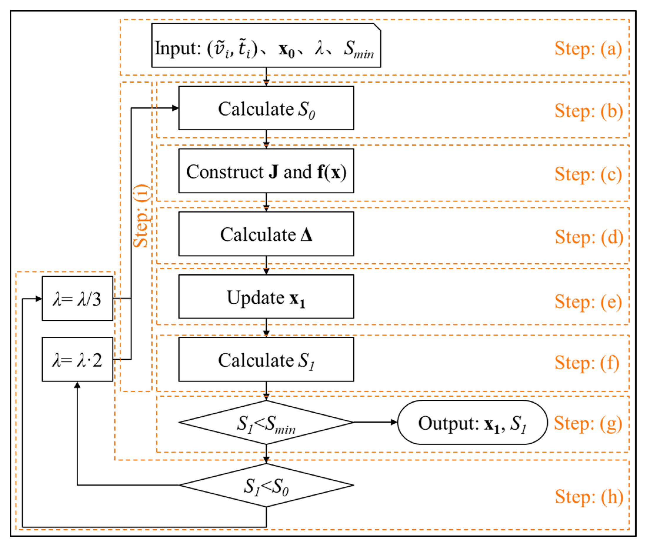
3.5. Retrieval of the Model Coefficients Using Subsidence Velocity Observations

One gives a set of subsidence velocity observations at a fixed ground point, and an equation set with three unknown model coefficients (A, B and C) can be written as:

$$\left\{\begin{array}{l}{\tilde{v}}_1=C{e}^{-(A{\tilde{t}}_1+\frac{B}{{\tilde{t}}_1})}\\ {\tilde{v}}_2=C{e}^{-(A{\tilde{t}}_2+\frac{B}{{\tilde{t}}_2})}\\ \dots \\ {\tilde{v}}_i=C{e}^{-(A{\tilde{t}}_i+\frac{B}{{\tilde{t}}_i})}\\ \dots \\ {\tilde{v}}_n=C{e}^{-(A{\tilde{t}}_n+\frac{B}{{\tilde{t}}_n})}\end{array}\right.$$

(21)

where ${\tilde{v}}_i$ is the i-th subsidence velocity observation measured on ${\tilde{t}}_i$ days after ground subsidence, and n is the number of observations. The goal of the measurement of these ground subsidence velocities is to determine the optimal model coefficients that minimize the error function:

$$\left\{\begin{array}{l}x=arg \min {\displaystyle \sum _{i=1}^n{\left[{\tilde{v}}_i-v_i(x)\right]}^2=arg \min {\displaystyle \sum _{i=1}^n{f}_i^2(x)=arg \min S}}\\ x={\left[\begin{array}{ccc}A& B& C\end{array}\right]}^T\end{array}\right.$$

(22)

Note that v_i(x) denotes the model-calculated i-th ground subsidence velocity. Obviously, this optimization problem can be treated as a non-linear least squares problem. As studied in [33], the Levenberg–Marquardt algorithm (LMA) is an effective method for solving non-linear least squares problems. Thus, the algorithm is used to determine the optimal model coefficients in the paper.

The key of LMA-based model coefficient estimation is to construct the cost function, which is given by:

$$∆={\left(J^{T}J+\lambda I\right)}^{-1}{J}^{T}f(x)$$

(23)

where λ is the damping coefficient with a nonnegative value, which can be configured as 0.1 in the case of a better initial value of A, B and C; I is the identity matrix. J is the Jacobian matrix f(x) and is given by:

$$J={\left[\begin{array}{cccccc}{J}_{A1}& J_{A2}& \cdots & J_{Ai}& \cdots & J_{An}\\ J_{B1}& J_{B2}& \cdots & J_{Bi}& \cdots & J_{Bn}\\ J_{C1}& J_{C2}& \cdots & J_{Ci}& \cdots & J_{Cn}\end{array}\right]}^T$$

(24)

and

$$J_{Ai}=\frac{\mathtt{\partial }{v}_i}{\mathtt{\partial }A}; J_{Bi}=\frac{\mathtt{\partial }{v}_i}{\mathtt{\partial }B}; J_{Ci}=\frac{\mathtt{\partial }{v}_i}{\mathtt{\partial }C}$$

(25)

The matrix f(x) is given by:

$$f(x)={\left[\begin{array}{cccccc}{f}_1(x)& f_2(x)& \cdots & f_i(x)& \cdots & f_n(x)\end{array}\right]}^T$$

(26)

In addition, the initial value of the model coefficient is important for improving the efficiency and optimization performance of the LMA. In reality, the maximum subsidence of a given ground point (i.e., W_max) can be estimated by using the static prediction model (e.g., the probability integration model) based on the actual mining and geological parameters. The maximum subsidence velocity (v_max) can be related to the mining parameters by using the empirical formula [34]:

$$v_{\max }\approx \frac{K{W}_{\max }V}{H_0}$$

(27)

where K is the subsidence-velocity-related coefficient, which is in the range of 0.5 to 3.0; V is the average mining velocity of the working face; and H₀ is the average coal seam depth. The time corresponding to the maximum subsidence velocity (t_max) depends on the advancing and lagging influence distance of the coal seam, which can be calculated approximately by:

$$t_{\max }\approx \frac{d_A+d_L}{V}$$

(28)

where d_A and d_L are the advancing and lagging influence distance of the coal seam, respectively. Once the approximations of the model coefficients are determined by the mining and geological conditions of the working face, the initial values of the model coefficients can be calculated through (13), (16) and (20), respectively.

Based on the optimization formula of (23) and the initial value of the model coefficients, the LMA-based optimal model coefficient inversion algorithm can be developed. A flowchart of the algorithm is shown in Figure 7. The algorithm process is described as follows:

(a)

Input the observation series of ground subsidence velocity, initial values of the model coefficients, damping coefficient and limit error S_min.

(b)

Calculate the residual sum of the squares between the observed and predicted results S₀ using the observation series and initial model coefficients based on (22).

(c)

Construct the Jacobian matrix J and residual matrix f(x) using (24) and (26), respectively.

(d)

Calculate the cost function matrix ∆ using (23).

(e)

Update the optimal prediction model coefficients by:

$$x_1=x_0-\mathbf{∆}$$

(29)

(f)

Calculate the residual sum of the squares between the observed and predicted results S₁ with the updated model coefficients x₁.

(g)

If S₁ is less than the limit error S_min, output the updated model coefficients and the residual sum of the squares.

(h)

If S₁ > S_min and S₁ < S₀, increase λ twofold; otherwise, decrease λ threefold.

(i)

Assign the updated prediction model coefficients and the damping coefficient to the corresponding initial coefficient and return to step (b).

4. Results

The GNSS subsidence velocity observations collected in the active stage of ground subsidence were used to validate the proposed subsidence velocity model, i.e., Equation (8). One-third of the velocity observations were taken as the modeling datasheet to calculate the optimal model coefficients with the method detailed in Section 3.5, and the other observations were taken as the validating datasheet to evaluate the precision of the model. A comparison between the subsidence velocity time series of the modeling datasheet and that of the model-fitted datasheet for four GNSS stations is shown in the upper part of Figure 8; a scatterplot of the modeling datasheet versus the model-fitted one is shown in the upper part of Figure 9. A comparison between the subsidence velocity time series of the validating datasheet and that of the model-fitted one for these stations is shown in the lower part of Figure 8; a scatterplot of the validating datasheet versus the model-fitted one is shown in the lower part of Figure 9. The RMSs of the model-fitted subsidence velocity error for the modeling datasheet and validating datasheet are shown in

Table 1. Mean, STD and RMS of model-fitted subsidence velocity error for modeling datasheet.

Station	Mean (mm/d)	STD (mm/d)	RMSE (mm/d)	vmax (mm/d)
CRS01	0.03	0.98	0.98	12.57
CRS02	0.13	2.11	2.12	29.64
CRS03	0.79	5.12	5.23	78.30
CRS04	0.31	5.37	5.38	82.70
All	0.34	4.23	4.24	82.70

and

Table 2. Mean, STD and RMS of model-fitted subsidence velocity error for validating datasheet.

Station	Mean (mm/d)	STD (mm/d)	RMSE (mm/d)	vmax (mm/d)
CRS01	0.02	0.95	0.95	12.51
CRS02	0.16	2.10	2.11	30.17
CRS03	0.76	5.17	5.23	78.30
CRS04	0.31	5.22	5.23	83.04
All	0.34	4.17	4.18	83.04

, respectively. By fitting the subsidence velocity observations in VIP with a linear function, the subsidence velocity increasing rate (SVIR) could be approximately obtained. Similarly, the subsidence velocity decreasing rate (SVDR) could also be obtained by fitting the subsidence velocity observations in VDP with a linear function. The SVIR and SVDR for these four GNSS stations are shown in

Table 3. SVIR and SVDR for four GNSS stations.

Station	SVIR (mm/d2)	SVDR (mm/d2)	Mining Velocity (m/d)
CRS01	2.72	−0.80	3.5
CRS02	2.79	−0.83	3.2
CRS03	5.76	−1.11	4.3
CRS04	2.73	−0.80	1.4

.

By substituting the modeling-datasheet-calculated model coefficients into (10), the ground subsidence at each time point could be obtained. A comparison of the time series between the GNSS-observed ground subsidence and the model-predicted one for the four stations during the experimental campaign is shown in Figure 10. A scatterplot of the GNSS-observed ground subsidence and the model-predicted subsidence for these four stations is shown in Figure 11. Taking the GNSS-observed ground subsidence as the in situ data, the mean, STD and RMS of the model-predicted ground subsidence error could be calculated and are shown in

Table 4. Mean, STD and RMS of model-predicted subsidence error for four GNSS stations.

Station	Mean (mm)	STD (mm)	RMSE (mm)	Wmax (mm)	MRE (%)
CRS01	−36.0	21.2	41.8	808.0	8.3
CRS02	−60.5	47.9	77.2	1678.1	7.6
CRS03	−11.3	54.4	55.6	3911.0	3.7
CRS04	−9.0	39.4	40.4	5820.7	2.5
All	−29.8	47.5	56.1	5820.7	2.5

.

5. Discussion

5.1. Ground Subsidence Velocity

It can be seen from Figure 8 and Table 3 that the ground subsidence velocity increased sharply with an SVIR greater than 2 mm/d², once the ground began to be affected by the underground coal mining. The velocity decreased to zero with a comparatively gradual pattern after the velocity reached its maximum; the SVDR was greater than −1.5 mm/d² for all four stations. Basically, the SVIR was proportional to the maximum subsidence velocity v_max; with the increase in the maximum velocity, the SVIR increases. For example, the maximum subsidence velocity was 12.51 mm/d, 30.17 mm/d and 78.30 mm/d for the CRS01, CRS02 and CRS03 stations, respectively, as shown in Table 2, while the corresponding increasing rates were 2.72 mm/d², 2.79 mm/d² and 5.76 mm/d², as shown in Table 3. Similarly, the absolute value of the SVDR was also proportional to the maximum subsidence velocity, and the magnitude of SVDR was much smaller than that of the SVIR for each GNSS station; e.g., the SVIR and absolute value of the SVDR were 5.76 mm/d² and 1.11 mm/d^2, respectively, for the CRS03 station. This also indicates that the ground surface would take more time to resume a stable status, i.e., the subsidence velocity decreases to 0 mm/d.

It is important to note that the SVIR and absolute value of SVDR at the CRS04 station were significantly less than that at the CRS03 station, although the difference in the maximum subsidence velocities was marginal for these two stations. The main reason should be attributed to the difference in mining velocities. As studied in [35], the faster loss of subsurface volume is the main factor inducing the increased ground subsidence; therefore, the intensity of the ground deformation is proportional to the underground coal mining velocity in general. With the increase in the mining velocity, the ground deformation becomes more drastic; therefore, the increment in the subsidence velocity (SVIR and SVDR) increases significantly. The in situ mining velocity of the working face was about 4.3 m/d around the CRS03 station, as shown in Table 3, while the mining velocity was about 1.4 m/d around the CRS04 station, which is much smaller than that at the CRS03 station. Because of the lower mining velocity, the subsidence of the ground surface around the CRS04 station was comparatively gradual; therefore, the SVIR and absolute value of SVDR at CRS04 were less than those at CRS03. This observation is useful because we can intentionally control the mining velocity to decrease the intensity of the ground subsidence and, therefore, damage to the ground surface buildings. In addition, it can be observed from (8) that the ground subsidence velocity is proportional to the parameter A and is inversely proportional to the exponential of parameters B and C. Thus, one can easily infer that the influence of parameter A on the subsidence-predicting results is less than that of B and C.

In general, there exists good accordance between the GNSS-observed subsidence velocity and the model-fitted one, as shown in Figure 8 and Figure 9. The minimum and maximum correlation coefficients between the observed velocity and the model-fitted one are 0.965 and 0.984 for the modeling results and are 0.969 and 0.983 for the validating results, which indicates a very strong correlation between the GNSS-observed and the model-fitted subsidence velocity. For the entire modeling datasheet, the mean, STD and RMS of the model-fitted velocity error are 0.34 mm/d, 4.23 mm/d and 4.24 mm/d, respectively; the model has similar estimating precision for the validating datasheet, as shown in Table 1 and Table 2. By making a ratio of the absolute error of the model-calculated subsidence velocity to the observed maximum subsidence velocity, the relative error of the model-calculated subsidence velocity estimation can be obtained. The maximum relative errors of the model-calculated subsidence velocity are 21.9% and 23.1% for the modeling datasheet and the validating datasheet, respectively. To some extent, the error between the model-calculated subsidence velocity and the GNSS-observed one is slightly larger. Despite this, it can be seen from Table 1 and Table 2 that the error is mainly composed of the random error (or STD); for example, the STD and RMS of the model-calculated subsidence velocity estimating error are 4.17 mm/d and 4.18 mm/d for the validating datasheet. Because subsidence is the integral of subsidence velocity with respect to time and the integral operation can significantly decrease the influence of the random error, as analyzed in [36], the proposed model would still have strong performance for subsidence prediction, as proved in the next section.

5.2. Dynamic Ground Subsidence

Underground coal-mining-induced subsidence at the surface develops progressively. For a given observation point on the ground surface, a slight downward movement on the point becomes detectable when the working face is behind the point with a distance of about 100 to 300 m. As the coal mining working face passes beneath the point, the subsidence increases rapidly. When the working face is ahead of the point with a distance of about 50 to 150 m, the subsidence velocity of the point reaches its maximum and then decreases obviously with the termination of the re-adjustment of the underlying strata. As a result, the subsidence on the point increases continuously and gradually approaches the maximum magnitude; the subsidence process may last for several years or decades. Basically, the subsidence curve at a ground point with respect to time is very close to an inverse S-shaped curve, as revealed in many previous studies [25,26]. It can be seen from Figure 10 that the GNSS-observed and the model-predicted subsidence curves have good accordance with these previous studies for all four stations; i.e., the time series of the subsidence presents as an inverse S-shaped curve in general.

Further, it can also be observed from Figure 10 that the maximum subsidence can be significantly different for different stations. This was mainly caused by a difference in GNSS station locations relative to the working face. In reality, underground coal-mining-induced ground subsidence is a complex temporal and spatial process. In the spatial dimension, underground coal mining can induce a bowl-shaped subsidence basin on the ground surface, and the area of the basin is much greater than the mined area. For a given ground point on the subsidence basin, the magnitude of subsidence of the point is inversely proportional to the horizontal distance from the point to the center of the goaf. The distance is about 645 m, 480 m, 203 m and 89 m for CRS01, CRS02, CRS03 and CRS04, respectively. Apparently, the maximum subsidence on these stations can increase in sequence. This can also be seen clearly from Table 4; e.g., the GNSS-observed maximum subsidence on these four stations is 808.0 mm, 1678.1 mm, 3911.0 mm and 5820.7 mm, respectively.

The model-predicted subsidence time series is very close to that observed by the GNSS station, indicating a good accordance between the two results. The linear correlation coefficient between the model-predicted and GNSS-observed subsidence is greater than 0.99 for all four GNSS stations, as shown in Figure 11, which also proves the good performance of the developed model. The RMS of the model-predicted subsidence error is 41.8 mm, 77.2 mm, 55.6 mm and 40.4 mm for CRS01, CRS02, CRS03 and CRS04, respectively; the RMSE is 56.1 mm for all GNSS observations, as shown in Table 4. By making a ratio of the absolute error of the model-predicted subsidence to the GNSS-observed maximum subsidence, the relative error of the model-predicted ground subsidence can be obtained. The maximum relative errors (MREs) are 8.3%, 7.6%, 3.7% and 2.5% for CRS01, CRS02, CRS03 and CRS04, respectively. It can also be observed from Table 4 that the MRE is inversely proportional to the maximum subsidence; i.e., with the increase in the maximum subsidence, the MRE decreases significantly. This is because the difference in the model-predicted absolute error (i.e., numerator of the MRE) is slight in the cases of different subsidence magnitudes, while with the increase in the maximum subsidence (i.e., denominator of the MRE), the MRE decreases. Basically, for ground subsidence dynamic predictions, a relative error less than 15% is enough for many realistic engineering applications, such as the evaluation of building damage degree or the design of remediation plans for the subsidence basin [37]. Clearly, the accuracy of the proposed model-predicted dynamic subsidence can satisfy the criterion, especially when the maximum subsidence is greater than 3000 mm.

5.3. Gap between the Proposed Method and the Existing Methods

At present, the prediction of ground subsidence induced by underground coal mining is a popular research direction. This prediction can be divided into two types: static subsidence prediction and dynamic subsidence prediction. The former mainly includes influence function methods, full-scale subsidence fitting methods and simulation methods [38], and the prediction has been well studied in the last eighty years. However, research related to the dynamic subsidence method has been limited until now due to the lack of field measurements with high temporal resolution. Basically, the existing dynamic subsidence method can be divided into three types: a time function method, numerical method, and machine learning method, as shown in

Table 5. Comparison of advantages and disadvantages between the proposed method and the existing methods.

Type	Time Function Method	Numerical Method	Machine Learning Method
Typical method	Knothe model Kowalski model Sroka–Schober model Hrries model	FLAC3D simulation 3DEC simulation	Neural network model Support vector machine model Random forest model
Advantages	Fewer modeling data Explicit function expression Moderate prediction accuracy	Describes the mechanical mechanism of ground subsidence well	High prediction accuracy
Disadvantages	Weak association between model parameters and geological and mining parameters Incapable of describing the mechanical mechanism of ground subsidence	Inferior prediction accuracy	Large volume of modeling data Inexplicit function expression Incapable of describing the mechanical mechanism of ground subsidence

. The typical time function methods include the Knothe model, Kowalski model, Sroka–Schober model and Hrries model. The method can make use of fewer field measurements to develop an explicit subsidence prediction function with moderate accuracy. However, as mentioned in the previous section, the association between the function parameters and geological and mining parameters is not clear for many existing prediction models; in addition, the time function methods are incapable of describing the mechanical mechanism of ground subsidence. The numerical methods include the FLAC3D and 3DEC simulating method; the mechanical mechanism of ground subsidence can be well described by the method, although the subsidence prediction accuracy is usually inferior in reality due to the difficulty of measuring the in situ mechanical parameters of rocks and soils [39,40,41]. In recent years, machine learning methods, such as the neural network model, support vector machine model and random forest model, have also been used to develop the dynamic subsidence prediction model [42,43,44,45]. The method-based subsidence prediction accuracy is rather high in general. However, machine learning methods need a large number of field measurements to adjust the models, which is the key factor restricting research into the method. In addition, similar to the time function methods, the machine learning methods are also incapable of describing the mechanical mechanism of ground subsidence. According to the classification shown in Table 5, the proposed method is a time function method and possesses the advantages and disadvantages associated with time function methods in general. In addition, different from the existing time function methods, the coefficients of the developed model can be easily associated with the geological and mining parameters, which is a significant improvement compared with the existing time function models. Also, due to the development of the model based on the subsidence velocity, the dynamic variations in both the ground subsidence and subsidence velocity can be well described using the proposed method.

It is important to note that all existing subsidence prediction methods were developed based on the premise that the ground subsidence induced by underground coal mining varies continuously. These models predict that ground subsidence could produce an obvious deviation in the case of the discontinuous subsidence of the ground surface (e.g., ground cracks due to the stretching deformation of the ground surface). This is also true for the proposed method; that is, the proposed method might be invalid when the surface’s discontinuous deformation is serious.

6. Conclusions

In this paper, a new model was developed to predict the dynamic ground subsidence induced by underground coal mining. Different from the previous modeling methods, which develop a mathematic formula describing the relationship between subsidence and time directly, the proposed method develops a formula describing the relationship between the derivative of subsidence (or subsidence velocity) and time using the Hook function; the integral of the formula is treated as the ground subsidence dynamic prediction model. Thereby, both ground subsidence and subsidence velocity characteristics can be well described by the developed model. In addition, the model coefficients are concise and related to geological and mining conditions, which makes the model more applicable in reality. Based on the Levenberg–Marquardt algorithm, an inversion method was also proposed to calculate the optimal model coefficients with the subsidence velocity observations. The developed model was validated and analyzed comprehensively with GNSS observations collected in an experimental campaign conducted in a typical longwall coal mining working face of the Jining mining area, China, over two years. The main conclusions of this paper are summarized as follows:

(a)

The acceleration of ground subsidence (or a derivative of subsidence velocity) is related to the maximum subsidence velocity at the ground point and the mining velocity; the acceleration is proportional to the two velocities. Thus, decreasing the mining velocity artificially is an effective way to control the intensity of ground perturbations induced by underground coal mining.

(b)

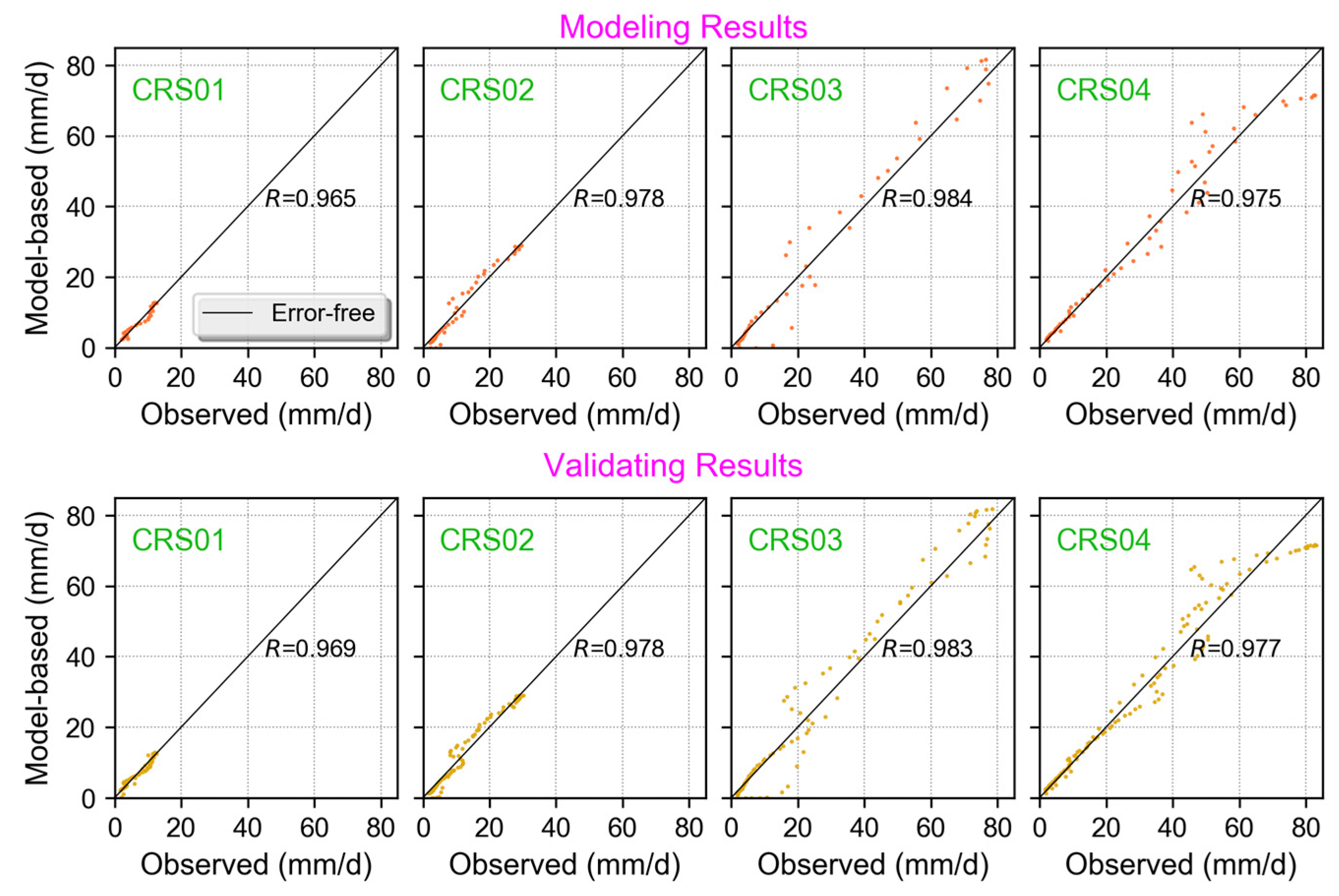
The developed model can be used to predict the subsidence velocity well. When the maximum subsidence velocity is less than 80 mm/d, the RMS of the model-predicted subsidence velocity error is 4.18 mm/d; the maximum relative error for the model-predicted subsidence velocity is 23.1%.

(c)

In addition to subsidence velocity, the model can also predict ground subsidence accurately. When the maximum ground subsidence is less than 6000 mm, the RMS of the model-predicted subsidence error is 56.1 mm; the maximum relative error for the model-predicted subsidence is 2.5%.

Future research will focus on a combination of the proposed model and the existing models (e.g., the probability integration model) to predict dynamic subsidence over the whole subsidence basin. In addition, dynamic subsidence prediction with high accuracy is of great importance for the dynamic reclamation of subsidence land caused by underground coal mining; a comprehensive evaluation of the proposed method and the existing methods using field measurements collected in different areas is another future research focus.

References

1. Zhang, C.; Zhong, L.; Fu, X.; Zhao, Z. Managing Scarce Water Resources in China’s Coal Power Industry. Environ. Manag. 2016, 57, 1188–1203. [Google Scholar] [CrossRef] [PubMed]
2. Bell, F.G.; Stacey, T.R.; Genske, D.D. Mining subsidence and its effect on the environment: Some differing examples. Environ. Geol. 2000, 40, 135–152. [Google Scholar] [CrossRef]
3. Kay, D.J. Managing mine subsidence along railways and highway pavements in the southern coalfield. J. News Aust. Geomech. Soc. 2012, 47, 33–52. [Google Scholar]
4. Karanam, V.; Motagh, M.; Garg, S.; Jain, K. Multi-sensor remote sensing analysis of coal fire induced land subsidence in Jharia Coalfields, Jharkhand, India. Int. J. Appl. Earth Obs. Geoinf. 2021, 102, 102439. [Google Scholar] [CrossRef]
5. Li, L.; Li, W.; Wang, Q. Prediction and zoning of the impact of underground coal mining on groundwater resources. Process Saf. Environ. Prot. 2022, 168, 454–462. [Google Scholar] [CrossRef]
6. Fan, G.; Zhang, D. Mechanisms of Aquifer Protection in Underground Coal Mining. Mine Water Environ. 2015, 34, 95–104. [Google Scholar] [CrossRef]
7. Badrul Alam, A.K.M.; Fujii, Y.; Eidee, S.; Boeut, S.; Rahim, A.B. Prediction of mining-induced subsidence at Barapukuria longwall coal mine, Bangladesh. Sci. Rep. 2022, 12, 14800. [Google Scholar] [CrossRef]
8. Zhang, S.; Zhang, J. Ground Subsidence Monitoring in a Mining Area Based on Mountainous Time Function and EnKF Methods Using GPS Data. Remote Sens. 2022, 14, 6359. [Google Scholar] [CrossRef]
9. Cheng, H.; Zhang, L.; Guo, L.; Wang, X.; Peng, S. A New Dynamic Prediction Model for Underground Mining Subsidence Based on Inverse Function of Unstable Creep. Adv. Civ. Eng. 2021, 2021, 9922136. [Google Scholar] [CrossRef]
10. He, L.; Wu, D.; Ma, L. Numerical simulation and verification of goaf morphology evolution and surface subsidence in a mine. Eng. Fail. Anal. 2023, 144, 106918. [Google Scholar] [CrossRef]
11. Knothe, S. Effect of time on formation of basin subsidence. Arch. Min. Steel Ind. 1953, 1, 1–7. [Google Scholar]
12. Peng, X.; Cui, X.; Zang, Y.; Wang, Y.; Yuan, D. Time function and prediction of progressive surface movement sand deformations. J. Univ. Sci. Technol. Beijing 2004, 26, 341–344. [Google Scholar]
13. Kwinta, A.; Hejmanowski, R.; Sroka, A. Time function analysis used for the prediction of rock mass subsidence. In Proceedings of the International Symposium on Mining Science and Technology, Xuzhou, China, 16 October 1996; pp. 419–424. [Google Scholar]
14. Liu, Y. Dynamic surface subsidence curve model based on Weibull time function. Rock Soil Mech. 2013, 34, 2409–2413. [Google Scholar]
15. Han, J.; Hu, C.; Zou, J. Time Function Model of Surface Subsidence Based on Inversion Analysis in Deep Soil Strata. Math. Probl. Eng. 2020, 2020, 4279401. [Google Scholar] [CrossRef]
16. Liu, C.; Gao, J.; Yu, X.; Zhang, J.; Zhang, A. Mine surface deformation monitoring using modified GPS RTK with surveying rod: Initial results. Surv. Rev. 2015, 47, 79–86. [Google Scholar] [CrossRef]
17. Mcclusky, S.; Balassanian, S.; Barka, A.; Demir, C.; Ergintav, S.; Georgiev, I.; Gurkan, O.; Hamburger, M.; Hurst, K.; Kahle, H.; et al. Global Positioning System constraints on plate kinematics and dynamics in the eastern Mediterranean and Caucasus. J. Geophys. Res. 2000, 105, 5695–5719. [Google Scholar] [CrossRef]
18. Wang, J.; Peng, X.; Xu, C. Coal mining GPS subsidence monitoring technology and its application. Min. Sci. Technol. (China) 2011, 21, 463–467. [Google Scholar] [CrossRef]
19. Gao, J.; Liu, C.; Wang, J.; Li, Z.; Meng, X. A new method for mining deformation monitoring with GPS-RTK. Trans. Nonferrous Met. Soc. China 2011, 21, s659–s664. [Google Scholar] [CrossRef]
20. Li, X.; Wang, B.; Li, X.; Huang, J.; Lyu, H.; Han, X. Principle and performance of multi-frequency and multi-GNSS PPP-RTK. Satell. Navig. 2022, 3, 1–11. [Google Scholar] [CrossRef]
21. Herring, T.A.; Melbourne, T.I.; Murray, M.H.; Floyd, M.A.; Szeliga, W.M.; King, R.W.; Phillips, D.A.; Puskas, C.M.; Santillan, M.; Wang, L. Plate Boundary Observatory and related networks: GPS data analysis methods and geodetic products. Rev. Geophys. 2016, 54, 759–808. [Google Scholar] [CrossRef]
22. Gao, J.; Hong, H. Advanced GNSS technology of mining deformation monitoring. Procedia Earth Planet. Sci. 2009, 1, 1081–1088. [Google Scholar]
23. Yang, D.; Zou, J. Precise levelling in crossing river over 5 km using total station and GNSS. Sci. Rep. 2021, 11, 7492. [Google Scholar] [CrossRef] [PubMed]
24. Liu, X.; Wang, J.; Guo, J.; Yuan, H.; Li, P. Time function of surface subsidence based on Harris model in mined-out area. Int. J. Min. Sci. Technol. 2013, 23, 245–248. [Google Scholar] [CrossRef]
25. Liu, X.; Xu, L.; Zhang, K. Strata Movement Characteristics in Underground Coal Gasification (UCG) under Thermal Coupling and Surface Subsidence Prediction Methods. Appl. Sci. 2023, 13, 5192. [Google Scholar] [CrossRef]
26. Mehrabi, A.; Derakhshani, R.; Nilfouroushan, F.; Rahnamarad, J.; Azarafza, M. Spatiotemporal subsidence over Pabdana coal mine Kerman Province, central Iran using time-series of Sentinel-1 remote sensing imagery. Episodes 2023, 46, 19–33. [Google Scholar] [CrossRef]
27. Przylucka, M.; Kowalski, Z.; Perski, Z. Twenty years of coal mining-induced subsidence in the Upper Silesia in Poland identified using InSAR. Int. J. Coal Sci. Technol. 2022, 9, 86. [Google Scholar] [CrossRef]
28. Yan, W.; Chen, J.; Tan, Y.; He, R.; Yan, S. Surface Dynamic Damage Prediction Model of Horizontal Coal Seam Based on the Idea of Wave Lossless Propagation. Int. J. Environ. Res. Public Health 2022, 19, 6862. [Google Scholar] [CrossRef]
29. Behera, A.; Rawat, K.S. A brief review paper on mining subsidence and its geo-environmental impact. Mater. Today Proc. 2023; in press. [Google Scholar] [CrossRef]
30. Virtanen, P.; Gommers, R.; Oliphant, T.E.; Haberland, M.; Reddy, T.; Cournapeau, D.; Burovski, E.; Peterson, P.; Weckesser, W.; Bright, J.; et al. SciPy 1.0: Fundamental Algorithms for Scientific Computing in Python. Nat. Methods 2020, 17, 261–272. [Google Scholar] [CrossRef] [PubMed]
31. Zhang, L.; Cheng, H.; Yao, Z.; Wang, X. Application of the Improved Knothe Time Function Model in the Prediction of Ground Mining Subsidence: A Case Study from Heze City, Shandong Province, China. Appl. Sci. 2020, 10, 3147. [Google Scholar] [CrossRef]
32. Meurer, A.; Smith, C.P.; Paprocki, M.; Čertík, O.; Kirpichev, S.B.; Rocklin, M.; Kumar, A.; Ivanov, S.; Moore, J.K.; Singh, S.; et al. SymPy: Symbolic computing in Python. PeerJ Comput. Sci. 2017, 3, e103. [Google Scholar] [CrossRef]
33. Livet, C.; Rouvier, T.; Sauret, C.; Pillet, H.; Dumont, G.; Pontonnier, C. A penalty method for constrained multibody kinematics optimisation using a Levenberg–Marquardt algorithm. Comput. Methods Biomech. Biomed. Eng. 2023, 26, 864–875. [Google Scholar] [CrossRef] [PubMed]
34. Guo, W.; Bai, E.; Yang, D. Surface subsidence characteristics and damage protection techniques of high-intensity mining in China. Adv. Coal Mine Ground Control. 2017, 157–203. [Google Scholar] [CrossRef]
35. Li, H.; Qi, Q.; Du, W.; Li, X. A criterion of rockburst in coal mines considering the influence of working face mining velocity. Geomech. Geophys. Geo-Energy Geo-Resour. 2022, 8, 37. [Google Scholar] [CrossRef]
36. Howitt, G.D.; Luus, R. Model reduction by minimization of integral square error performance indices. J. Frankl. Inst. 1990, 327, 343–357. [Google Scholar] [CrossRef]
37. Donnelly, L.J.; Cruz, D.; Asmar, I.; Zapata, O.; Perez, J.D. The monitoring and prediction of mining subsidence in the Amaga, Angelopolis, Venecia and Bolombolo Regions, Antioquia, Colombia. Eng. Geol. 2001, 59, 103–114. [Google Scholar] [CrossRef]
38. Cai, Y.; Jin, Y.; Wang, Z.; Chen, T.; Wang, Y.; Kong, W.; Xiao, W.; Li, X.; Lian, X.; Hu, H. A review of monitoring, calculation, and simulation methods for ground subsidence induced by coal mining. Int. J. Coal Sci. Technol. 2023, 10, 32. [Google Scholar] [CrossRef]
39. Li, H.; Zha, J.; Guo, G. A new dynamic prediction method for surface subsidence based on numerical model parameter sensitivity. J. Clean. Prod. 2019, 233, 1418–1424. [Google Scholar] [CrossRef]
40. Jing, L. A review of techniques, advances and outstanding issues in numerical modelling for rock mechanics and rock engineering. Int. J. Rock Mech. Min. Sci. 2003, 40, 283–353. [Google Scholar] [CrossRef]
41. Ma, F.; Yang, F. Research on numerical simulation of stratum subsidence. J. Liaoning Tech. Univ. (Nat. Sci.) 2001, 20, 257–261. [Google Scholar]
42. Liu, X.; Zhao, Y.; Zhou, F. Dynamic prediction of mining-induced subsidence based on a hybrid model. J. Min. Saf. Eng. 2020, 37, 163–170. [Google Scholar]
43. Wang, J.; Wang, X. Dynamic prediction of mining-induced subsidence using a neural network model. Arab. J. Geosci. 2017, 10, 170–192. [Google Scholar]
44. Wang, K.; Wang, L. Time function analysis of mining-induced subsidence based on a backpropagation neural network. J. Appl. Geophys. 2018, 157, 57–65. [Google Scholar]
45. Yang, Q.; Tang, H.; Wang, X. Dynamic prediction of mining-induced subsidence based on a random forest model. J. Min. Saf. Eng. 2018, 35, 350–356. [Google Scholar]
Figure 1. Location and GNSS station distribution of the study area.
Remotesensing 16 00377 g001
Figure 2. Comparison between the GNSS-based ground subsidence and the leveling-based one.
Remotesensing 16 00377 g002
Figure 3. Three typical models for underground coal-mining-induced subsidence (upper) and subsidence velocity (lower) prediction results.
Remotesensing 16 00377 g003
Figure 4. Example of Hook function in the cases of two different coefficient conditions.
Remotesensing 16 00377 g004
Figure 5. Examples of the proposed prediction model for ground subsidence velocity (upper) and ground subsidence (lower) in the cases of different coefficient conditions.
Remotesensing 16 00377 g005
Figure 6. Relationship between the model coefficients and geological and mining conditions.
Remotesensing 16 00377 g006
Figure 7. LMA-based flowchart for inversion of optimal model coefficients.
Remotesensing 16 00377 g007
Figure 8. Time series comparison between the observed subsidence velocity and that of the model-fitted one for the modeling datasheet (upper) and the validating datasheet (lower).
Remotesensing 16 00377 g008
Figure 9. Scatterplot of the observed subsidence velocity versus the model-fitted one for the modeling datasheet (upper) and the validating datasheet (lower).
Remotesensing 16 00377 g009
Figure 10. Time series of the GNSS-based ground subsidence observation versus the model-predicted subsidence for four stations.
Remotesensing 16 00377 g010
Figure 11. Scatterplot of the GNSS-based ground subsidence observation versus the model-predicted subsidence for four stations.
Remotesensing 16 00377 g011