1. Introduction
High frequency surface wave radar (HFSWR) can provide the capabilities of over-the-horizon detection and ocean remote sensing by transmitting vertically polarized electromagnetic waves working in the high-frequency band of 3–30 MHz. It is an integrated maritime surveillance system because of its notable features of high Doppler frequency resolution, long distance, and all-day adaptability [
1]. However, the target detection performance of the HFSWR system depends highly on the distribution of external environmental noise, the principal components of which consist of cosmic noise, man-made noise, and atmospheric noise [
2]. Especially in the high frequency (HF) band, this external environment noise has a complex behavior that varies with geographic location, time of day, season, solar activity cycle, and operating frequency [
3,
4]. Previous studies generally considered that HF external environmental noise is omnidirectional in azimuth [
5,
6]. However, the spatial distribution of the external environment’s noise intensity is directional due to severe weather on the sea surface (such as lightning and typhoons) or human factors (such as industrial or residential areas), called directional noise [
7,
8,
9,
10]. As for radar systems, detecting weak targets of interest emerging into directional noise is a new challenge.
HF external environment noise has been an important research subject. In the 1930s, many measurements and research on HF noise were started in Europe [
11,
12,
13,
14]. However, the results are controversial due to the limitations of the equipment and the lack of standardization of measurement methods. HF noise was generally modeled as Gaussian noise, color noise, or a mixture of pulse noise and discrete interference components [
15]. Most of the modeling and measurement experiments of HF external environmental noise were focused on its temporal or statistical characteristics, with little consideration of its spatial directional distribution. The standard HF environment noise model was released by the International Telecommunication Union (ITU) in 1990, providing only a fairly rough result for noise distribution [
16,
17]. Based on the ITU model, Kotaki first developed an HF external environmental noise model based on the global lightning strike activity distribution [
18]. Unfortunately, both the Kataki and ITU models failed to provide information about noise directionality distribution. However, a strong directional characteristic is supported by observations from the HFSWR receiver [
10]. Coleman first proposed an HF directional noise model based on global maps of lightning strike occurrence and ray tracing propagation methods [
7]. Pederick combined background ionosphere and ionospheric absorption models based on the Coleman model, which can simulate the directional noise more accurately [
8]. The simulated results agree well with the Jindalee Operational Radar Network (JORN) radar measurements, matching the results more closely than the standard ITU noise model. Gibson and Arnett carried out some research on the directional distribution of HF noise at a measuring site in Southern England [
19]. The results showed the greatest asymmetry in noise intensity during the spring or summer evening, and the results were also generally consistent with the expected distribution of atmospheric noise caused by thunderstorm activity at that time.
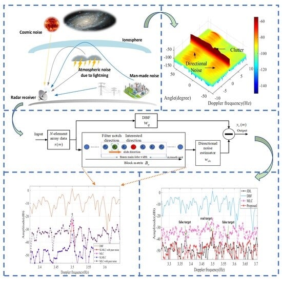
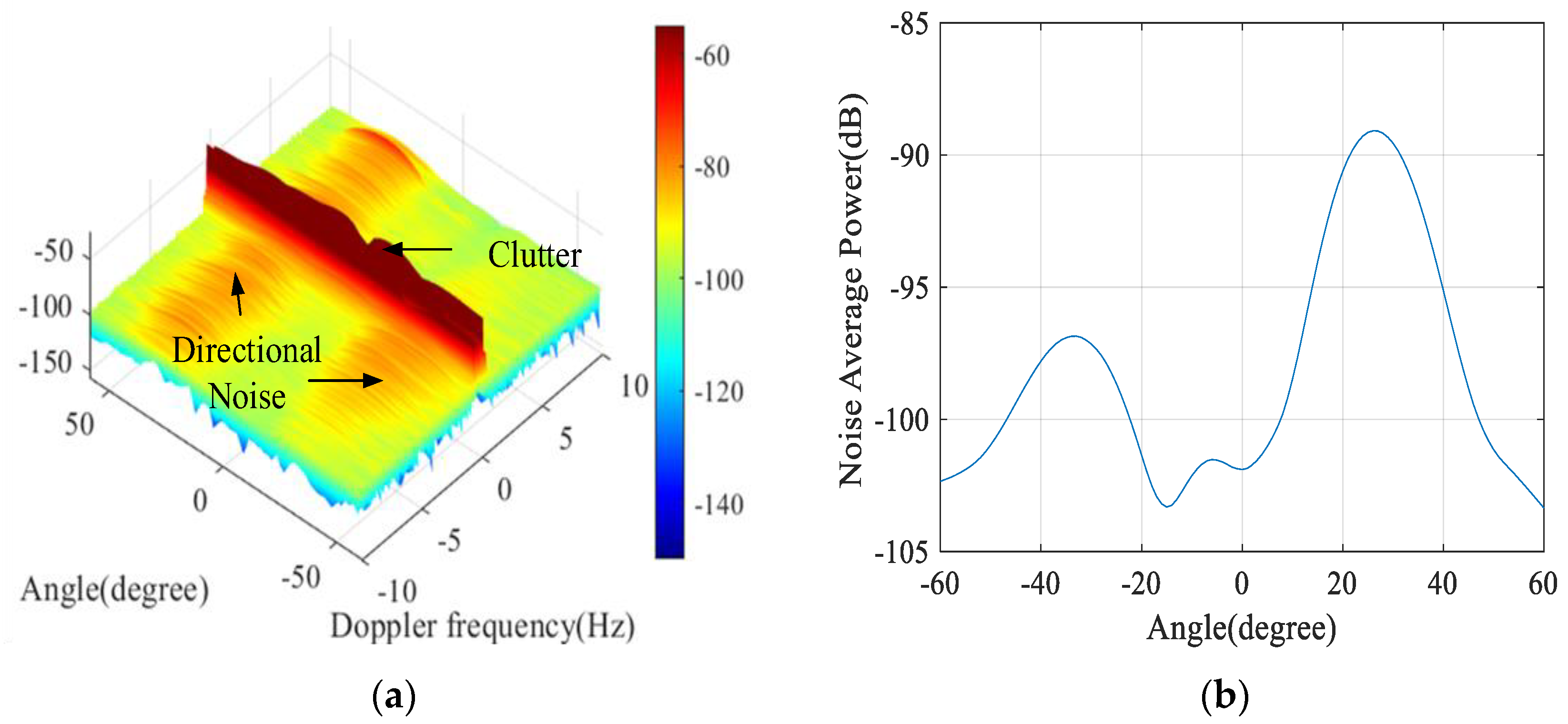
At HF, external environmental noise originates mainly from three sources, as shown in
Figure 1. The atmospheric component is driven by lightning strikes, which can be separated into two components: a local component (which propagates via ground waves or line-of-sight, for example, when local thunderstorm activity is within 100 km of the HFSWR receiver) and an ionospheric component. The ionospheric component results from the superposition of many lightning strikes across the globe. The electromagnetic radiation from lightning strikes will be reflected in the ionosphere [
20,
21]. Under certain propagation conditions, this portion of radiation can be received by the radar receiver after a second reflection via the ionosphere. Man-made noise is caused by electrical and electronic equipment, power transmission lines, combustion engine ignition, power line telecommunications, and switching power. Due to the high equipment density in cities and their proximity, noise levels are high [
22]. This noise reaches the receiver by direct coupling, line-of-sight, or groundwave propagation, depending on distance and frequency. In addition, the effect of man-made noise propagated via ground waves depends on the location of the noise source relative to the radar; it has location uniqueness [
23]. Another source is cosmic noise, which originates from extraterrestrial space and needs to propagate through the ionosphere. This noise is only present at higher frequencies or high elevation angles, and electromagnetic waves at lower frequencies and low elevation angles are attenuated by the ionosphere and cannot penetrate the ionosphere.
Different from clutter and interference that affect the performance of the HFSWR system, directional noise covers all the Doppler shift units. In other words, directional noise can be considered a kind of main lobe broadband noise interference. Currently, the research on HFSWR narrowband interference suppression by signal processing methods is relatively in-depth, mainly including frequency domain notch methods [
24], parameter estimation methods [
25], characteristic subspace spatial-based filtering methods [
26], adaptive beam forming methods [
27], blocking matrix preprocessing methods [
28], eigenprojection matrix preprocessing methods [
29], and blind source separation technique [
30]. Adaptive beamforming technology can automatically form a notch in the interference direction. However, this technique does not remove the target information from the interference covariance matrix when designing the weighted vector of the optimal filter, and it needs to know the target direction information; otherwise, the target will self-eliminate. The essence of the blocking matrix preprocessing method is to preprocess the received data through the blocking matrix to suppress the main lobe interference signal, but the blocking matrix construction process requires a high degree of accuracy in the measurement of the arrival angle of the main lobe interference. In addition, since the main lobe interference is located in the same main lobe beam as the target, the blocking matrix preprocessing suppresses the main lobe interference while the target self-cancellation may occur. The essence of the feature subspace projection preprocessing method is based on the processing of the eigenvalues of the covariance matrix of the array data, extracting the non-target interference samples to estimate the interference covariance matrix, and designing the optimal spatial filter to achieve interference suppression. However, since the main lobe interference is located in the same main lobe beam as the target, it still leads to the phenomenon of target self-cancellation. The blind source separation technique is based on the statistical properties of the source signals, and only the observed signals are used to separate the different echo source signals to design the optimal spatial filters for interference suppression. However, the separation effect of the blind source separation algorithm is related to the direction difference between the target and the interference, which has a good suppression effect on the interference in the non-target direction. Therefore, for the main lobe noise interference, it is difficult to completely separate the interference from the target, which will still lead to the self-elimination of the target.
Due to the unique properties of directional noise, existing methods cannot be applied directly and need to be improved accordingly. In [
31], the wideband linear array white noise is reduced by a judiciously designed spatial transformation followed by a bank of high-pass filters. J. Xiong et al. [
32] presented a cascade model consisting of a noise estimation network based on U-Net and a recognition network based on MSCANet. It can recognize the working mode of the radar in a harsh noise environment. There are also several works to improve anti-interference from the perspective of transceiver devices, antenna design, and polarization domain, e.g., [
33,
34,
35]. Y. Xu et al. [
36] proposed a method to achieve anti-jamming using a priori information about the external environment. However, it is difficult to obtain accurate, a priori information about the external environmental noise faced by HFSWR. Yao investigated a transient interference suppression method based on a space-time cascade and an optimal sample selection strategy based on information geometry through interference correlation in the spatial domain [
37]. G. Li et al. [
25] developed a wideband noise suppression method based on de-chirping and double subspace extraction. Chen proposed a suppression method based on fractional Fourier change and second-order blind identification [
38].
The most typical difference between directional noise and receiver internal thermal noise is that it has spatial information. Therefore, we focus on the suppression of direction noise for HFSWR systems from the perspective of spatial cancellation. Directional noise has complex sources and propagation paths, and its amplitude is 10–15 dB higher than conventional noise floor, which will submerge weak targets, such as high-speed moving aircraft, unmanned aerial vehicles, or targets with very small RCS. For signal processing, directional noise elevates the noise base. Under the same detection threshold, weak targets cannot be detected, which will have a serious impact on the detection and tracking of targets [
39,
40]. It is worth noting that directional noise will reduce the target perception capability and robustness of the HFSWR system, which has not been considered or analyzed in previous studies.
We investigate the characteristic analysis of the directional noise of HFSWR using measured data for the first time. Spatial and eigenvalue distribution characteristics are analyzed, guiding the design of a directional noise suppression algorithm. The spatial property affects how to reject the target component, and the eigenvalue distribution attribute affects the covariance estimation. Currently, main lobe cancellation (MLC) is the widely used spatial suppression method [
28,
41]. Zhang proposed a spread clutter estimated canceller (SCEC) algorithm based on clutter spatial distribution characteristics, which achieves clutter cancellation by estimating clutter in the main lobe with clutter in the side lobe [
24]. The core of the MLC is to estimate the information about the other directions of the non-expected component to cancel the non-expected component of the looking direction under the reasonable design of the blocking matrix. The limitation of the MLC is that the canceled, non-expected component needs to be strongly correlated in the spatial domain, which can result in good performance. However, directional noise has both random properties similar to thermal noise and directional properties similar to clutter, with low correlation in the spatial domain. The performance of traditional spatial methods for clutter suppression will be degraded when faced with directional noise. It can estimate the directional noise more accurately under the condition of low correlation in the spatial data and effectively suppress the directional noise while improving the signal-to-noise ratio (SNR) of the target.
The main contributions are described as follows:
The directionality of the external environmental noise received by the HFSWR was demonstrated using measured data. The results confirmed that the directional noise level is generally increased by 10 to 15 dB compared to the traditional noise floor level, and weak targets masked by the directional noise would be difficult to detect, which seriously affected the performance of HFSWR;
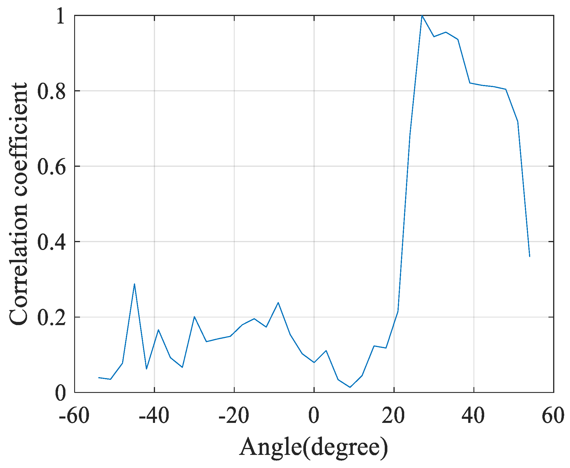
The spatial characteristics of directional noise were analyzed based on measured data. Then, a correlation analysis method based on angle-Doppler joint multi-eigenvector synthesis was proposed to analyze the spatial correlation of directional noise. The results demonstrated that directional noise has much higher correlation coefficients than omnidirectional noise. On this basis, an algorithm based on sliding main lobe cancellation (SL-MLC) for directional noise based on SSNSF was proposed, which could estimate directional noise more accurately under the condition of low spatial domain correlation;
In addition, compared to the standard MLC method, DBF, and JDL, the proposed algorithm could suppress directional noise more effectively, which met the requirements of the target detection threshold.
This paper is organized as follows. Firstly, the data model of the HFSWR system and the causes of directional noise generation have been introduced in
Section 2. In
Section 2.3, a correlation analysis method based on angle-Doppler joint multi-eigenvector synthesis is proposed to analyze the spatial correlation of directional noise. On this basis, the framework of SL-MLC is proposed, and the analyses of the impact of amplitude-phase errors are shown in
Section 3.
Section 4 describes the experimental results of the SL-MLC algorithm and presents an analysis of the results. Finally,
Section 5 gives the conclusion of this study.
3. Proposed Framework: SL-MLC
The MLC method is developed from the generalized side lobe canceler (GSC) proposed by Griffiths [
44] and is mainly applied to adaptive acoustic noise cancellation at first [
45]. With the development of ocean remote sensing technology, it is further applied to ionospheric clutter suppression, sea clutter suppression, and target detection of HFSWR. The principle of the MLC method is to use the blocking matrix to obtain target-free training data to estimate the covariance matrix of the noise or clutter. The ionospheric clutter and sea clutter in HFSWR have a strong correlation in the spatial dimension, so we can use the clutter information in other directions to estimate the main lobe direction to achieve clutter suppression.
There are also similar characteristics for direction noise in HFSWR. In addition, the training data used to estimate directional noise information cannot contain the target information to prevent target self-cancellation. Through previous studies, the blocking matrix is composed of a single-notch space filter (SNSF), which can achieve the separation of target and clutter. In the situation of a clutter hybrid with multiple targets, the system requires a large degree of freedom. To ensure that the system has enough freedom, an auxiliary channel is established by way of a sliding sub-array to obtain auxiliary data. However, directional noise has both the randomness property of noise and the directional distribution property of clutter, so how to estimate the directional noise more effectively and accurately based on its multiple properties is the key problem of directional noise elimination. To solve this problem, we propose an SL-MLC method that combines mathematical and statistical theories to achieve the suppression of directional noise. The main principle of the SL-MLC method is to design the blocking matrix according to the main lobe width and beam interval to achieve more accurate directional noise estimation.
3.1. Slide Single-Notch Space Filter
Through previous research, an SNSF is usually chosen as the blocking matrix using the least P-norm FIR filter to block the target information [
24]. However, the conventional SNSF method for estimating directional noise is not precise. As is known, the MLC method’s performance depends on the accuracy of the covariance matrix estimation of directional noise. To solve this problem, we proposed a directional noise suppression method based on SSNSF by utilizing multiple properties of directional noise. The structure diagram of SSNSF to achieve directional noise estimation is shown in
Figure 8.
SSNSF is a combination of the directional noise spatial characteristics, the spatial characteristics of the target, the configuration of the antenna array, and the structural characteristics of the SNSF itself. SSNSF is mainly considered in two aspects: first, the sliding parameters are designed according to the antenna array configuration and beam parameters; second, the SNSF filter is designed according to the information of the target parameters. Corresponding to different system operating frequencies, the SNSF can be obtained in different directions by the phase rotation method.
The responses of digital beam forming (DBF) and SSNSF are shown in
Figure 9 with the array elements
N = 16 and
= 10, and the main lobe direction is 2°. The entire spatial zone (from −90° to 90°) is divided into 91 beam cells (2° interval), and the main lobe width of the array is 12°. Hence, a single SNSF slides six times within the main lobe to form the SSNSF. However, the beam interval cannot be too small, which will lead to higher computational costs. So, in practice, the empirical beam interval is 3°. The SNSF slides within the width of the main lobe based on the beam spacing (red arrow pointing) in turn, and the red, blue, and green lines represent the SNSF at different sliding moments. The depth of the filter should be deeper than the target power to completely block the target component, and careful design of the SSNSF is required to ensure the filtering effect.
3.2. Signal Model of Directional Noise Excision
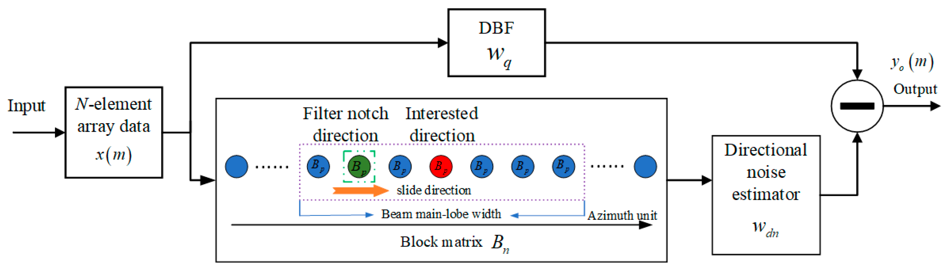
In the SL-MLC algorithm, the data is divided into two pathways. One main channel, which performs digital beamforming of the data by fixed static weighting, is the main lobe pointing in the direction of interest. The other is an auxiliary channel, which first filters out the signal components corresponding to the direction of the main lobe by SSNSF to ensure that the residual components do not contain the target component and prevent the target from self-canceling. Then the direction noise information obtained in the sidelobe is used to estimate the direction noise information of the main lobe. Finally, directional noise cancellation is realized by using the difference between the main channel data and the estimated directional noise information of the auxiliary channel. As shown in
Figure 10, the upper path has a fixed static weight
for digital beamforming to ensure beam direction and sidelobe level. The following path includes the blocking matrix B and the directional noise estimator.
As shown in the framework of the SL-MLC method in
Figure 10, the output can be indicated as:
where
denotes the static weights of the echo obtained by the receiving array, which are the coefficients of DBF in the desired direction. The blocking matrix
is used to block the target components to obtain training data, which is composed of SSNSF and
corresponds to different sliding moments.
is the adaptive weight vector calculated from the estimated directional noise covariance. Let
denote the cost function, and the optimal weight
can be obtained by solving the following unconstrained optimization problems:
where
is the self-correlation matrix,
. To keep the SNR loss minimized,
must only contain directional noise, excluding the target.
Hence, the optimal
can be calculated as:
The expression of signal to interference plus noise ratio (SINR) is as follows:
where
represents the power of the target and
denotes the average power of directional noise plus omnidirectional noise. In this paper, we take SINR as the evaluation index of algorithm performance.
3.3. Algorithm and Procedure Details
During data processing, firstly, digital beam formation (primary beam) and SSNSF auxiliary beam formation are performed on the channel domain data. The primary beam that extracts the distance to be processed and the auxiliary beam data output from the SSNSF constitute the primary and auxiliary channels, respectively. The main beam can use the Chebyshev weighted pattern to point in a specific direction of the beam to ensure sidelobe characteristics. SSNSF is a notch corresponding to the main beam pointing to a spatial blocking matrix. Define the output of the main channel as , the output of SSNSF as , and the result of directional noise cancellation as .
For adaptive estimation, the estimated accuracy of directional noise is better as the number of secondary data points is greater. In this case, we divide the receiving array into
sub-arrays by sliding
elements into each sub-array to obtain
SNSF outputs. First, we define an SNSF with the coefficients
as the block matrix
with the
-th sliding moments. Therefore, the block matrix
can be expressed as:
The output of the
i-th block matrix
with the
-th sliding moments is shown below:
Then, all the block matrix outputs from the data matrix
with the
-th sliding moments can be expressed as:
The total secondary
data can be written as follows:
The output of the
i-th DBF can be expressed as:
All the DBF outputs form the data vector
as expressed in Equation (22):
Adaptive optimal weight can be obtained by the minimum mean square error (MMSE), ideally.
Thus, the final output after directional noise cancellation can be expressed as:
Based on the above analysis and derivation, we present the detailed steps of SL-MLC in Algorithm 1 and the flowchart of the directional noise suppression procedure in
Figure 10.
| Algorithm 1 SL-MLC
|
Inputs: raw echo with directional noise;
Outputs: echo data with directional noise removed;
Initialization: |
| Set the number of sub-arrays , the block matrix coefficients , , , and the corresponding sliding moments ; |
- (1)
Calculate the i-th block matrix output with the -th sliding moments using Equation (16); - (2)
Calculate all the block matrix output of all the sub-arrays with the -th sliding moments using Equation (17); - (3)
Calculate the total secondary data of all the sliding moments using Equations (18) and (19); - (4)
Calculate the DBF outputs using Equations (20) and (22); - (5)
Calculate the self-correlation matrix and the cross-correlation matrix using Equations (24) and (25); - (6)
Calculate the final optimal weights for directional noise estimation using Equation (23); - (7)
Calculate the final output of SL-MLC using Equation (26); - (8)
Repeat steps (1) to (7) for processing the whole range units and beam units.
|
3.4. Analysis of Amplitude-Phase Error
There are some limitations to the SL-MLC method. In this section, we give an analysis of the amplitude-phase errors’ impact on the performance of the algorithm. The SL-MLC method utilizes the auxiliary data based on SSNSF to estimate the directional noise information, so the receiving antenna amplitude-phase error will seriously affect the performance of the algorithm. The amplitude error will change the level of the side lobe response, and the phase error will affect the depth and direction of the SNSF notch. In some extreme situations, the notch of SNSF may even disappear due to the heavy amplitude-phase errors, which will lead to the self-cancellation of the target and make the algorithm fail. Therefore, the compensation of amplitude and phase errors is essential in practical signal processing.
It is generally believed that the amplitude and phase error are quantities independent of the Direction of Arrival (DOA), which is expressed as a fixed error value in mathematical modeling. The modeling of amplitude-phase error is usually described by introducing an azimuth-independent amplitude-phase error vector into the steering vector:
where
denotes the amplitude and phase error coefficient,
and
denotes the amplitude and phase errors, respectively.
denotes the steering vector, and
indicates the steering vector with amplitude and phase error.
Here, we analyze the effects of amplitude error and phase error on the spatial response of SNSF to guide the algorithm to have better cancellation performance in the actual processing.
Figure 11a shows the ideal response and the response under different amplitude error scopes of SNSF, respectively. The amplitude errors are set to be uniformly distributed pseudorandom numbers in the [−1 1] dB, [−2 2] dB, and [−5 5] dB scopes.
Figure 11b shows the depth of the notch of the spatial response under different amplitude error scopes of SNSF under 1000 Monte Carlo simulations. The maximum amplitude error scopes are set to [0 10] dB with an interval of 0.1 dB. We can see from the results that the amplitude error will not only affect the side lobe response, causing the inequality of the side lobe response but also lead to a decrease in the depth of the notch of the spatial response. This will cause the main lobe information and side lobe information in the auxiliary channel to increase simultaneously, which is not conducive to the estimation of directional noise. At the same time, the reduction in the depth of the notch will cause the target component to be completely blocked, the target energy after suppression to be seriously reduced, and the signal-to-noise ratio to be lost, which is not conducive to the subsequent target detection.
Figure 11c shows the ideal response and the spatial response under different phase error scopes of SNSF, respectively. The phase errors are set to be uniformly distributed pseudorandom numbers in [−1 1] degree, [−3 3] degree, and [−6 6] degree scopes, representing different phase distortions. We can see that the phase error will lead to both a shift in the direction of the notch and a reduction in the depth of the notch. This will cause the target signal from the interested direction to be less suppressed by the filter, and the information of the target signal cannot be completely filtered out.
Figure 11d shows the depth of the notch of the spatial response under different phase error scopes of SNSF under 1000 Monte Carlo simulations. The maximum phase error scope is set to [0 10] degrees with an interval of 0.1 degrees. From the results, we can see that the phase error fluctuation will affect the depth of the notch, and in severe cases, it may even prevent the SNSF from acting as a spatial domain filter.
In conclusion, the amplitude and phase errors have a great impact on the notch depth, the side lobe response, and the notch direction of SNSF. Therefore, it is necessary to calibrate and compensate the array antenna before signal processing to ensure the consistency of the amplitude-phase.
4. Experimental Results
Directional noise elevates the noise base level. Weak targets will not be detected at the same detection threshold, seriously affecting the performance of the HFSWR system. Hence, in this section, we evaluate the validity and advantages of the proposed method by conducting exhaustive simulations and experimental studies based on measured data. These measured data are the same as the HFSWR data introduced in
Section 2.2. Meanwhile, the experimental results were compared with DBF, joint domain localized (JDL), and the conventional MLC algorithm. In the JDL, the size of the local process region is
; four is the number of Doppler cells; and five is the number of angular cells. In a conventional MLC, the number of sub-array elements is 10. For the SL-MLC method, the beam interval is 3° and
P is six. The simulated target with the detailed parameters in
Table 2 was injected into the directional noise region.
It should be noted that the initial purpose of directional noise suppression was to achieve the detection of specific target signals. Currently, the most widely used target detection method is the CFAR algorithm. In the practical HFSWR system, the CFAR method needs to meet a certain detection threshold to ensure a certain false alarm rate. Hence, to better test the performance of the proposed algorithm, the SINR of the simulated target we injected is lower than the detection threshold. In other words, the weak target masked by directional noise cannot be detected.
Figure 12a shows the angle-Doppler map obtained by the DBF method. As shown in the figure, the directional noise is widely distributed in the angle and Doppler domains, completely covering the simulated target information. The angle-Doppler map obtained by the SL-MLC method is demonstrated in
Figure 12b. Compared with the DBF method, it is obvious that the directional noise has been suppressed and targets submerged in the directional noise appear.
Figure 13 illustrates the results of the Doppler profile, which displays the directional noise suppression performance of the proposed algorithm. It can be seen from the results that the performance of SL-MLC is significantly better than the traditional MLC method. Compared with the JDL method, it also has certain performance improvements. However, since directional noise has no space-time characteristics, although the JDL method can suppress directional noise, it also appears to be a false target.
The SINR improvement, which indicates the improvement of the SINR after directional noise suppression, is introduced to quantitatively evaluate the performance of different algorithms. The expression of SINR improvement is as follows:
where SINR is calculated using Equation (13).
For HFSWR, it has a high Doppler frequency resolution, but the range resolution is relatively poor. Therefore, the Doppler profile is often used to show the performance of directional noise suppression. In this paper, the SINR improvement was calculated based on the Doppler profile. The average power of directional noise plus omnidirectional noise was calculated by several Doppler bins around the target, and the target power was calculated by the target’s Doppler bin.
The SINR improvement results are illustrated in
Table 3. For the simulated target, the proposed algorithm had the highest SINR improvement. The SINR improvements of DBF, JDL, MLC, and the proposed method are 0.55 dB, 3.45 dB, 1.67 dB, and 5.42 dB, respectively. After directional noise suppression, the SINR of DBF, MLC, JDL, and the proposed method are 11.55 dB, 12.67 dB, 14.45 dB, and 16.42 dB, respectively. In applications, it is generally considered that the SINR higher than the detection threshold is the target. In a practice radar system, the detection threshold is set to 14 dB according to the empirical value. In this case, only the JDL method and the proposed method are higher than the detection threshold. Thus, target detection can be easily realized. Fortunately, the SL-MLC proposed in this paper can suppress directional noise and improve SINR while protecting target information, which is a great advantage for detecting weak targets submerged by directional noise, such as aircraft targets moving at high speed. Although the method proposed in this paper has little improvement on SINR, it is of great help to improve the sensitivity of HFSWR. It plays an important role in improving the geographical environment adaptability, electromagnetic environment adaptability, and robustness of HFSWR.
Directional noise has both the random property of noise and the directional distribution property of clutter. The advantage of the SL-MLC method is that it can combine the multiple properties of directional noise to estimate it more accurately. To verify it, we conducted two sets of comparison experiments. Theoretically, the covariance matrix calculated by the blocking matrix without injecting the simulation target represents pure directional noise information. The covariance matrix calculated by the blocking matrix when injecting the simulation target represents the main lobe directional noise that needs to be canceled. Under the same experimental parameters, we use the estimated pure directional noise without injecting the simulated target to replace the estimated main lobe directional noise by injecting the simulated target. Then, the improvement of the target is used as the criterion to judge the accuracy of directional noise estimation. The experimental results are shown in
Figure 14. Compared with the MLC method, the target amplitude improved by 4.43 dB before and after the experiment. Hence, the performance of the SL-MLC algorithm is better than that of conventional MLC for directional noise estimation.
The SINR after signal processing of injected targets at different SINR values from 5 to 35 dB is shown in
Figure 15, which is used to evaluate the performance of the SL-MLC algorithm under different SINRs. The SINR after directional noise suppression by different methods is given by Monte Carlo simulations of 100 trials. The SINR was calculated based on the Doppler profile. In general, the SINR is increasing, with the SINR and magnitude of simulated targets increasing. Initially, when the SINR of the simulated target is very low (<9 dB), all the methods cannot achieve a better performance improvement, and the target cannot be detected. When the simulated targets’ magnitude and SINR are relatively large (9–35 dB), SL-MLC expects to uncover the covered targets earlier. Fortunately, the proposed algorithm is better than the comparison algorithm in terms of the overall trend. It is worth noting that when the SINR of the simulation target reaches 25 to 35 dB, the SINR obtained by the conventional MLC method and the DBF method is almost the same. This phenomenon can be attributed to the fact that the rising target amplitude and SINR cause the target energy to be leaked into the side-lobe, leading to target self-elimination. At the same time, the SINR obtained by the JDL method gradually approaches that obtained by the SL-MLC method.
In conclusion, compared with the DBF method, JDL method, and traditional MLC method, the SL-MLC method achieves a higher SINR improvement after applying directional noise suppression. Therefore, the proposed algorithm can assist in detecting targets with low SINR.


