Article

Time-Series-Based Spatiotemporal Fusion Network for Improving Crop Type Mapping

1
School of Resources and Environmental Engineering, Anhui University, Hefei 230601, China
2
CCCC Second Highway Consultants Co., Ltd., Wuhan 430056, China
3
Guangxi Zhuang Automomous Region Institute of Natural Resources Remote Sensing, Nanning 530023, China
4
School of Resources and Environment, Anhui Agricultural University, Hefei 230036, China
5
Information Materials and Intelligent Sensing Laboratory of Anhui Province, Anhui University, Hefei 230601, China
6
State Key Laboratory of Remote Sensing Science, Aerospace Information Research Institute, Chinese Academy of Sciences, Beijing 100101, China
*
Author to whom correspondence should be addressed.
Remote Sens. 2024, 16(2), 235; https://doi.org/10.3390/rs16020235
Submission received: 23 November 2023 / Revised: 30 December 2023 / Accepted: 4 January 2024 / Published: 7 January 2024
(This article belongs to the Special Issue Within-Season Agricultural Monitoring from Remotely Sensed Data)

Abstract

:
Crop mapping is vital in ensuring food production security and informing governmental decision-making. The satellite-normalized difference vegetation index (NDVI) obtained during periods of vigorous crop growth is important for crop species identification. Sentinel-2 images with spatial resolutions of 10, 20, and 60 m are widely used in crop mapping. However, the images obtained during periods of vigorous crop growth are often covered by clouds. In contrast, time-series moderate-resolution imaging spectrometer (MODIS) images can usually capture crop phenology but with coarse resolution. Therefore, a time-series-based spatiotemporal fusion network (TSSTFN) was designed to generate TSSTFN-NDVI during critical phenological periods for finer-scale crop mapping. This network leverages multi-temporal MODIS-Sentinel-2 NDVI pairs from previous years as a reference to enhance the precision of crop mapping. The long short-term memory module was used to acquire data about the time-series change pattern to achieve this. The UNet structure was employed to manage the spatial mapping relationship between MODIS and Sentinel-2 images. The time distribution of the image sequences in different years was inconsistent, and time alignment strategies were used to process the reference data. The results demonstrate that incorporating the predicted critical phenological period NDVI consistently yields better crop classification performance. Moreover, the predicted NDVI trained with time-consistent data achieved a higher classification accuracy than the predicted NDVI trained with the original NDVI.

1. Introduction

The spatial distribution of crop planting is critical for effective government decision-making, accurate estimation of crop yields, and efficient management of agricultural resources [1,2]. Traditional ground investigation methods are time-consuming and labor-intensive and cannot meet the needs of timely and large-scale monitoring. Remote sensing has the advantages of being fast, large-scale, and high-precision and has been proven to be an important data source for modern agricultural management. Remotely sensed crop mapping mostly uses spectral reflectance and phenological characteristics [3]. Remote sensing image reflectance data and the vegetation index during vigorous growth stages of crops can substantially enhance the accuracy of crop identification [4,5,6]. Meanwhile, compared with a single image, time-series images can provide more information about phenological changes and obtain higher recognition accuracy [4,7,8]. However, even using time-series images for classification, incorporating images during vigorous growth stages can still significantly improve the accuracy [4].
The normalized difference vegetation index (NDVI) [9] is an important parameter for crop growth monitoring. Remote sensing-derived NDVI time series is one of the most recognized methods in the field of crop mapping [10,11]. However, the spatiotemporal resolution of NDVI images largely determines the crop distribution information that can be extracted from it [12]. In most cases, there is a trade-off between the temporal and spatial resolutions of the same satellite sensor. In addition, adverse weather conditions, such as cloudy periods, limit the amount of available data. For instance, Sentinel-2, with its simultaneous dual-satellite observations, revisit period of up to five days, and multi-spectral data with a spatial resolution of up to 10 m, is widely applied in agriculture [13,14,15]. However, during periods of vigorous crop growth, there are often long spans of missing observations that seriously affect the effectiveness of crop classification [16,17]. Conversely, the high revisit frequency of the moderate-resolution imaging spectrometer (MODIS) approach enables the observation of rare cloud-free images during prolonged cloudy periods and provides crop information references for missing times. However, the coarse spatial resolution of MODIS imaging limits its application at a regional scale.
Spatiotemporal fusion methods can effectively address the issue of limited temporal and spatial resolutions in remote sensing imaging [18]. Existing spatiotemporal fusion algorithms can generally be divided into four categories: weight-function-based spatiotemporal fusion methods, learning-based methods, unmixing-based methods, and flexible methods [19,20]. The spatial and temporal adaptive reflectance fusion model (STARFM) [18] was a relatively early and notable model. Researchers have also explored the use of fused images for crop classification [21,22,23]. However, studies have mostly explored the effectiveness of existing traditional spatiotemporal fusion algorithms in crop classification. These fusion methods usually obtain only fused images and are rarely designed to improve crop classification accuracy. Yang et al. [24] used deep learning-based spatiotemporal fusion technology to optimize crop classification results automatically. However, they used the spatiotemporal fusion technology to fuse the classification results based on image blocks and pixels. Crops have certain phenological cycle characteristics. Therefore, the fusion of crop images should be considered using time-series data. A few scholars have fused time-series data and achieved high accuracies [19,25,26,27,28,29]. However, most of these studies manually designed time-change models, which resulted in the insufficient utilization of temporal information. A novel spatiotemporal fusion method that considers time-series data for crop classification is required.
In recent years, with the rise of artificial intelligence, recurrent neural networks (RNNs) are commonly used in land cover mapping due to their ability to capture temporal changes [30]. However, RNNs cannot capture long-term dependence. LSTM, as a variant of RNNs, effectively solves this problem by introducing gating mechanisms [31,32,33,34]. This study proposes a novel time-series-based spatiotemporal fusion network (TSSTFN) for crop classification that combines LSTM, UNet, and attention mechanisms to learn deep spatiotemporal features. LSTM captures time-series information, UNet extracts multi-level features in the spatial-spectral domain [35,36,37,38,39], and the attention mechanism allows the focus on key information while suppressing unnecessary information [40]. The aim is to develop a model to automatically capture the phenological cycle characteristics of different crops and discover the relationship between high- and low-resolution NDVI image pairs. The predicted high-resolution NDVI data of critical phenological periods in the required years can be applied to improve the accuracy of crop identification.
The remaining parts of this study have been divided into four parts. The materials and methods are introduced in the second section. The third section presents and analyzes the results of spatiotemporal fusion and crop mapping. The fourth section discusses the results obtained from other data processing strategies and the advantages and disadvantages of the model. Finally, the fifth section provides a summary.

2. Materials and Methods
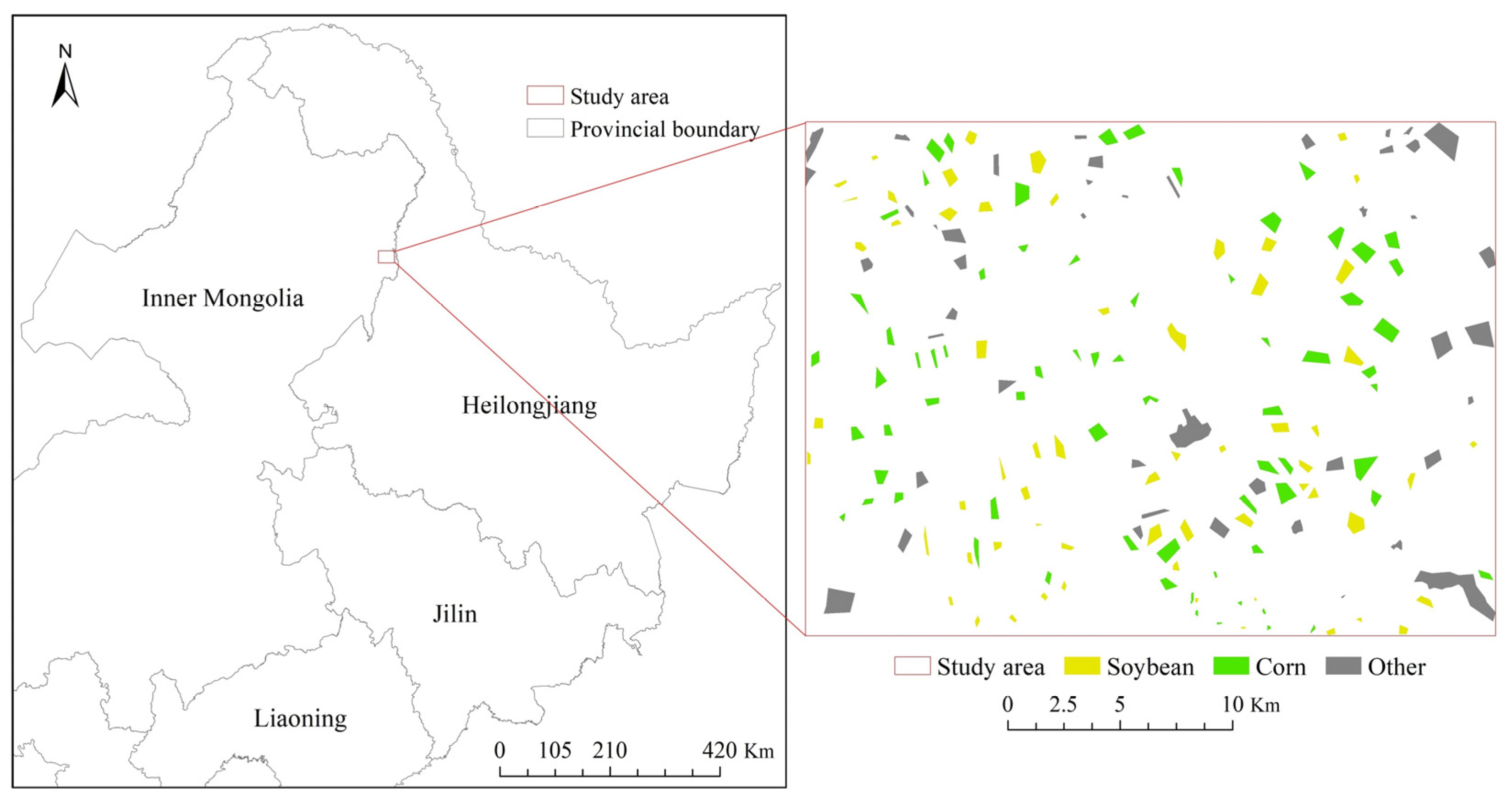
2.1. Study Area

The study area is located at the junction of Inner Mongolia and Heilongjiang in Northeast China (Figure 1). It covers an area of approximately 704 km2, equivalent to 3071 × 2294 Sentinel-2 pixels. The region experiences a temperate continental monsoon climate with four distinct seasons, with most of the precipitation occurring in July and August. The main crops are soybean and corn, typically planted in April, mature in August, and harvested in September and October. According to the crop phenology calendar (Figure 2) obtained from the official website of the Ministry of Agriculture and Rural Affairs of the People’s Republic of China (http://www.moa.gov.cn/, accessed on 8 June 2023), late July and August are the periods of vigorous growth for soybean and corn [41].
The NDVI time-series curves of crops can closely reflect the changes in crops in the whole process from growth to harvest. Accordingly, the NDVI time-series curves of soybean and corn in the study area were plotted using the time-series Sentinel-2 images in 2020. Due to the limited number of images, the Savizky–Golay filter [42] was used to smooth and reconstruct the NDVI time-series curve (Figure 3) [43]. As can be seen from the NDVI time-series curve, the growth cycles of soybean and corn are very similar, as are the NDVI values. The difference in NDVI values gradually increases after the emergence of crops in May, and the difference is relatively large in July and August. The difference in September and October is obvious because the crops gradually ripen and are harvested during this period. Delayed harvest will adversely affect the classification.

Data Preparation

The Sentinel-2 mission has two satellites, A and B, that operate simultaneously, allowing for relatively high temporal and spatial resolution. The revisit cycle can be as short as 5 days. The spatial resolution of the red and near-infrared bands is 10 m, which meets the requirements for crop mapping in the research area. The surface reflectance data from Sentinel-2 were primarily obtained and cropped from the Google Earth Engine platform (“COPERNICUS/S2_SR”).
The MOD09GQ Version 6.1 product provides daily observations of infrared and near-infrared bands with a spatial resolution of 250 m. All MOD09GQ products were downloaded from the United States National Aeronautics and Space Administration Level 1 and Atmosphere Archive and Distribution System Distributed Active Archive Center website (https://ladsweb.modaps.eosdis.nasa.gov/, accessed on 7 January 2023).
The dates of the selected cloud-free images are listed in Table 1. The 2020 data were primarily used for training, while the 2021 data were mainly used for testing and crop identification. Previous studies have shown that calculating NDVI first and then performing fusion yields better results than performing fusion first and then calculating NDVI [44,45,46]. Therefore, all subsequent fusion and crop mapping experiments were performed based on NDVI data.
The MODIS data were reprojected, cropped, and resampled using cubic interpolation to match the Sentinel-2 images. All images were cropped into 192 × 192 pixels before training and prediction. To increase the amount of training data, the adjacent sub-images were overlapped by half when cropping the training image. In the predicted image sequence, adjacent sub-images were overlapped by 10 pixels to ensure smooth blending of the results.
Reference and validation samples were produced using multi-period imagery from Sentinel-2. A total of 101,126 soybean sample points, 1,589,126 corn sample points, and 159,651 other samples were randomly selected, and the training and test samples were divided in a 7:3 ratio. The spatial distribution of the sampling points is shown in Figure 1.

2.2. Methods

As shown in Figure 4, the flowchart can be divided into two parts: spatiotemporal fusion and crop classification. In the first part, we processed and grouped the MODIS and Sentinel-2 NDVI pair sequences according to different training strategies, stacked the multiple base date MODIS-Seninel-2 NDVI pairs and the forecast date MODIS NDVI in chronological order as inputs, and used the TSSTFN to generate TSSTFN-NDVI during the critical phenological period of the required year. In the second part, we combined the above TSSTFN-NDVI and early Sentinel-2 NDVI sequences and crop classification samples, followed using accuracy evaluation and comparative analysis.

2.2.1. Fusion Model

As illustrated in Figure 5, the network architecture of the TSSTFN contains UNet, the convolutional block attention module (CBAM), and LSTM. UNet is the main structure that involves feature extraction through the encoder and feature fusion through the decoder. CBAM focuses on important features using channel and spatial attention modules. The LSTM component was inserted to process the time-series information and predict the value at a specific time.
The overall structure of the model is consistent with that of UNet. In the encoding structure, the number of filters in the convolutional block gradually increased from 64 to 1024, thereby deepening the level of the extracted features. Each convolutional block comprises two convolutional layers with a filter size of 3 × 3. Following each convolutional layer, batch normalization layer, dropout layer, and LeakyReLU activation functions were applied. The dropout layer randomly sets all elements of a channel in the input to zero, with a probability of 0.3. In addition, a pooling layer was inserted between the convolutional blocks to increase the receptive field. In the decoding structure, the output of the encoding structure was successively up-sampled to restore its size before entering the data-input network. To compensate for the loss of fine features, the up-sampled feature map was connected to the feature map extracted from the corresponding coding structure through the channel. These combined maps were then processed using convolution blocks with 512, 256, 128, and 64 filters based on their order in the decoding structure. Finally, the feature map produced using the decoding structure is passed through a convolutional layer with 3 × 3 filters to generate a TSSTFN-NDVI for the predicted date.
The CBAM was inserted after the first convolutional block. The channel attention module processes the results of global maximum pooling and global average pooling through a shared multi-layer perceptron, adds them, and generates the final channel attention map through the sigmoid activation function. The spatial attention module connects the maximum and average pooling results applied along the channel direction, convolutes them into a channel, and generates the final spatial attention map through the sigmoid activation function. The input of the CBAM was sequentially multiplied by the channel attention map and spatial attention map, and the product was added to the input of the CBAM to obtain the final output.
CBAM and LSTM were jointly applied (hereafter referred to as CL) for temporal change prediction at different spatial scales. The CL was inserted after the convolutional blocks with filter numbers 128, 256, and 512 (Figure 6). This module processes the same input through multiple identical CBAM modules, focuses on different features, and then processes them using LSTM. Because of the difference in data dimensions between the CNN and LSTM in the PyTorch framework, the last two dimensions must be flattened into one before inputting the data into the LSTM. Additionally, after adjusting the parameters, the input of each time step must be divided again, resulting in LSTM input feature numbers 384, 96, and 96, respectively, which can achieve higher accuracy. Therefore, the outputs of each LSTM must be sequentially connected to form a complete LSTM layer output. In this study, the input of the CL module was processed using CBAM and LSTM along these nine paths to obtain nine outputs. After channel connection, reshaping is required to maintain the dimensions and shape consistency of the last two dimensions with the input of the CL module.
The model was implemented using the PyTorch framework. During the training phase, we used the Adam optimizer with an initial learning rate of 0.001. To evaluate the performance of the model and prevent overfitting, we divided the training samples into training and validation sets at a ratio of 9:1. The validation set was used to monitor the overfitting. We employed an early stop strategy that involved recording the best accuracy achieved on the validation set during training. If the best accuracy did not surpass 12 consecutive epochs, the training process was terminated. The weights obtained at this point were considered the final parameters. The batch size was set to 16.

2.2.2. Crop Type Classification and Accuracy Assessment

The random forest (RF) classifier from the Scikit-learn library was used to identify crops. The parameters were determined through cross-validation [47,48,49]. Specifically, the number of trees (n_estimators), maximum depth of the tree (max_depth), and minimum number of training samples for the child nodes (min_samples_leaf) were set to 40, 25, and 20, respectively. To enhance the classification accuracy, we employed the multi-time-series value of the pixel being classified and the multi-time-series value of the 3 × 3 window centered on the pixel, as suggested by Sharma et al. [50].
The classification accuracy was evaluated using Cohen’s kappa coefficient, which assesses the consistency between the model’s and actual classification results. The kappa coefficient was calculated based on the confusion matrix using the following formula:
k a p p a = P 0 P e 1 + P e
where P0 is the number of correctly classified samples divided by the total number of samples, and Pe is the sum of the products of the actual samples and the predicted numbers corresponding to all categories divided by the square of the total number of samples.

2.2.3. Experiment Design

Two strategies were designed, STR_A and STR_B. For STR_A, we selected the satellite image sequences closest to the critical phenological periods in 2020 and 2021 for training and prediction, respectively. As shown in Figure 7, the two-year satellite image sequence times are inconsistent. Researchers usually use partially cloud-contaminated data directly to address this issue or find ways to fill in missing values [25,45,51,52]. Among them, the image-based temporal linear interpolation approach is undoubtedly the simplest and fastest. Therefore, we used temporal linear interpolation to obtain the 2020 interpolated images that were consistent with the 2021 time as STR_B. The STR_B image was obtained at a certain time by linear time interpolation of the satellite data before and after the time closest to the target time. Crop growth was the most vigorous and uniform in August, which is advantageous for feature classification. Therefore, in the training sequence, image selection for the critical phenological period was aligned with 31 August, regardless of whether we predicted the NDVI on 30 July, 31 August, or 5 September 2021. Many comparative experiments were performed based on early crop growth image data. The number of determined fused base image pairs was seven.
To illustrate the advantages of the proposed TSSTFN, an existing typical method (STARFM) was selected for comparison. STARFM requires one or two pairs of reference high- and low-resolution images and low-resolution images for predicting time. STARFM searches for similar pixels in a moving window from fine-resolution images and predicts the central pixels using the spatial, spectral, and temporally weighted mean differences of these similar pixels. Further details of this algorithm can be found in [18]. We chose 25 June 2021 as the reference date, which is the closest to the critical phenological period (i.e., 31 August 2021).
For crop mapping, it was assumed that no images would be available during the critical phenological periods in July and August 2021. Therefore, all available Sentinel-2 satellite NDVI sequences from April to June 2021 were used to identify crops. To prove the effectiveness of the TSSTFN, we added the predicted NDVI of the two strategies mentioned above to the NDVI sequence from April to June for crop identification.

3. Results

3.1. Assessment of the Spatiotemporal Fusion Results

To illustrate the effectiveness of the proposed method, the fused results were evaluated using visualization and quantitative metrics. Figure 8 shows the real Sentinel-2 NDVI on 31 August 2021, and NDVI fused in different ways. The fusion results of STARFM and TSSTFN with STR_A differed significantly from the actual Sentinel-2 NDVI, especially in the high NDVI region. In contrast, the fusion result of TSSTFN with STR_B was closer to the actual Sentinel-2 NDVI. The quantitative evaluation results (i.e., RMSE and SSIM) of the real Sentinel-2 NDVI and the fused NDVI are shown in Table 2. The quantitative evaluation results of the TSSTFN with STR_B were better than those of the TSSTFN with STR_A and STARFM. In addition, the TSSTFN scores with STR_A were slightly inferior to those with STARFM. These findings indicate the necessity of time alignment between the training and testing sequences for the TSSTFN.

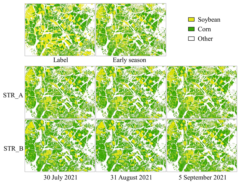
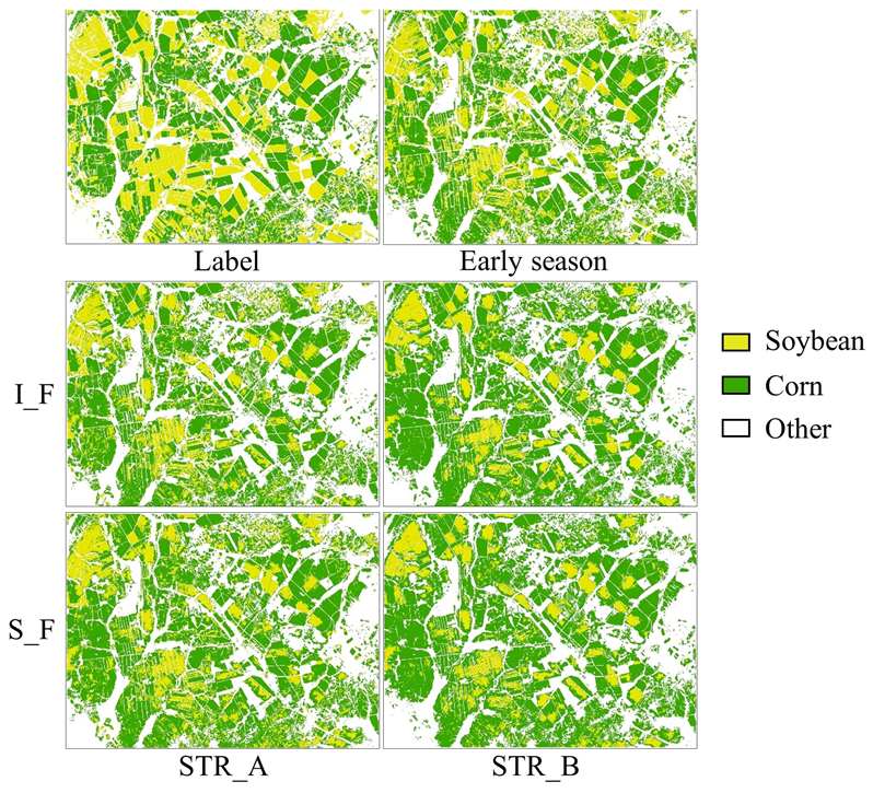
3.2. Crop Maps with Addition of One Prediction in the Critical Phenological Period

In addition to the images from the early season, the crop maps generated by separately incorporating TSSTFN-NDVI on 30 July, 31 August, and 5 September 2021 are shown in Figure 9. Although the adopted RF classification method can discriminate crops from non-crops very well, accurately distinguishing between soybeans and corn using only the satellite NDVI from April to June (early season) has proven difficult, resulting in many misclassifications. This situation improved when fused data were added to the data source during the early seasons. Overall, compared with the crop map from early reasons (i.e., without fused data), the crop maps with fused data from both STR_A and STR_B were closer to the label. In addition, the crop maps with fused data from STR_B showed better visual effects than those from STR_A. Interestingly, the crop maps with the fused TSSTFN-NDVI on 5 September 2021 seemed slightly inferior to those on 30 July and 31 August 2021. The most probable cause is that on 5 September, the critical phenological period had already passed and was the farthest from the base dates. Except for the label, it is worth noting that the generated crop maps have a certain degree of fragmentation. The similar growth cycles and spectra of soybean and corn make crop classification more challenging and cause further fragmentation. Additionally, inconsistencies in the growth of crops in different fields, or even in the same field, may result in mapping errors.
The values of the kappa coefficients are listed in Table 3 to quantitatively compare the mapping accuracies of the crop maps in Figure 9. The kappa coefficient of the crop map from the early reason (i.e., without fused data) was 69.2%. This value was lower than that from both STR_A and STR_B at different dates. Moreover, the kappa coefficients for STR_B on 30 July, 31 August, and 5 September were 82.44%, 81.95%, and 74.22%, respectively. These values were higher than those for STR_A (3.94%, 74.84%, and 69.48%, respectively). Overall, crop maps with the addition of one prediction from STR_B on 30 July 2021 showed the highest classification accuracy, whereas crop maps from early reasons (i.e., without fused data) showed the lowest classification accuracy. The results show that adding fused NDVI during the critical phenological period can greatly enhance the accuracy of crop mapping, and time alignment between training and testing sequences (STR_B) for the TSSTFN can achieve higher classification accuracy.

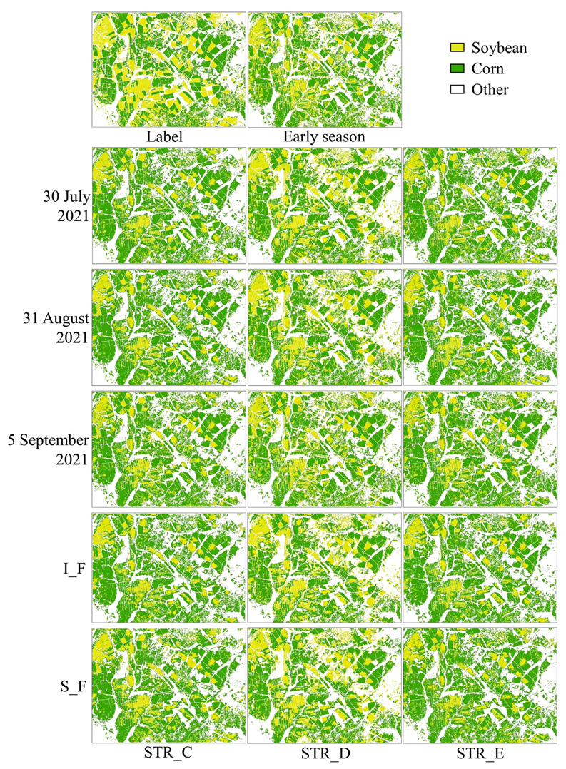
3.3. Crop Maps with Addition of Two Predictions in the Critical Phenological Period

We tested the performance of the crop maps with the addition of two predictions. The predictions of 30 July and 30 August were used together with the data of the early season (Figure 10). Notably, the prediction for 31 August can be fused in two ways: obtained only from the early original NDVI (Individual Forecast, I_F) and obtained from the early NDVI and fused NDVI on 30 July (Sequential Forecast, S_F). From a visual perspective, there was no obvious difference in the crop maps between I_F and S_F, whereas the effect of adding fused NDVI via STR_B was better than that via STR_A for both I_F and S_F. However, adding one prediction in the critical phenological period resulted in crop maps with fused data from both I_F and S_F in different strategies (STR_A and STR_B) with higher accuracy than maps without fused data.
Table 4 presents the quantitative evaluation results of the kappa coefficient, which directly correspond to the crop maps in Figure 10. The addition of two predictions was better than the addition of only one prediction. For STR_A, individual predictions improved relatively, whereas for STR_B, sequential predictions improved relatively.

4. Discussion

4.1. Other Strategies

In the spatiotemporal fusion strategy, training data can be temporally linearly interpolated to make their time series consistent with the predicted data. The predicted data can be temporally linearly interpolated to make their time series consistent with the training data. Simultaneously, the training and prediction data were interpolated to correspond to each other (STR_C). In addition, data with missing times can be replaced with the closest data in time. These alternative methods can be divided into STR_D and STR_E based on whether they are used for training data or both training and prediction data. The specific strategies are illustrated in Figure 11.
The classification results obtained by adding the predicted NDVI via STR_C, STR_D, and STR_E to the early season NDVI sequence are shown in Figure 12, and the quantitative evaluation results are listed in Table 5. Overall, the addition of one or two predicted NDVI, STR_C, had a higher and more stable improvement in classification accuracy compared to STR_D and STR_E. Sequential forecasting had a significant additive effect on STR_C, directly increasing the kappa coefficient from 82.65% to 85.30%.
The kappa coefficients obtained from all fusion data strategies are displayed in a bar chart in Figure 13. All five strategies improved the classification accuracy. Among them, STR_A showed the smallest improvement, followed by STR_E. STR_B, STR_C, and STR_D were more accurate and more stable. In most cases, the addition of two predictions was better than using the addition of one. Based on the data from five strategies, the end of June and early July are the stages of rapid changes in crop growth curves. STR_A and STR_E corresponded to the data from the end of June 2021 and early July 2020 in time, resulting in a relatively low improvement. STR_C had slightly higher accuracy than STR_B on 30 July and 31 August 2021, while the opposite was evident on 5 September. From the training and prediction data, it can be seen that the time-series data for STR_C started as early as May, while STR_B started as early as April. This may be because the data for May and June were more similar to the data for July and August, and the data for April were more similar to the data for September. STR_D was higher than STR_B and STR_C on 30 July and lower than STR_B and STR_C on 31 August and 5 September. This is because STR_D used data from 19 August 2020 to correspond to data from 2021, while STR_B and STR_C used interpolated data from 19 August and 10 September 2020. It is obvious that the data on 19 August 2020 are closer to the data on 30 July 2021, and the interpolated data are closer to the data on 31 August and 5 September 2021. In general, during the vigorous growth stages of crops, it is more appropriate to choose STR_D if the corresponding reference image time is later than the predicted time and STR_C if the corresponding reference image time is earlier than the predicted time. For STR_C, the sequential forecast is more suitable than the individual forecast, while STR_D is the opposite. This should also be because the selection of data for the peak growth period of crops in 2021 is different.

4.2. Advantages and Disadvantages of the Model

TSSTFN combines UNet, LSTM, and CBAM to achieve the spatiotemporal fusion of MODIS and Sentinel-2 NDVI. The main objective was to enhance the accuracy of crop identification by incorporating high spatial resolution NDVI data from critical phenological periods of crops into the early NDVI data. Traditional spatiotemporal fusion models require the design of time-series models when using multiple pairs of time-series images. These models rely on the number of reference image pairs and relatively simple change patterns [25]. Additionally, existing methods cannot utilize information from previous years’ data and usually only allow the use of data with a consistent crop distribution within a single year. In contrast, TSSTFN has two advantages. Firstly, it can learn the temporal variation of ground features from the data pairs of previous years with cloudless NDVI data during critical phenological periods of the crops, even when the crop types in the area remain unchanged, or crop rotation is adopted. Secondly, it allows for the timely generation of NDVI data for critical phenological periods, using early reference data pairs and low-resolution NDVI data from critical phenological periods that are rarely captured. Although the time inconsistency between the data series from the previous year and the current year poses some challenges to the fusion process, the four data strategies proposed in this study have been experimentally proven to effectively improve the accuracy of crop identification. Although there may be a network structure that is more suitable for multi-time-series spatiotemporal fusion to further enhance crop classification, the experimental results of this study demonstrate that TSSTFN can generate fusion NDVI data for critical phenological periods in a timely manner during the crop growth period, thereby improving crop mapping accuracy. Due to the similarity in growth cycle and spectrum, it is difficult to distinguish between corn and soybean [41]. The accuracy we have achieved in mapping corn and soybeans is sufficient to demonstrate the superiority of TSSTFN.
However, this method assumes that the crop species in the area remain the same and that high-resolution images are available from previous years for the critical phenological period. Before using this method, the crop phenology of the area must be analyzed to distinguish the critical phenological period. In addition, this model requires more input data pairs and involves several preprocessing tasks. Notably, this study specifically focused on the fusion of NDVI data, considering the relatively stable pattern of vegetation growth and the unique characteristics of NDVI. Therefore, whether it is suitable for other vegetation indices or reflectance data requires further investigation.

5. Conclusions

This study proposes a novel time-series NDVI spatiotemporal fusion model, TSSTFN, to discover the phenological patterns and correspondences between high- and low-resolution data. The goal was to improve crop classification accuracy in a timely manner using the fused TSSTFN-NDVI of the critical phenological period. The issue of inconsistent data times between different years of the original satellite data prompted the design of four additional data strategies to process the fused data. Adding the TSSTFN-NDVI of the critical phenological period to the NDVI sequence of the early season improved the crop classification accuracy. Furthermore, time alignment strategies improved the accuracy more significantly. This study demonstrates the potential of deep learning in the spatiotemporal fusion of NDVI sequences for crop classification.

Author Contributions

Conceptualization, Y.W. (Yongchuang Wu), Y.W. (Yanlan Wu), and P.W.; data curation, W.Z. and H.L.; formal analysis, W.Z., F.L., and J.L.; funding acquisition, H.L. and P.W.; investigation, W.Z. and J.L.; methodology, W.Z. and P.W.; project administration, W.Z.; resources, F.L. and Y.W. (Yanlan Wu); software, W.Z., Y.W. (Yongchuang Wu), and Z.Y.; supervision, Z.Y., Y.W. (Yanlan Wu), and P.W.; validation, W.Z.; visualization, W.Z. and Y.W. (Yongchuang Wu); writing—original draft, W.Z.; writing—review and editing, H.L. and P.W. All authors have read and agreed to the published version of the manuscript.

Funding

This work was partially funded by the Open Fund of State Key Laboratory of Remote Sensing Science (grant number OFSLRSS202205), the National Natural Science Foundation of China (grant number 42001331), the Key Natural Science Research Project of Higher Education Institutions in Anhui Province (grant number 2023AH051013), and the Anhui Provincial Natural Science Foundation (grant number 2308085Y29).

Data Availability Statement

The data presented in this study are available upon request from the corresponding author. The data are not publicly available due to permissions issues.

Conflicts of Interest

Author Feng Luo was employed by the company CCCC Second Highway Consultants Co., Ltd. The remaining authors declare that the research was conducted in the absence of any commercial or financial relationships that could be construed as a potential conflict of interest.

References

  1. Thenkabail, P.S.; Knox, J.W.; Ozdogan, M.; Gumma, M.K.; Congalton, R.G.; Wu, Z.; Milesi, C.; Finkral, A.; Marshall, M.; Mariotto, I.; et al. Assessing future risks to agricultural productivity, water resources and food security: How can remote sensing help? Photogramm. Eng. Remote Sens. 2012, 78, 773–782. [Google Scholar]
  2. Foley, J.A.; Ramankutty, N.; Brauman, K.A.; Cassidy, E.S.; Gerber, J.S.; Johnston, M.; Mueller, N.D.; O’Connell, C.; Ray, D.K.; West, P.C.; et al. Solutions for a Cultivated Planet. Nature 2011, 478, 337–342. [Google Scholar] [CrossRef]
  3. Zhong, L.; Gong, P.; Biging, G.S. Efficient corn and soybean mapping with temporal extendability: A multi-year experiment using Landsat imagery. Remote Sens. Environ. 2014, 140, 1–13. [Google Scholar] [CrossRef]
  4. Jiang, D.; Chen, S.; Useya, J.; Cao, L.; Lu, T. Crop Mapping Using the Historical Crop Data Layer and Deep Neural Networks: A Case Study in Jilin Province, China. Sensors 2022, 22, 5853. [Google Scholar] [CrossRef]
  5. Xu, M.; Jia, X.; Pickering, M. Cloud effects removal via sparse representation. In Proceedings of the 2015 IEEE International Geoscience and Remote Sensing Symposium (IGARSS), Milan, Italy, 26–31 July 2015; pp. 605–608. [Google Scholar] [CrossRef]
  6. Maponya, M.G.; Niekerk, A.V.; Mashimbye, Z.E. Pre-harvest classification of crop types using a Sentinel-2 time-series and machine learning. Comput. Electron. Agr. 2020, 169, 105164. [Google Scholar] [CrossRef]
  7. Xu, J.; Zhu, Y.; Zhong, R.; Lin, Z.; Xu, J.; Jiang, H.; Huang, J.; Li, H.; Lin, T. DeepCropMapping: A multi-temporal deep learning approach with improved spatial generalizability for dynamic corn and soybean mapping. Remote Sens. Environ. 2020, 247, 111946. [Google Scholar] [CrossRef]
  8. Hunt, E.R.; Daughtry, C.S.T. What good are unmanned aircraft systems for agricultural remote sensing and precision agriculture? Int. J. Remote Sens. 2018, 39, 5345–5376. [Google Scholar] [CrossRef]
  9. Rouse, J.W.; Haas, R.H.; Schell, J.A.; Deering, D.W. Monitoring Vegetation Systems in the Great Plains with ERTS; NASA Special Publication: Washington, DC, USA, 1974; p. 351. [Google Scholar]
  10. Werner, J.P.S.; Oliveira, S.R.D.; Esquerdo, J.C.D.M. Mapping Cotton Fields Using Data Mining and MODIS Time-series. Int. J. Remote Sens. 2020, 41, 2457–2476. [Google Scholar] [CrossRef]
  11. Crusiol, L.G.T.; Sun, L.; Chen, R.; Sun, Z.; Zhang, D.; Chen, Z.; Deji, W.; Nanni, M.R.; Nepomuceno, A.L.; Farias, J.R.B. Assessing the potential of using high spatial resolution daily NDVI-time-series from planet CubeSat images for crop monitoring. Int. J. Remote Sens. 2021, 42, 7114–7142. [Google Scholar] [CrossRef]
  12. Zhang, X.; Wang, J.; Henebry, G.M.; Gao, F. Development and evaluation of a new algorithm for detecting 30 M land surface phenology from VIIRS and HLS time series. ISPRS J. Photogramm. Remote Sens. 2020, 161, 37–51. [Google Scholar] [CrossRef]
  13. Song, X.; Huang, W.; Hansen, M.C.; Potapov, P. An evaluation of Landsat, Sentinel-2, Sentinel-1 and MODIS data for crop type mapping. Sci. Remote Sens. 2021, 3, 100018. [Google Scholar] [CrossRef]
  14. Tran, K.H.; Zhang, H.K.; McMaine, J.T.; Zhang, X.; Luo, D. 10 m crop type mapping using Sentinel-2 reflectance and 30 m cropland data layer product. Int. J. Appl. Earth Obs. Geoinf. 2022, 107, 102692. [Google Scholar] [CrossRef]
  15. Yang, C.; Suh, C.P.C. Applying machine learning classifiers to Sentinel-2 imagery for early identification of cotton fields to advance boll weevil eradication. Comput. Electron. Agr. 2023, 213, 108268. [Google Scholar] [CrossRef]
  16. Johnson, D.M.; Mueller, R. Pre- and within-season crop type classification trained with archival land cover information. Remote Sens. Environ. 2021, 264, 112576. [Google Scholar] [CrossRef]
  17. Vuolo, F.; Neuwirth, M.; Immitzer, M.; Atzberger, C.; Ng, W.T. How much does multi-temporal Sentinel-2 data improve crop type classification? Int. J. Appl. Earth Obs. Geoinf. 2018, 72, 122–130. [Google Scholar] [CrossRef]
  18. Gao, F.; Masek, J.; Schwaller, M.; Hall, F. On the blending of the Landsat and MODIS surface reflectance: Predicting daily Landsat surface reflectance. IEEE Trans. Geosci. Remote Sens. 2006, 44, 2207–2218. [Google Scholar] [CrossRef]
  19. Chen, S.; Wang, J.; Gong, P. ROBOT: A spatiotemporal fusion model toward seamless data cube for global remote sensing applications. Remote Sens. Environ. 2023, 294, 113616. [Google Scholar] [CrossRef]
  20. Ghamisi, P.; Rasti, B.; Yokoya, N.; Wang, Q.; Hofle, B.; Bruzzone, L.; Bovolo, F.; Chi, M.; Anders, K.; Gloaguen, R.; et al. Multisource and multitemporal data fusion in remote sensing: A comprehensive review of the state of the art. IEEE Geosci. Remote Sens. Mag. 2019, 7, 6–39. [Google Scholar] [CrossRef]
  21. Zhu, L.; Radeloff, V.C.; Ives, A.R. Improving the mapping of crop types in the Midwestern U.S. by fusing Landsat and MODIS satellite data. Int. J. Appl. Earth Obs. Geoinf. 2017, 58, 1–11. [Google Scholar] [CrossRef]
  22. Onojeghuo, A.O.; Blackburn, G.A.; Wang, Q.; Atkinson, P.M.; Kindred, D.; Miao, Y. Rice crop phenology mapping at high spatial and temporal resolution using downscaled MODIS time-series. GIScience Remote Sens. 2018, 55, 659–677. [Google Scholar] [CrossRef]
  23. Yin, Q.; Liu, M.; Cheng, J.; Ke, Y.; Chen, X. Mapping paddy rice planting area in northeastern China using spatiotemporal data fusion and phenology-based method. Remote Sens. 2019, 11, 1699. [Google Scholar] [CrossRef]
  24. Yang, S.; Gu, L.; Li, X.; Gao, F.; Jiang, T. Fully Automated Classification Method for Crops Based on Spatiotemporal Deep-Learning Fusion Technology. IEEE Trans. Geosci. Remote Sens. 2022, 60, 5405016. [Google Scholar] [CrossRef]
  25. Chen, Y.; Cao, R.; Chen, J.; Liu, L.; Matsushita, B. A practical approach to reconstruct high-quality Landsat NDVI time-series data by gap filling and the Savitzky–Golay filter. ISPRS J. Photogramm. Remote Sens. 2021, 180, 174–190. [Google Scholar] [CrossRef]
  26. Cao, R.; Xu, Z.; Chen, Y.; Chen, J.; Shen, M. Reconstructing high-spatiotemporal-resolution (30 m and 8-days) NDVI time-series data for the Qinghai–Tibetan Plateau from 2000–2020. Remote Sens. 2022, 14, 3648. [Google Scholar] [CrossRef]
  27. Guo, D.; Shi, W.; Hao, M.; Zhu, X. FSDAF 2.0: Improving the performance of retrieving land cover changes and preserving spatial details. Remote Sens. Environ. 2020, 248, 111973. [Google Scholar] [CrossRef]
  28. Wang, Q.; Tang, Y.; Tong, X.; Atkinson, P.M. Virtual image pair-based spatio-temporal fusion. Remote Sens. Environ. 2020, 249, 112009. [Google Scholar] [CrossRef]
  29. Sun, L.; Gao, F.; Xie, D.; Anderson, M.; Chen, R.; Yang, Y.; Yang, Y.; Chen, Z. Reconstructing daily 30 m NDVI over complex agricultural landscapes using a crop reference curve approach. Remote Sens. Environ. 2020, 253, 112156. [Google Scholar] [CrossRef]
  30. Mou, L.; Bruzzone, L.; Zhu, X. Learning spectral-spatial-temporal features via a recurrent convolutional neural network for change detection in multispectral imagery. IEEE Trans. Geosci. Remote Sens. 2019, 57, 924–935. [Google Scholar] [CrossRef]
  31. Yaramasu, R.; Bandaru, V.; Pnvr, K. Pre-season crop type mapping using deep neural networks. Comput. Electron. Agr. 2020, 176, 105664. [Google Scholar] [CrossRef]
  32. Jia, X.; Khandelwal, A.; Nayak, G.; Gerber, J.; Carlson, K.; West, P.; Kumar, V. Incremental dual-memory LSTM in land cover prediction. In Proceedings of the 23rd ACM SIGKDD International Conference on Knowledge Discovery and Data Mining 2017, Halifax, NS, Canada, 13–17 August 2017; pp. 867–876. [Google Scholar] [CrossRef]
  33. Rußwurm, M.; Körner, M. Temporal Vegetation Modelling Using Long Short-Term Memory Networks for Crop Identification from Medium-Resolution Multi-spectral Satellite Images. In Proceedings of the 2017 IEEE Conference on Computer Vision and Pattern Recognition Workshops (CVPRW), Honolulu, HI, USA, 21–26 July 2017; pp. 1496–1504. [Google Scholar] [CrossRef]
  34. Zhong, L.; Hu, L.; Zhou, H. Deep learning based multi-temporal crop classification. Remote Sens. Environ. 2019, 221, 430–443. [Google Scholar] [CrossRef]
  35. Huang, B.; Zhao, B.; Song, Y. Urban land-use mapping using a deep convolutional neural network with high spatial resolution multispectral remote sensing imagery. Remote Sens. Environ. 2018, 214, 73–86. [Google Scholar] [CrossRef]
  36. Chen, Y.; Shi, K.; Ge, Y.; Zhou, Y. Spatiotemporal Remote Sensing Image Fusion Using Multiscale Two-Stream Convolutional Neural Networks. IEEE Trans. Geosci. Remote Sens. 2022, 6, 100062. [Google Scholar] [CrossRef]
  37. Tan, Z.; Yue, P.; Di, L.; Tang, J. Deriving high spatiotemporal remote sensing images using deep convolutional network. Remote Sens. 2018, 10, 1066. [Google Scholar] [CrossRef]
  38. Song, H.; Liu, Q.; Wang, G.; Hang, R.; Huang, B. Spatiotemporal satellite image fusion using deep convolutional neural networks. IEEE J. Sel. Top. Appl. Earth Observ. Remote Sens. 2018, 11, 821–829. [Google Scholar] [CrossRef]
  39. Song, B.; Liu, P.; Li, J.; Wang, L.; Zhang, L.; He, G.; Chen, L.; Liu, J. MLFF-GAN: A multilevel feature fusion with GAN for spatiotemporal remote sensing images. IEEE Trans. Geosci. Remote Sens. 2022, 60, 4410816. [Google Scholar] [CrossRef]
  40. Chaudhari, S.; Mithal, V.; Polatkan, G.; Ramanath, R. An Attentive Survey of Attention Models. ACM Trans. Intell. Syst. Technol. 2021, 12, 1–32. [Google Scholar] [CrossRef]
  41. Wu, Y.; Wu, P.; Wu, Y.; Yang, H.; Wang, B. Remote Sensing Crop Recognition by Coupling Phenological Features and Off-Center Bayesian Deep Learning. Remote Sens. 2023, 15, 674. [Google Scholar] [CrossRef]
  42. Savitzky, A.; Golay, M.J.E. Smoothing and Differentiation of Data by Simplified Least Squares Procedures. Anal. Chem. 1964, 36, 1627–1639. [Google Scholar] [CrossRef]
  43. Chen, J.; Jönsson, P.; Tamura, M.; Gu, Z.; Matsushita, B.; Eklundh, L. A simple method for reconstructing a high-quality NDVI time-series data set based on the Savitzky-Golay filter. Remote Sens. Environ. 2004, 91, 332–344. [Google Scholar] [CrossRef]
  44. Chen, X.; Liu, M.; Zhu, X.; Chen, J.; Zhong, Y.; Cao, X. “blend-then-index” or “index-then-blend”: A theoretical analysis for generating high-resolution NDVI time series by STARFM. Photogramm. Eng. Remote. Sens. 2018, 84, 66–74. [Google Scholar] [CrossRef]
  45. Jarihani, A.A.; McVicar, T.R.; Van Niel, T.G.; Emelyanova, I.V.; Callow, J.N.; Johansen, K. Blending Landsat and MODIS data to generate multispectral indices: A comparison of “index-then-blend” and “blend-then-index” approaches. Remote Sens. 2014, 6, 9213–9238. [Google Scholar] [CrossRef]
  46. Liu, M.; Yang, W.; Zhu, X.; Chen, J.; Chen, X.; Yang, L.; Helmer, E.H. An Improved Flexible Spatiotemporal Data Fusion (IFSDAF) Method for Producing High Spatiotemporal Resolution Normalized Difference Vegetation Index Time Series. Remote Sens. Environ. 2019, 227, 74–89. [Google Scholar] [CrossRef]
  47. Nguyen, L.H.; Joshi, D.R.; Clay, D.E.; Henebry, G.M. Characterizing land cover/land use from multiple years of Landsat and MODIS time series: A novel approach using land surface phenology modeling and random forest classifier. Remote Sens. Environ. 2020, 238, 111017. [Google Scholar] [CrossRef]
  48. Tatsumi, K.; Yamashiki, Y.; Torres, M.A.C.; Taipe, C.L.R. Crop classification of upland fields using random forest of time-series Landsat 7 ETM+ data. Comput. Electron. Agr. 2015, 115, 171–179. [Google Scholar] [CrossRef]
  49. Gao, Z.; Guo, D.; Ryu, D.W.; Western, A. Training sample selection for robust multi-year within-season crop classification using machine learning. Comput. Electron. Agr. 2023, 210, 107927. [Google Scholar] [CrossRef]
  50. Sharma, A.; Liu, X.; Yang, X. Land cover classification from multi-temporal, multi-spectral remotely sensed imagery using patch-based recurrent neural networks. Neural Netw. 2018, 105, 346–355. [Google Scholar] [CrossRef]
  51. Luo, Y.; Guan, K.; Peng, J. STAIR: A generic and fully-automated method to fuse multiple sources of optical satellite data to generate a high-resolution, daily and cloud-/gap-free surface reflectance product. Remote Sens. Environ. 2018, 214, 87–99. [Google Scholar] [CrossRef]
  52. Yan, L.; Roy, D.P. Spatially and temporally complete Landsat reflectance time series modelling: The fill-and-fit approach. Remote Sens. Environ. 2020, 241, 111718. [Google Scholar] [CrossRef]
Figure 1. Study area and distribution of samples. Yellow indicates soybeans, green indicates corn, and grey indicates other.
Remotesensing 16 00235 g001
Figure 2. Crop phenology calendar in the study area. E, M, and L represent the first, middle, and last ten days of a month, respectively.
Remotesensing 16 00235 g002
Figure 3. NDVI time-series curves of soybean and corn in the study area filtered by the Savizky–Golay filter. Yellow indicates soybeans; green indicates corn.
Remotesensing 16 00235 g003
Figure 4. Flowchart of increasing data sources for crop identification using spatiotemporal fusion.
Remotesensing 16 00235 g004
Figure 5. TSSTFN architecture.
Remotesensing 16 00235 g005
Figure 6. CL architecture.
Remotesensing 16 00235 g006
Figure 7. Training data and prediction data schemes, taking 31 August 2021 as an example. The 2020 data were used for training, and the 2021 data were used for testing.
Remotesensing 16 00235 g007
Figure 8. Comparison between the real Sentinel-2 NDVI and the fused NDVI in different ways on 31 August 2021. The first row displays the real Sentinel-2 NDVI and the fusion results of STARFM, respectively. The second row displays the fusion results of TSSTFN with the STR_A and STR_B, respectively.
Remotesensing 16 00235 g008
Figure 9. Crop maps from adding one prediction using STR_A and STR_B on 30 July, 31 August, and 5 September, respectively. The label and the crop map using only Sentinel-2 extracted NDVI from the early season are used for comparison. The early season stands for classification using only Sentinel-2 extracted NDVI from April to June 2021.
Remotesensing 16 00235 g009
Figure 10. Crop maps from adding two predictions on 30 July and 31 August 2021 together. The label and crop map using only Sentinel-2 extracted NDVI from the early season are used for comparison. The early season stands for classification using only Sentinel-2 extracted NDVI from April to June 2021. I_F represents individual forecasts, and S_F represents sequential forecasts.
Remotesensing 16 00235 g010
Figure 11. Other training data and prediction data schemes, taking 31 August 2021 as an example. Data in 2020 were used for training and data in 2021 for testing.
Remotesensing 16 00235 g011
Figure 12. Crop maps from adding one or two predictions using STR_C, STR_D, and STR_E. Label and crop maps using only Sentinel-2 extracted NDVI from the early season are used for comparison. The early season stands for classification using only Sentinel-2 extracted NDVI from April to June 2021. I_F represents individual forecasts, while S_F represents sequential forecasts.
Remotesensing 16 00235 g012
Figure 13. Accuracy histogram for classification using only early NDVI and incorporating one or two predictions using all five strategies. The early season stands for classification using only Sentinel-2 extracted NDVI from April to June 2021.
Remotesensing 16 00235 g013
Table 1. Image date information.
Year Date
2020Training data18 April, 28 April, 6 May, 8 May, 18 May, 28 May, 7 July, 12 July, 15 July, 19 August, and 10 September.
2021Testing base date and classification data6 April, 8 April, 18 April, 21 April, 16 May, 21 May, 2 June, 12 June, 22 June, and 25 June.
Validate the predictions30 July, 31 August, and 5 September.
Table 2. Quantitative evaluation of fused NDVI in different ways on 31 August 2021.
STARFMSTR_ASTR_B
RMSE0.23570.28500.1274
SSIM0.99440.98990.9984
Table 3. Kappa coefficients for crop classification using with and without fusion data.
without Fusion Datawith Fusion Data
STR_ASTR_B
Early season 169.20
30 July 2021 73.9482.44
31 August 2021 74.8481.95
5 September 2021 69.4874.22
Results are expressed as %. 1 The early season stands for classification using only Sentinel-2 extracted NDVI from April to June 2021.
Table 4. Kappa coefficient for classification by incorporating two predictions on 30 July and 31 August 2021 together.
STR_ASTR_B
Individual forecast74.6484.07
Sequential forecast78.1582.53
Results are expressed as %.
Table 5. Kappa coefficient for classification by incorporating one or two predictions using STR_C, STR_D, and STR_E.
without Fusion Datawith Fusion Data
STR_CSTR_DSTR_E
Early season 169.20
30 July 2021 82.9583.6176.74
31 August 2021 82.6578.5282.05
5 September 2021 71.5971.1369.63
Individual forecast 84.2684.7082.13
Sequential forecast 85.3083.8078.33
Results are expressed as %. 1 The early season stands for classification using only Sentinel-2 extracted NDVI from April to June 2021.
Disclaimer/Publisher’s Note: The statements, opinions and data contained in all publications are solely those of the individual author(s) and contributor(s) and not of MDPI and/or the editor(s). MDPI and/or the editor(s) disclaim responsibility for any injury to people or property resulting from any ideas, methods, instructions or products referred to in the content.

