EGMT-CD: Edge-Guided Multimodal Transformers Change Detection from Satellite and Aerial Images

Abstract

Change detection from heterogeneous satellite and aerial images plays a progressively important role in many fields, including disaster assessment, urban construction, and land use monitoring. Currently, researchers have mainly devoted their attention to change detection using homologous image pairs and achieved many remarkable results. It is sometimes necessary to use heterogeneous images for change detection in practical scenarios due to missing images, emergency situations, and cloud and fog occlusion. However, heterogeneous change detection still faces great challenges, especially using satellite and aerial images. The main challenges in satellite and aerial image change detection are related to the resolution gap and blurred edge. Previous studies used interpolation or shallow feature alignment before traditional homologous change detection methods, which ignored the high-level feature interaction and edge information. Therefore, we propose a new heterogeneous change detection model based on multimodal transformers combined with edge guidance. In order to alleviate the resolution gap between satellite and aerial images, we design an improved spatially aligned transformer (SP-T) with a sub-pixel module to align the satellite features to the same size of the aerial ones supervised by a token loss. Moreover, we introduce an edge detection branch to guide change features using the object edge with an auxiliary edge-change loss. Finally, we conduct considerable experiments to verify the effectiveness and superiority of our proposed model (EGMT-CD) on a new satellite–aerial heterogeneous change dataset, named SACD. The experiments show that our method (EGMT-CD) outperforms many previously superior change detection methods and fully demonstrates its potential in heterogeneous change detection from satellite–aerial images.

1. Introduction

Remote sensing change detection refers to detecting the changes between a pair of images in the same geographical area on the Earth that were obtained at different times [1]. Accurate monitoring of the Earth’s surface changes is important for understanding the relationship between humans and the natural environment. With the advancement of aerospace remote sensing (RS) technology, massive multi-temporal remote sensing images provide enough data support for change detection (CD) research and promote the vigorous development of change detection application fields. Change detection is a promising research topic in the field of remote sensing. As an advanced method for monitoring land cover conditions, CD has played a huge role in important fields such as land monitoring [2], urban management [3], geological disasters [4], and emergency support [5].

With the diversification of remote sensing methods, the refinement and integrated monitoring of satellite and aviation data have become new a development trend. Aerial remote sensing has the characteristics of strong mobility, a high resolution at the sub-meter level, and rapid data acquisition, but it is constrained by the lack of pre-temporal historical data and a narrow coverage range in CD tasks. Therefore, it is necessary to complement this with satellite images to form a change monitoring system. According to whether a pair of CD images are obtained using the same RS platform or sensor, change detection algorithms can be divided into homologous change detection and heterogeneous change detection [6]. Traditional satellite image CD algorithms require obtaining multitemporal images in the same area from identical sensors with more strict conditions. Due to the limitations of weather like fog, the orbital repetition period, and the payload width, it cannot fully meet the complex and diverse application needs in the real world today. Thus, it is necessary to use satellite and aerial images for heterogeneous change detection. Heterogeneous change detection has gradually become a new research direction, and this article focuses on CD from satellite and aerial images (SACD).

In many practical applications, SACD has played an important role. Especially in emergency situations of disaster evaluation and rescue, fast, flexible, and accurate methods are needed for timely assessment. With the rise and rapid development of aerial remote sensing technology, the characteristics of high maneuverability, high pixel resolution, and timely data capture are very suitable. The pre-image usually uses satellite images due to its abundant historical data and wide cover, while the post-image is obtained through direct flights using aircraft, which is the fastest way and can provide higher resolution with accurate information [7]. Furthermore, SACD has also played a significant role in land resource monitoring. Currently, land resource monitoring and urban management mainly rely on the technology system of satellite RS image monitoring. However, there are still shortcomings in the mobility, resolution, and timeliness of satellite monitoring in cloudy and foggy areas, which are easily constrained by weather conditions. Aerial remote sensing has the characteristics of high spatial resolution, high frequency, and high cost-effectiveness. At the same time, it can avoid the limitations of insufficient coverage and resolution under rain and fog conditions, and complements the capabilities of satellite remote sensing.

However, CD between satellite and aerial images remains a huge challenge. The main challenges are as follows:

(1)

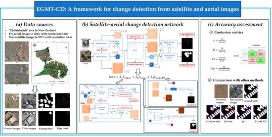
Huge difference in resolution between satellite and aerial images. Due to satellite and aircraft having different shooting heights and sensors, a satellite image’s resolution is usually lower than that of aerial images. A HR satellite’s resolution is approximately 0.5–2 m [8], while an aerial image’s resolution is usually lower than 0.5 m [9], and can even reach the centimeter level. Aligning the resolution of satellite and aerial image pairs through interpolation, convolution, or pooling is a direct solution to the problem, but it can cause the image to lose a large amount of detailed information and introduce some accumulated errors and speckle noise.

(2)

Blurred edges caused by complex terrain scenes and interference from the satellite and aerial image gap. Dense building clusters are often obstructed by shadow occlusion, similar ground objects, and intraclass differences caused by very different materials, resulting in blurred edges. Moreover, the parallax and inference from the lower resolution of satellite images than aerial images further increases the difficulties in change detection for buildings.

In order to solve the above problems in SACD tasks, we propose a novel network for satellite and aerial image change detection, named EGMT-CD, which combines multimodal transformers [10,11] with a sub-pixel module, adding auxiliary edge constraint to supervise feature representations’ alignment at multiple levels. More specifically, we design an improved spatially aligned transformer (SP-T) combined with a sub-pixel module to obtain the core feature and build up the resolution gaps between the satellite and aerial images. Then, we add an edge detection branch composing a dual branch decoders and designed fusion modules to enhance the interaction between the semantic level and the edge level. Finally, we integrate pixel difference information and edge information, supervised by both pixel- and edge-level constraints to generate the predicted changed buildings.

The contributions of this article are summarized as follows:

(1)

We propose a novel method, Edge-Guided Multimodal Transformers Change Detection (EGMT-CD) for heterogeneous SACD tasks, and design an imp SP-T to build up image resolution gaps. We also introduce a token loss to assist SP-T to obtain a scale-invariant core feature in the training process, which helps recover the LR satellite features to align with HR aerial features.

(2)

To overcome the blurred edges caused by complex terrain scenes and interference from the satellite–aerial image gap, we introduce a dual-branch decoder, adding an edge branch, fuse both semantic and edge information, and design an edge change loss to constrain the output change mask.

(3)

To test our proposed SACD method, we made a new satellite–aerial heterogeneous change detection dataset, named SACD. We also conducted sufficient experiments on the dataset and the results demonstrate the potential of our method for SACD tasks and show that it had the best performance by increasing the F1 score and IoU score compared to BiT (one of state-of-the-art change detection method) by 3.97% and 5.88%, respectively. The SACD dataset can be found at https://github.com/xiangyunfan/Satellite-Aerial-Change-Detection, accessed on 15 November 2023.

2. Related Work

2.1. Different Resolution for Change Detection

To address the issue of different resolutions in change detection, existing methods typically address this issue by reconstructing the image sample to make the homologous CD method suitable for SACD tasks. Statistics-based interpolation is the most direct and convenient method to match the differences between SACD images of different resolutions. However, the ability of image interpolation in information restoration is restricted. More specifically, image interpolation methods like bilinear and bicubic interpolation perform poorly in the face of large differences in resolution, resulting in more background noise and blurry edges, which increases the difficulty of feature alignment and generates many pseudo changes [12].

Besides using simplest interpolation methods, sub-pixel-based methods are studied most widely. Considering the superior performance of sub-pixel convolution to obtain high-resolution feature maps from low-resolution images [13,14,15], Ling et al. [16] first introduced sub-pixel convolution into CD to address the gap caused by different resolutions in heterogeneous images. Ling et al. adopted the principle of spatial correlation and designed a new land cover change pattern to obtain changes with sub-pixel convolution. Later, Wang et al. [17] proposed a Hopfield neural network with sub-pixel convolution to build the resolution gap between Landsat and MODIS images. Overall, compared to interpolation methods, the sub-pixel-based methods used to cleverly design a learnable up-sampling module can better reconstruct LR images. However, sub-pixel-based methods are largely restricted by the accuracy of the previous resolution feature map, focusing solely on shallow feature reconstruction without utilizing deep semantic information, resulting in the accumulation of redundant errors.

Furthermore, super resolution (SR) has been an independent task aimed to recover low-resolution (LR) images [12]. Li et al. [18] introduced an iterative super resolution CD method for Landsat-MODIS CD, which combines end-member estimation, spectral unmixing, and sub-pixel-based methods. Wu et al. [19] designed a back propagation network to obtain sub-pixel LCC maps from the soft-classification results of LR images [12]. However, SR is not flexible enough and may be limited by fixed zoom sizes in image recovery. Moreover, our ultimate goal is to achieve change detection. If we need to first build a SR dataset and train a separate SR model, the process will be very complex and time-consuming. Furthermore, the amount of data and corresponding model calculations in the SR will be very large [20]. Thus, it is imperative to bridge the huge resolution gaps and align the cross-resolution feature between paired images in SACD tasks.

2.2. Deep Learning for Change Detection

Deep learning has been widely applied in the field of remote sensing vision [21,22,23]. In CD tasks, deep learning methods have demonstrated their superiority and good generalization ability [24]. At present, deep learning CD tasks are mostly based on the Siamese Network [25], which has two identical branches. The parameters of the two branches choose whether to share the weight according to homologous or heterologous change detection. Previous research [26,27] used a Siamese Network as the encoder to extract features and calculate the changes by concatenating the features directly. Subsequent researchers improved the regional accuracy of change detection by designing various attention modules, including dense attention [28], spatial attention [29], spatial-temporal attention [14], and others. However, existing CD methods strived for the accuracy of regional changes through attention mechanisms, without realizing the importance of edge information.

Many remote sensing objects have their own unique and clear edge features, especially buildings [30]. However, most existing deep learning CD methods design various attention modules to improve the regional accuracy without utilizing building edge information. Ignoring edge information results in the poor performance of change detection in some cases, especially in heterogeneous SACD. In particular, dense building communities are often obstructed by shadow and interference from similar objects like buildings and roads, resulting in blurred edges interfering with the change detection [31]. In SACD, the lower resolution of the satellite image compared to the aerial one can worsen the above situation.

In building a segmentation task, utilizing edge information as prior knowledge can help CD networks pay attention to both semantic and boundary features [28,32,33]. Reference [34] designed an edge detection module and fused segmentation masks, with the loss function also incorporating edge optimization. Reference [35] used an edge refinement module, cooperating channel, and location attention module to enhance the ability of the network in CD tasks. Researchers in a previous study [7] fused and aligned satellite and aerial images in high-dimensional features through convolutional networks, and used the Hough method to obtain building edges as extra information to help the model focus more on building contours and spatial positions. However, existing methods only use edge information as prior knowledge and do not interact with deep semantic information, fully integrating edge features as a learnable part into the whole network.

3. Methods

This section contains five parts. First, we introduce the overall structure of our proposed network. The second part discusses our backbone, the feature extractor; the third part details the mechanism of SP-T module; the fourth part presents the dual-branch change decoders; and the last part describes our loss function.

3.1. Overview

Our proposed network (EGMT-CD) structure is shown in Figure 1 and can be divided into three parts: weight-unshared CNN feature extractors, spatially aligned transformer (SP-T), and dual branch decoders (including pixel decoder and edge decoder).

Given bitemporal images of satellite image and aerial image, $S\in R^{3\times H^{\prime }\times W^{\prime }}$ and A$\in R^{3\times H\times W}$, where $H^{\prime }$ and $H$ denote the input height, and $W^{\prime }$ and $W$ are the input width. The overall process of our EGMT-CD can be summarized as follows:

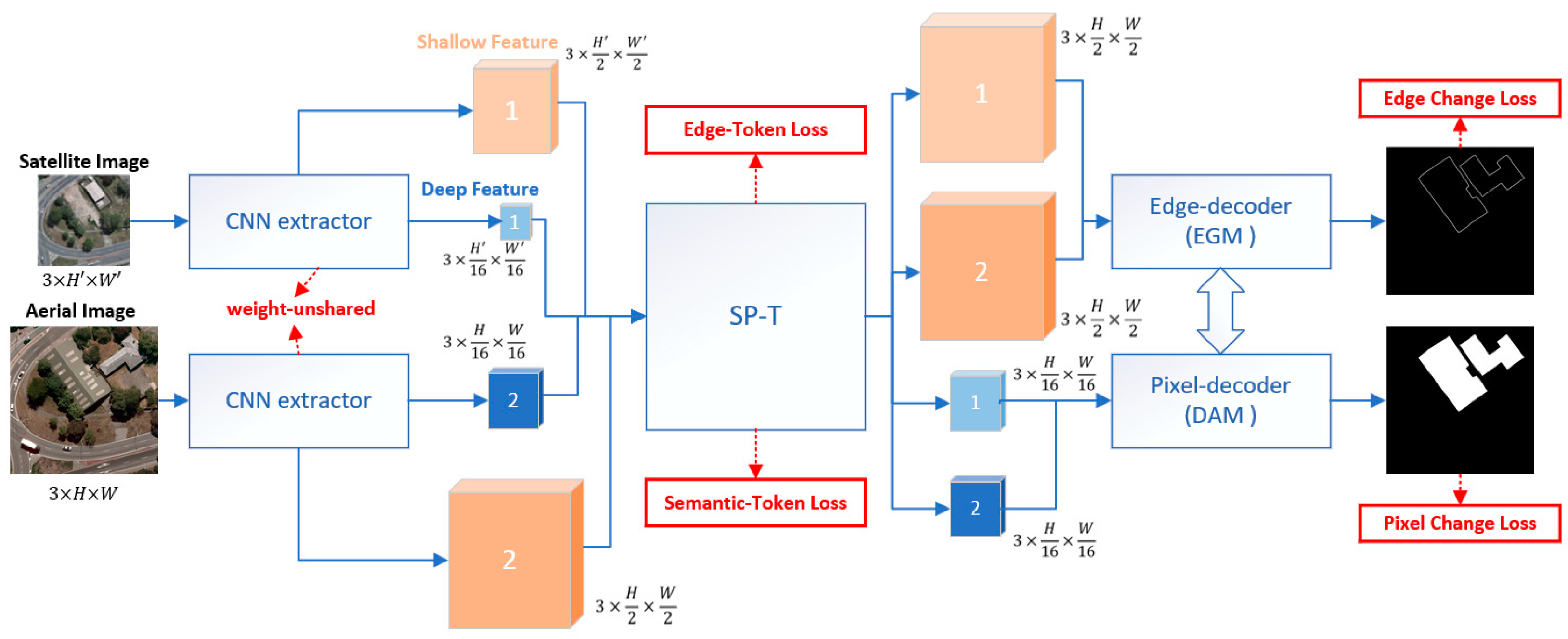
(1)

Input a pair of satellite and aerial image to the backbone based on a weight-unshared CNN Siamese Network and extract the bitemporal features, including shallow features (edge level), ${eg}^{\prime }\in R^{3\times \frac{H^{\prime }}{2}\times \frac{W^{\prime }}{2}},eg\in R^{3\times \frac{H}{2}\times \frac{W}{2}}$, and deep features (semantic level), ${se}^{\prime }\in R^{3\times \frac{H^{\prime }}{16}\times \frac{W^{\prime }}{16}},se\in R^{3\times \frac{H}{16}\times \frac{W}{16}}$.

(2)

Send the obtained features, ${eg}^{\prime }$, $eg$, ${se}^{\prime },$and $se$ into the improved spatially aligned transformer (SP-T) to recover ${eg}^{\prime }$ and ${se}^{\prime }$ to the same size with target features $eg$ and $se$. We adopted the idea of super resolution to simulate the sampling process and combined SP-T with sub-pixel convolution to achieve feature alignment. Obtain spatially aligned feature both in the edge level and semantic level, ${eg}^{\prime }\in R^{3\times \frac{H}{2}\times \frac{W}{2}}$, ${se}^{\prime }\in R^{3\times \frac{H}{16}\times \frac{W}{16}}$.

(3)

Decode and predict the change area using dual branch decoders, including an edge decoder and a pixel decoder. Input ${se}^{\prime }$ and $se$ into the pixel decoder, go through using Difference Analysis Module (DAM) and concatenate the edge decoder branch result to generate the pixel change map. Input ${eg}^{\prime }$ and $eg$ into the edge decoder, go through using Edge-Guided Module (EGM) and combine the pixel decoder branch result to obtain the edge change result.

3.2. Backbone

Classic change detection from homologous images often uses a weight-shared CNN Siamese network as backbone to simultaneously extract bitemporal features. However, the ground resolution and other features of satellite and aerial images are quite different. It was not possible to use general homogeneous change detection networks on account of the above reasons. Image interpolation methods, such as bilinear and bicubic interpolation, may be the straightforward way to solve the satellite and aerial image mismatched problem. However, image interpolation only uses a small number of surrounding pixel information and its drawbacks are obvious. It will generate a lot of noise or could confuse some information in the reconstruction map, which may lead to blurred edges of ground objects, a confused texture, and lack of detailed information, creating difficulties in the following change detection.

Thus, we adopted a weight-unshared Siamese Convolutional Neural Network (CNN) as our backbone for the purpose of extracting features from satellite and aerial images separately without interference. The structure of weight-unshared Siamese CNN as our backbone is shown in Figure 2. We modified ResNet-34 [36] to encode multiscale features. Since the two branches of Siamese Network are completely identical, we take the aerial image branch as an example here. First, we sent an aerial image to 7 × 7 convolutional layer with stride size of 2, followed by a 2 × 2 max-pooling and the input reduced to half its original size. Then, we continuously passed this through four residual blocks, obtaining features with 1/4, 1/8, 1/16, and 1/16 of the original size, and the channel was 64, 128, 256, and 512, respectively. Considering that the edge information as low-level features will disappear in the deep convolution, we concatenated the first unsampled residual block output and max-pooling output to obtain the edge feature. To obtain features of multi-scale information, the output features of all residual blocks adjusted channels of 96 channels by a 1 × 1 convolutional layer. Furthermore, they were fused together by resizing them to the same size and concatenating them into a single whole. Finally, this went through SE module to obtain the final semantic feature.

3.3. Spatially Aligned Transformer (SP-T)

The purpose of the SP-T is to achieve feature alignment both at the edge and semantic level between bitemporal features from satellite and aviation at different scales. The most convenient solution mentioned earlier is image interpolation, but the performance of change detection after direct interpolation is not satisfactory. Therefore, we used the modified SP-T in MM-Trans [20], introducing a transformer block combined with sub-pixel module and a supervised token-aligned learning strategy to resample the low resolution (LR) feature with the same size of the high resolution (HR) one. We introduced a sub-pixel module [37] to replace the interpolation part in SP-T, so that the up-sampling process integrated into the overall network as a learnable part to reconstruct more detailed information. To better achieve feature alignment, we combined multi-scale information to construct SP-T, inputting shallow edge information and deep semantic information into weight-unshared transformer encoder for future feature fusion. This can be seen in Figure 3.

(1)

Transformer

The structure of transformer is shown in Figure 4a. The transformer contains two parts: on the left is encoder and on the right is decoder. The transformer encoder is composed of two main parts: multi-head attention (MHA) and feed forward network (FFN) [10]. Layer-normalization (LN) layers were used before MHA and FFN and residual connection was also used in every step. Given a feature f, the process of transformer can be summarized as follows:

First, we turn the input feature f into token embedding with a 1 × 1 convolution, setting the token length of l = 4. Then, the encoder (left part) encodes the contextual information in token embedding as shown in Formula (1). The MHA contains h = 8 weight-unshared heads and each head used three linear layers to transform the token embedding into three tensors (query (Q), key (K), value (V)), $\in R^{\mathrm{B}\times \mathrm{h}\times \mathrm{l}\times \mathrm{d}}$, followed by self-attention as shown in Formulas (2) and (3). B is batch size and d = 64 is the dimension of Q, K, and V. Next, the output of MHA is sent into FFN, with two linear transformations with a Gaussian error linear unit (GeLU) activation [38], in order to provide nonlinear transformation and enhancement of embedding features. The output of the FFN is shown in Formula (4).

$$t=MHA(LN\left(emb\left(f\right)\right)+emb\left(f\right)$$

(1)

$$Q, K, V={linear}_Q\left(t\right),{linear}_K\left(t\right), {linear}_V\left(t\right)$$

(2)

$$Attention\left(Q, K, V\right)=Softmax\left(\frac{Q{K}^T}{\sqrt{d}}\right)V$$

(3)

$$t=FFN\left(LN\left(t\right)\right)+t$$

(4)

Finally, the decoder (right part) was used to associate the semantic global information with the input to obtain the decoding feature f’. The decoder was almost the same as the encoder, and the only difference was the source of Q, K, and V. It takes cross attention [39] to learn the correlation between f and t, which means Q is from the decoder and K and V are from the encoder.

(2)

Sub-pixel Convolution

A process of sub-pixel convolution is shown in Figure 4b. The sub-pixel module is a simple, practical, and learnable up-sampling module, cleverly rearranging low-resolution channels into high-resolution feature maps to reconstruct the resolution of the image. Variable r represents the sub-pixel scale size and the value of r is set to 3. The size of the input feature is $H\times W\times r^2$. After the sub-pixel convolution, input feature is rearranged to a high-resolution reconstructed image with the size of $rH\times r W\times 1$.

(3)

SP-T

The process of SP-T is shown in Figure 3. An improved token-aligned SP-T was employed here to enhance the feature alignment at both the edge and semantic level. First, HR feature $A_{HR}\in R^{3\times (\mathrm{H}/2)\times (\mathrm{W}/2)}$ and $B_{HR}\in {\mathrm{R}}^{3\times (H/16)\times (W/16)}$ were bicubically interpolated to a simulated LR feature $A_{HR}^{\downarrow }$ and $B_{HR}^{\downarrow }$ with the same size of $A_{LR}$ and $B_{LR}$, $A_{LR}\in {\mathrm{R}}^{3\times ({\mathrm{H}}^{\prime }/2)\times ({\mathrm{W}}^{\prime }/2)}$ and $B_{HR}\in {\mathrm{R}}^{3\times ({\mathrm{H}}^{\prime }/16)\times ({\mathrm{W}}^{\prime }/16)}$. Then, $A_{HR}$ and $B_{HR}$, and $A_{HR}^{\downarrow }$ and $B_{HR}^{\downarrow }$ were sent to the weight-unshared transformer encoders to obtain their token representations, ${A_{HR}}^{\prime }$ and ${B_{HR}}^{\prime }$, and ${A_{HR}^{\downarrow }}^{\prime }$ and ${B_{HR}^{\downarrow }}^{\prime }$. The learnable token embedding can be denoted as:

$${token}_{edge} loss={\left({A_{HR}}^{\prime }-{A_{HR}^{\downarrow }}^{\prime }\right)}^2$$

(5)

$${token}_{semantic} loss={\left({B_{HR}}^{\prime }-{B_{HR}^{\downarrow }}^{\prime }\right)}^2$$

(6)

$$tokenloss=({token}_{edge} loss+{token}_{semantic} loss)/2$$

(7)

By optimizing the token loss, the difference between low-resolution satellite image and high-resolution aerial image can be reduced. The transformer encoder of SP-T can capture similar multi-level information from raw aerial images and down-sampling simulated low-resolution images. Thus, the SP-T can capture more essential scale-invariant features for efficient alignment between low-resolution satellite images and high-resolution aerial images constrained by the token loss.

Then, we adopted the sub-pixel module to reconstruct $A_{LR}$ and $B_{LR}$ to $A_{LRs}$ and $B_{LRs}$ with the same size of $A_{HR}$ and $B_{HR}$. The sub-pixel module is a useful up-sampling method, combining individual pixels on multi-channel features into units on a single feature. The pixels on each channel are equivalent to sub-pixels on the reconstructed feature. Input $A_{LRs}$ and $B_{LRs}$ were input to the transformer encoders to obtain the transferred feature, ${A_{LR}}^{\prime }$ and ${B_{LR}}^{\prime }$.

Finally, through the transformer decoders fusing the contextual information and the transferred input, $A_{LRs}$ and $B_{LRs}$, we obtained the final reconstructed features, $A_{LR\to HR}\in R^{3\times (\mathrm{H}/2)\times (\mathrm{W}/2)}$ and $B_{LR\to HR}\in R^{3\times (\mathrm{H}/16)\times (\mathrm{W}/16)}$, which had the same size of $A_{HR}$ and $B_{HR}$.

3.4. Dual-Branch Decoders

3.4.1. Pixel Decoder

Our pixel decoder consists of two parts: one is Difference Analysis Module (DAM), which was used to enhance the dissimilarity between changed feature pairs, and the other was the usual process going from feature extraction to prediction results. The structure of the pixel decoder is shown in Figure 5.

To obtain enhanced and accurate difference information, a DAM was constructed via analyzing the correlation between feature pairs. The transformer decoder was used to initially measure the similarity between features pairs. Compared to linear difference analysis methods, the transformer decoder can capture the global information and obtain more accurate change detection results. The transformer output multiplies the difference between the feature pairs, generating the final accurate difference feature for pixel change detection predictions. In this way, the DAM can effectively enhance the difference information. The DAM can be formulated as follows:

$$F_{out}=Trans(F_1-F_2)\times |F_1-F_2|$$

(8)

Finally, we utilized a prediction head to obtain pixel change results. The semantic feature was up-sampled and concatenated with the edge feature. Then, the fused changed features were up-sampled to the same size as the original input size and went through SoftMax classifier to obtain the final pixel change map. The semantic feature fused with the edge feature can both obtain the changed buildings edges, and integrate edge information to obtain the more precise predicted change results.

3.4.2. Edge Decoder

To reduce interference from blurry edges caused by complex terrain scenes and sat-aerial image resolution gap, and alleviate the missing detection of changed buildings, we introduced an edge detect branch to guide change detection. Edge information contains both a building’s boundary shape and geographic location. Adding edge information will effectively supervise the training of buildings change detection to obtain finer prediction results, especially around the areas with dense building clusters.

The edge decoder interacted with the pixel decoder, fully fusing shallow edges and deep semantic information to achieve better change detection results, and its structure is shown in Figure 6. Although the shallow feature provides useful edge information, it also contains complicated background noise. We adopted an easy attention module, Edge Self Attention (ESA), to alleviate background noise. This module utilizes deep semantic information to help remove background noise from shallow features. The process of ESA can be summarized as follows:

$$F_{out}=Conv2D\left(sigmoid\right(upsample\left(F_{sem}\right)\times F_{edge}\left)\right)$$

(9)

where $F_{sem}$ represents the semantic feature from change decoder and $F_{edge}$ represents the edge feature after fusion. Our up-sampling used bilinear interpolation algorithm to recover semantic features back to the same size as shallow features. Sigmoid was the activation function used, and then the dot product between the attention map of semantic and edge features reduces the background noise in the edge feature map.

3.5. Loss Function

In order to effectively guide continuous optimization of the performance of model during training, it was important to construct adequate loss function and balance the weight of each part. Our loss function contained three main parts: token loss, pixel change loss, and edge change loss. Pixel change loss is the traditional one, used to supervise the predicted change results at the pixel level. Token loss helps the low resolution of a satellite image to be reconstructed and aligned with the aerial image. Edge change loss supervises the result of the edge detection and helps obtain better change boundaries. The loss function can be formulated as follows:

$$loss={\lambda }_1{L}_{pixel}+{\lambda }_2{L}_{token}+{\lambda }_3{L}_{edge}$$

(10)

where $L_{pixel}$ represents the focal loss [40], and $L_{token}$ and $L_{edge}$ both use the basic loss, mean squared error (MSE). λ₁, λ₂, and λ₃ are the weights used to balance the whole function. These weights were set to 0.7, 0.3, and 0 in the first 30 epochs. After that, these weights were changed to 0.7, 0.1, and 0.2.

Focal loss represents some progress over the binary cross-entropy loss function. Focal loss is used in the image field to alleviate data imbalance problems between the large number of background pixels and small number of objects. Its formula is expressed as follows:

$$L_{pixel}\left\{\begin{array}{c}-\alpha {\left(1-p\right)}^{\gamma }\log \left(p\right), if y=1\\ -\left(1-\alpha \right)p^{\gamma }\log \left(p\right), if y=0\end{array}\right.$$

(11)

where p denotes the predicted result and y represents the change label. We set the value of $\alpha ,$ $\gamma$ to control the weights of positive and negative samples and calculate the overall loss. The parameters $\alpha ,$ $\gamma$ represent the focusing parameter, and ${\left(1-p\right)}^{\gamma }$ denotes a modulating factor. The modulation factor can reduce the weight of easily separable samples, helping the network to pay more attention to the hard samples to separate during the training process. Specifically, parameters of α = 0.3 and γ = 2.0 were used.

MSE loss measures the accuracy of the model by calculating the average square difference between the predicted value and the true value. It can be formula as follows:

$$L_{token}, L_{edge}=\frac{1}{N}{\sum }_{n=1}^N{(X_N-Y_N)}^2$$

(12)

where X denotes the change labeled, Y denotes the predicted results, and N represents the total number of labels.

4. Experiments

In this section, we talk about the dataset, experimental details, evaluation metrics, and comparison methods used in the experiments.

4.1. Dataset

To verify the effectiveness and superiority of the method proposed in this paper, we created a satellite and aerial image heterogenous change detection dataset (SACD), with the aim of providing a standard satellite–aerial heterogenous dataset to fairly compare the performance of various change detection algorithms. The SACD dataset covers Christchurch, New Zealand, and its surrounding areas, with an area of approximately 20.5 square kilometers. The region experienced a 6.3 magnitude earthquake in February 2011 and underwent reconstruction in the following years. The dataset contains two image scenes, which are composed of aerial images from 2012 and satellite imagery from 2017. SACD focuses on urban areas and focuses on changes in urban buildings. In 2012, the image included 12,796 buildings (in 2017, the same area included 16,897 buildings). The overview of our SACD dataset is depicted in Figure 7.

The production process of the SACD dataset included image download, manual registration, resampling, sample labeling, and slicing. The aerial image was from the WHU public data set [41], and for the satellite imagery we selected the 18-level image of Google Earth in Bigemap through the corresponding longitude and latitude information. The SACD dataset covers areas with latitude and longitude ranging from (172.506899°, −43.537200°) to (172.587176°, −43.565168°). The size of the satellite imagery was 11 K × 6 K pixels. The ground resolution of the satellite imagery and aerial image was 0.6 m and 0.2 m, respectively. The image was manually selected with ENVI control points and registered using the polynomial method, consisting of 336 control points with RMS Error = 2.0389. After registration, we manually generated ground truth labels pixel by pixel by comparing two images. Afterwards, this aerial image was cropped to a size of 384 × 384 for experimentation, while Google Earth Image was correspondingly cropped to a size of 128 × 128. A total of 3400 samples were generated and divided into training, validation, and testing sets at a 7:1:2 ratio. In order to achieve boundary constraints and supervision on SACD, we adopted the Canny edge detection algorithm that is not easily affected by noise to obtain corresponding changing edge labels. The Canny algorithm thresholds were set to 70 and 130. Some examples of our SACD dataset are shown in Figure 8, including aerial and satellite images in the pre- and post-earthquake phases, pixel level labels, and boundary labels.

4.2. Experimental Details

We implemented our model in PyTorch and trained it using two NVIDIA RTX 3090 GPUs (24 G memory). To ensure the fairness of our experiment, we adopted identical data preparation and augmentation practices and ensured that each model could realize its potential while considering similar parameters. First, we took several data augmentation steps to enhance our dataset samples, which could increase the robustness of our model. Data augmentation contains random transposition, flipping, rescaling (0.9–1.1), Gaussian blur, and HSV color vibrance. All the data augmentation methods mentioned above have a probability of 0.3. During the training process, we chose the optimizer as AdamW with parameter β values of (0.9, 0.999) and the weight attenuation was 0.01. The networks initiated randomly and adopted a linear learning strategy with an initial value of 0.002 that decreased each epoch. The batch size depended on each model and the number of epochs was set to 100. As for our loss, we discussed this in Section 3.5 and we used both focal loss and MSE. We chose focal loss to overcome the imbalance problem between the large area of the background and the small area of the object. Moreover, we designed an edge change loss to assist the original loss, using the edge constraint to obtain more precise and fine change results. Since adding auxiliary losses may interfere with model training, balancing the entire loss function was crucial.

4.3. Evaluation Metrics

To evaluate the results, we used universal quantitative evaluation indicators to evaluate the effectiveness of the model in this study: precision (P), recall (R), F1 score, and intersection over union (IoU). The indicators’ formulas are as follows:

$$P=\frac{TP}{TP+FP}$$

(13)

$$R=\frac{TP}{TP+FN}$$

(14)

$$F1=\frac{2\times P\times R}{P+R}$$

(15)

$$IoU=\frac{TP}{TP+FP+FN}$$

(16)

Predicting results on test datasets compared with labels typically generates four different types of pixels, equally forming a confusion matrix with TP, FP, FN, and FP. TP denotes the number of predictions that are true and positive; FP denotes the number of predictions that are false and positive; FN denotes the number of predictions that are false and negative; and FP denotes the number of predictions that are false and positive. Precision (P) calculates the proportion of TPs among all the predicted change pixels and reflects the model’s ability to predict the correct object. Recall (R) calculates the proportion of TPs among the real change pixels and reflects the model’s ability to find completely correct objects. The F1 score is a comprehensive indicator that takes into account both P and R. IoU represents the ratio of the intersection and union of the predicted and actual changing pixels, measuring the similarity between the prediction and label. Each indicator may pay attention to a different aspect of performance through various methods; therefore, we need a comprehensive evaluation.

4.4. Comparison Methods

To verify the effectiveness of the proposed method, we conducted comparative experiments with several good performing methods. In order to enable the homologous change detection algorithm to process heterogeneous data from aviation and satellite sources, we use bicubic interpolation to up-sample the satellite images to the same size as aerial images for subsequent change detection. We selected classic CD networks and state-of-the-art CD networks for comparisons. FC-EF, FC-Siam-Conc, and FC-Siam-Diff are classic fully convolution-based CD networks. STANet and SNUNet are attention-based methods. BITNet is the state of-the-art building CD network introducing a transformer. The networks’ descriptions are as follows:

(1)

FC-EF [14,42]: The network adopts the early fusion of features. It is similar to the U-Net structure, and it directly fuses pre and post images in the channel dimension and sends these into the network.

(2)

FC-Siam-conc [14,42]: The network combines an FC-EF structure with a Siamese Network, which adopts an identical encoder with shared weights and concatenates the feature difference to predict change results.

(3)

FC-Siam-diff [14,42]: The network is improved using FC-Siam-conc, which changes the fusion strategy of hierarchical feature maps from concatenation to the absolute value of the difference.

(4)

STANet [16]: This is a method introduced for the spatial-temporal attention mechanism to adjust weights in the space and time dimensions between two paired images to obtain the location and better distinguish changes.

(5)

SNUNet-CD [43]: This is a channel attention-based method inspired by the structure of the NestedUNet [44]. The network introduces dense connections and a large number of skip connections to deeply mine multiscale features. Furthermore, the channel attention module (ECAM) is used to assign appropriate weights to semantic features at different levels to obtain better overall change information

(6)

BIT [45]: This is a method embedded with a transformer module in a Siamese network. The network adopts an improved ResNet-18 as its backbone [36], introducing a bitemporal image transformer to map pre and post temporal images to global contextual information, aiming to capture the core difference from the high-level semantic token.

5. Results

To verify the effectiveness of our proposed method, we compared classic and superior change detection methods with our proposed model and conducted a considerable number of ablation study experiments.

5.1. Comparisons of the SACD Dataset

To test the effectiveness and progressiveness of our proposed method, we conducted many experiments and compared several superior existing change detection methods with our network, EGMT-CD. Notably, all the networks were performed under the same data augmentations and experimental settings to obtain fair and comparative results. The results are shown in

Table 1. Quantitative performance comparison on the SACD dataset.

Network	Precision	Recall	F1 Score	IoU
FC-EF	69.97	71.70	70.82	54.83
FC-Siam-Conc	70.59	74.02	72.26	56.57
FC-Siam-Diff	73.35	71.58	72.45	56.81
STANet	85.05	69.79	76.67	62.16
SNUNet-CD	76.73	82.78	79.64	66.17
BiT	80.48	83.06	81.75	69.13
EGMT-CD(ours)	84.08	87.43	85.72	75.01

and Figure 9.

Table 1 shows the results of the quantitative evaluation of the SACD dataset. It is obvious that our method had significantly improved results compared to the other methods with satellite–aerial heterogeneous datasets, which suggests that our method is effective for satellite and aerial image change detection. The EGMT-CD model (our model) achieved the best results on most metrics, with an F1 score of 85.72% and an IoU score of 75.01%. The F1 score and IoU score increased by 3.97% and 5.88%, respectively, compared to the BiT method. Precision values also basically reached the best level, which was only 0.97% lower than the highest performing model. The STANet model achieved the highest precision values of 85.05%, but it was not balanced, with a recall score of only 69.79%, which was far lower than the EGMT-CD model (our model). This means that the STANet model failed to detect small change areas and was insensitive to changes in object edges. Above all, the EGMT-CD model (our model) performed the best overall, especially given its recall value of 87.43%, which means the model rarely missed small, insignificant, and confusing areas of change. The EGMT-CD model (our model) also had a significantly better performance than the other networks in terms of the F1 score and IoU, which directly reflects its superior performance in our experiments.

We visualized all CD network test results on our SACD dataset. Figure 9 shows the prediction performance of each network model in various scenarios. Each row represents a set of test data and there are six rows in total. The first two columns represent the pre-temporal aerial image and post-temporal satellite image. The third column represents the changing labels, and after this represents the predicted results of each network. We use different colors in our drawings to represent different test results White represents true positive pixels with a correct change (TP). Black represents true negative pixels with an incorrect non-change (TN). Blue indicates false negative pixels meaning a false change (FP). Red indicates false negative pixels meaning a missed change (FN).

From the results shown in Figure 9, the following points can be seen:

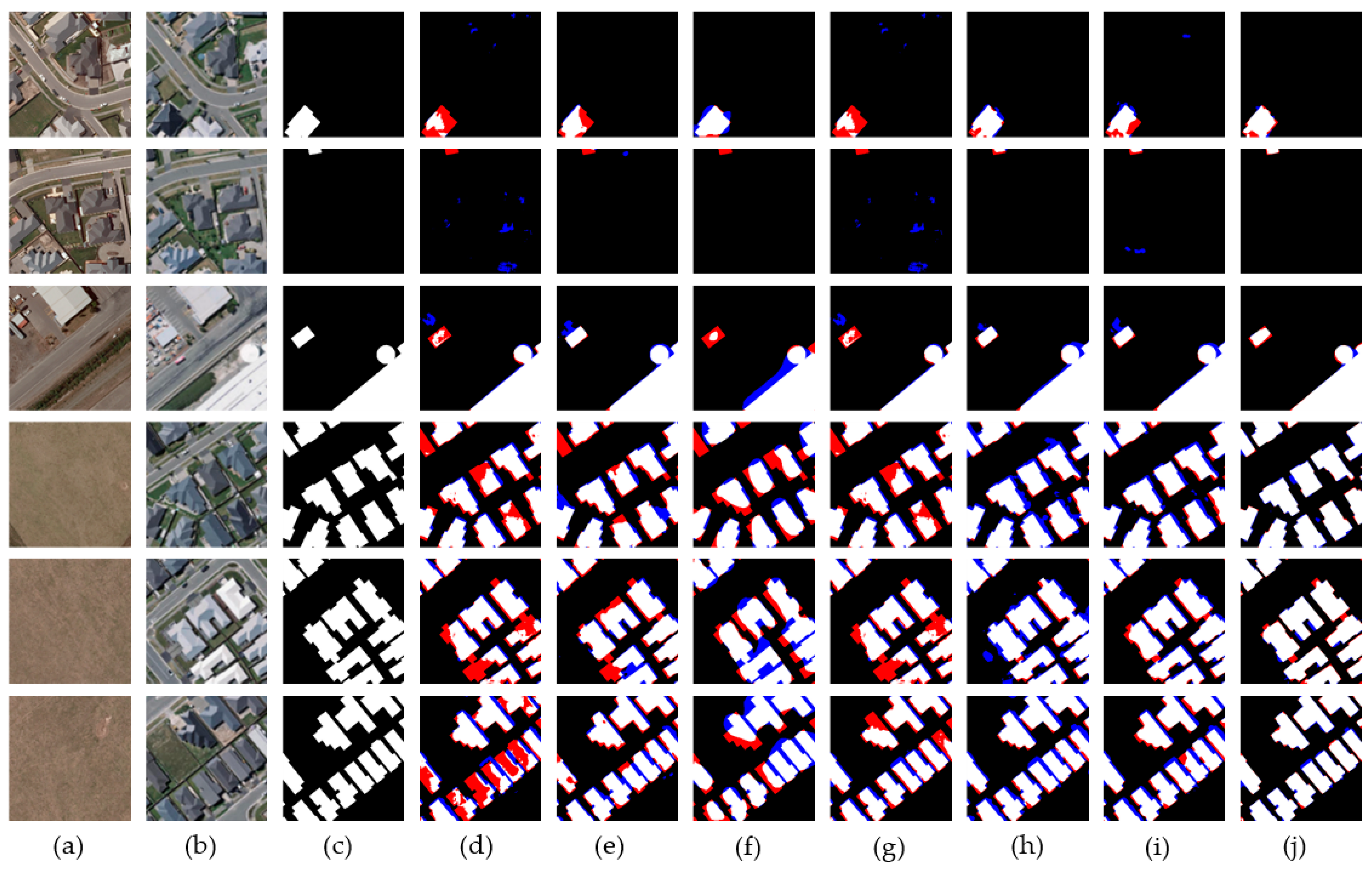
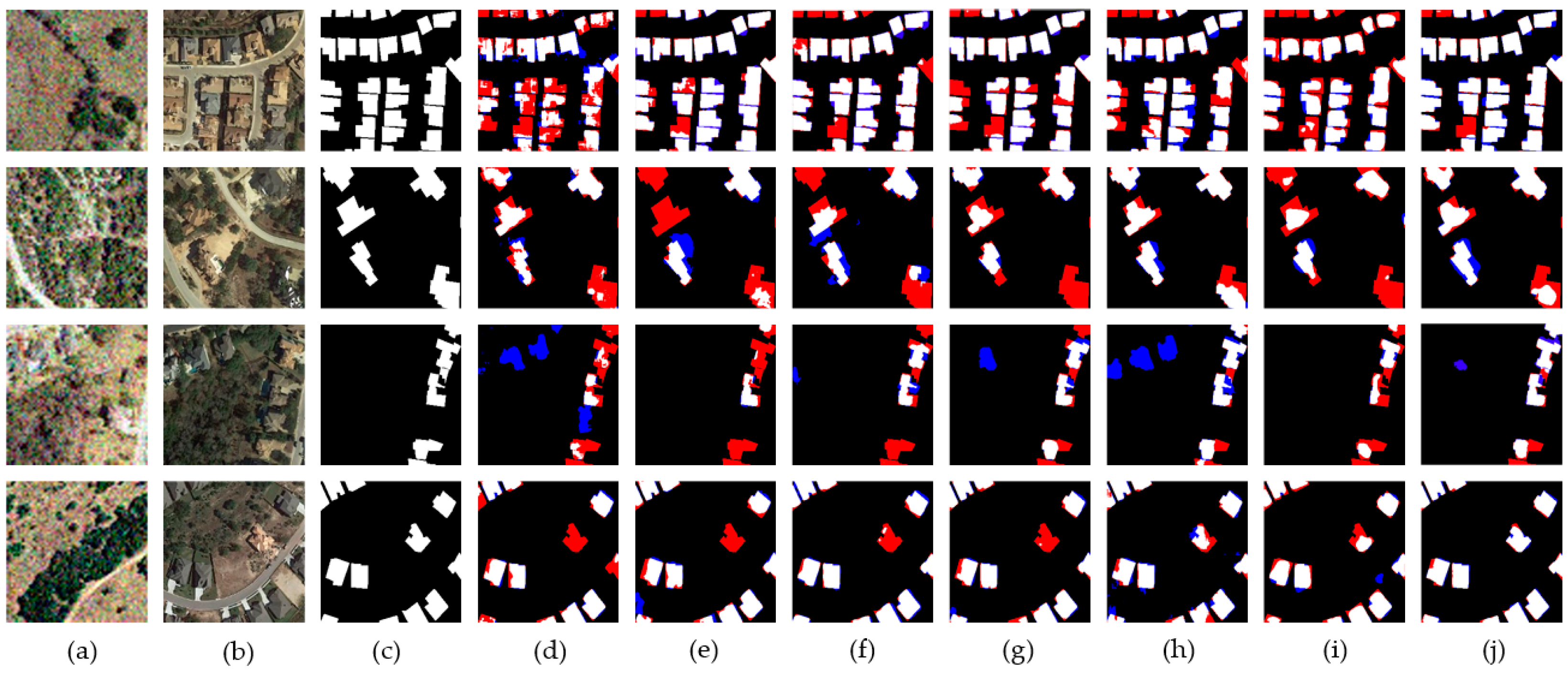
(1)

It is very difficult to detect small changes in complex building clusters in pre- and post-event image pairs. The resolution gap between satellite and aerial images further aggravates this difficulty, making small buildings blurrier and narrowing feature dissimilarity from the background and other objects. As shown in Figure 9, we can see that EGMT-CD effectively captured small building changes, and the phenomenon of missed detections (the red marked area) was significantly improved. In contrast, other CD networks failed to correctly identify changing areas on account of the resolution gap.

(2)

It is hard to identify each changed building shape in densely connected building areas. The resolution gap and parallax from satellite and ariel image pairs also worsens the situation, as the building object edge is much harder to determine and match. As shown in Figure 9, the EGMT-CD model could reduce the boundary noise of the changing region and obtained finer region boundary descriptions than the other CD networks (the blue marked area).

5.2. Ablation Study

5.2.1. Ablation Study of Each Component in EGMT-CD

To verify the strength of each module proposed in this paper, we conducted ablation experiments to test the performance of adding the spatially aligned transformer (SP-T) module, edge detection branch (EDB), and difference analysis module (DAM) on the SACD dataset. The ablation results are shown in

Table 2. Quantitative performance comparison on ablation study.

Baseline	DAM	SP-T	EDB	Precision	Recall	F1 Score	IoU
√				76.47	74.62	75.53	60.69
√	√			78.28	77.90	78.09	64.05
√	√	√		82.05	84.36	83.19	71.22
√	√		√	83.84	79.06	81.37	68.61
√	√	√	√	84.08	87.43	85.72	75.01

We set up five sets of ablation experiments. As shown in Table 2, the first row is our baseline model and it used a weight-unshared Resnet34 Siamese network as the backbone, and then directly concatenated the extracted pre- and post-temporal features and then up-sampled to obtain the final changing maps. The second row shows the evaluation of the performance improvement brought by using the DAM. The third to fifth rows explore the SP-T and EDB to examine which module contributed more to the improvement of sat-aerial image multimodal change detection, and whether the effect of the combination of the two modules was much better.

Table 2 suggests that all the networks using the DAM had an obviously improved change detection performance compared to the network without the DAM. From the comparison between the first and second rows, it is most obvious that all evaluation indicators improved, especially the F1 score and the IoU score, which increased by 2.56% and 3.36%, respectively, compared to the baseline method, which means the DAM can effectively enhance the differences between change features through the self-attention mechanism. Comparing the second row with the third and fourth rows, adding either the SP-T or EDB greatly improved the evaluation metrics. The difference was that the SP-T module focuses more on the improvement of the recall score, which achieved the second highest score of 84.36%, while the EDM contributed a lot to the precision score, also reaching the second highest score of 83.84%. From the perspective of the F1 and IoU scores, the addition of SP-T was more beneficial than the EDM, with F1 and IoU scores that were 1.82% and 2.61% higher, respectively. It is reasonable to state that the SP-T solved the main problem of the resolution gap between the satellite and aerial images, while the EDB optimized the edge detection and added an edge constraint to obtain a fine boundary of change detection. The addition of all modules in the last row achieved the best performance of the whole evaluation metrics (F1 and IoU scores of 85.72% and 75.01%), further demonstrating the effectiveness and compatibility of our proposed modules.

Moreover, our conclusion can be intuitively seen from Figure 10. After introducing the DAM into the structure of the baseline in the second row, the predicted change area had fewer red and blue marked areas, representing its relatively high precision and recall score. After adding the SP-T to the model in the third row, the red marked missed detection area was substantially reduced due to the alignment of the satellite–aerial resolution gap. In contrast, the addition of the EDM obtained a finer boundary of the changing buildings corresponding to very few blue marked areas in the fourth row. As a matter of fact, our method, EGMT-CD, incorporated with all three modules performed the best, with rare omissions and clear building outlines in the last row, overcoming the resolution differences and interference from complex scenes.

5.2.2. Ablation Study of Loss Function Parameters

As discussed in Section 3.5, our loss function contained three parts, including pixel change loss, token loss, and edge change loss. We used parameters λ₁, λ₂, and λ₃ to balance the loss. Due to the significant impact of parameter values on training results, we conducted an experiment to analyze the relationship between the performance of the EGMT-CD model and the parameter values in order to obtain the best results.

First, we need to address the main issue of the resolution gap between satellite and aerial images. We set the edge change loss parameter λ₃ to 0 at the beginning because the model will find it difficult to converge if all parts of the loss function were simultaneously optimized. The value of pixel change loss parameter λ₁ equaled 1 − λ₂. Thus, we adjusted the token loss parameter λ₂ to explore the best performance of our model training as shown in Figure 11. It was clear that λ₂ = 0.3 (λ₁ = 0.7) was the most suitable value for our model.

Next, we further added the auxiliary loss of edge changes to obtain more refined change results. After multiple experiments, it was suitable to introduce the edge change loss after a stable token loss of 30 epochs. Then, we set the value of parameter λ₂ to 0.1 to maintain a small adjustment space. The value of pixel change loss parameter λ₁ equaled 0.9 − λ₃. Thus, we then adjusted the edge loss parameter λ₃ to establish the suitable weight value for our model. As shown in Figure 12, it was easy to find out that the model performed best when the parameter value of λ₃ = 0.2 (λ₁ = 0.7).

6. Discussion

In this section, we want to explore the generalization ability and efficiency of various models for SACD tasks. Thus, we conducted another experiment on the publicly available CD dataset, LEVIR-CD [16], down-sampling to simulate the SACD task. The LEVIR-CD dataset contains 637 images of 1024 ×1024 with a resolution of 0.5 m. We cut the dataset into 256 × 256 and divided it into training, validation, and testing sets at a 7:1:2 ratio. In order to simulate the SACD task as realistically as possible, we down-sampled the pre-temporal images using nearest neighbor and linear interpolation, and added Gaussian noise with a mean of 0 and a standard deviation of 1, as well as salt and pepper noise with a probability of 0.01. Although this cannot fully simulate the real situation due to image registration and the more complex information of heterogeneous images, it could verify the robustness of the model to a certain extent. We implemented all comparison methods without any data augmentation, and the experimental results are shown in

Table 3. Quantitative comprehensive performance comparison on the LEVIR-CD dataset.

Network	F1 (%)	IoU (%)	Params (M)	FLOPs (G)
FC-EF	75.71	60.92	1.35	3.55
FC-Siam-Conc	79.85	66.46	1.54	5.29
FC-Siam-Diff	77.42	63.16	1.35	4.68
STANet	82.14	69.69	16.93	40.45
SNUNet-CD	83.21	71.25	12.03	54.82
BiT	83.08	71.06	11.48	26.29
EGMT-CD (ours)	86.36	75.99	36.27	37.52

. Here, we have introduced two new indicators for evaluation, Params and FLOPs. The Params is the size of the model’s parameters, measured in M (${10}^{-6}$), which reflects the spatial complexity. The FLOPs is the “floating-point operations per second”, measured in G (${10}^{-9}$), which represents the time complexity and computational complexity.

From Table 3, we can see that the three methods based on FC had the smallest Params and FLOPs values, but their performance in SACD was also below the others. The STANet, SNUNet CD, and BiT methods achieved an almost better performance based on the F1 and IOU values due to their incorporation of various attention mechanism designed into the basic network architecture. While there was not much difference in Params among these three methods (16.93 M, 12.03 M, 11.48 M), it can be seen that the transformer-based method BiT (26.26 G) had certain advantages over the other two CNN-based methods (40.45 G, 54.85 G) in terms of computational efficiency, FLOPs. Our proposed method EGMT-CD was also based on the transformer and achieved the best results in all accuracy indicators, with an F1 score of 86.36% and an IoU score of 75.99%, at the cost of relatively large parameters and computational costs. Our model still maintained an advantage in computational efficiency compared to the CNN-based method, with FLOPs of 37.52 G, but the Params value of 36.27 M was much higher on account of integrating the super-resolution module and edge detection branch into the change detection network for SACD tasks. From Figure 13, we can directly see that our method, EGMT-CD, had an obvious improvement in accuracy for SACD tasks in visualization, with the red and blue parts in the figure being significantly rarer than other methods.

In summary, we believe that future research can be optimized in two directions. One is the lightweighting of the model, which includes introducing lightweight modules and considering the reuse of similar functional modules. The other is about image registration, which has a significant impact on the performance of change detection, especially for heterogeneous images. We have gained this vision after simulating SACD tasks using public CD datasets.

7. Conclusions

In this paper, we propose a novel satellite–aerial change detection method based on Edge-Guided Multimodal Transformers (EGMT-CD), which obviously improved the performance of satellite–aerial heterogeneous change detection. In order to cope with various ground resolution and blurred edge boundaries caused by multiple factors, including occlusion and interference from the satellite–aerial image gap, the EGMT-CD adopts a weight-unshared Siamese CNN backbone to independently extract the bitemporal features. Moreover, we designed an improved SP-T combined with sub-pixel convolution to obtain scale-invariant feature representations and bridge the gap in resolution between satellite and aerial images supervised by a token loss. Furthermore, we introduced an edge branch and constraint change map with auxiliary edge loss to improve the building edge detection performance in order to be adequate for SACD tasks. The ablation study on EGMT-CD proved the effectiveness of the SP-T and the edge branch. We also created a new dataset for satellite–aerial change detection tasks. The comparative experiments on the SACD dataset many superior CD methods have demonstrated the potential of the EGMT-CD in the field of SACD.

References

- Jérôme, T. Change Detection. In Springer Handbook of Geographic Information; Springer: Berlin/Heidelberg, Germany, 2022; pp. 151–159. [Google Scholar]
- Hu, J.; Zhang, Y. Seasonal Change of Land-Use/Land-Cover (Lulc) Detection Using Modis Data in Rapid Urbanization Regions: A Case Study of the Pearl River Delta Region (China). IEEE J. Sel. Top. Appl. Earth Obs. Remote Sens. 2013, 6, 1913–1920. [Google Scholar] [CrossRef]
- Jensen, J.R.; Im, J. Remote Sensing Change Detection in Urban Environments. In Geo-Spatial Technologies in Urban Environments; Springer: Berlin/Heidelberg, Germany, 2007; pp. 7–31. [Google Scholar]
- Zhang, J.-F.; Xie, L.-L.; Tao, X.-X. Change Detection of Earthquake-Damaged Buildings on Remote Sensing Image and Its Application in Seismic Disaster Assessment. In Proceedings of the IGARSS 2003, 2003 IEEE International Geoscience and Remote Sensing Symposium, Proceedings (IEEE Cat. No. 03CH37477), Toulouse, France, 21–25 July 2003. [Google Scholar]
- Bitelli, G.; Camassi, R.; Gusella, L.; Mognol, A. Image Change Detection on Urban Area: The Earthquake Case. In Proceedings of the Xth ISPRS Congress, Istanbul, Turkey, 12–23 July 2004. [Google Scholar]
- Zhan, T.; Gong, M.; Jiang, X.; Li, S. Log-based transformation feature learning for change detection in heterogeneous images. IEEE Geosci. Remote Sens. Lett. 2018, 15, 1352–1356. [Google Scholar] [CrossRef]
- Shao, R.; Du, C.; Chen, H.; Li, J. SUNet: Change detection for heterogeneous remote sensing images from satellite and UAV using a dual-channel fully convolution network. Remote Sens. 2021, 13, 3750. [Google Scholar] [CrossRef]
- Lu, D.; Mausel, P.; Brondizio, E.; Moran, E. Change detection techniques. Int. J. Remote Sens. 2004, 25, 2365–2401. [Google Scholar] [CrossRef]
- Zongjian, L. UAV for mapping—Low altitude photogrammetric survey. Int. Arch. Photogram. Remote Sens. Beijing China 2008, 37, 1183–1186. [Google Scholar]
- Vaswani, A.; Shazeer, N.; Parmar, N.; Uszkoreit, J.; Jones, L.; Gomez, A.N.; Kaiser, L.; Polosukhin, I. Attention is all you need. arXiv 2017, arXiv:1706.03762. [Google Scholar]
- Bazi, Y.; Bashmal, L.; Rahhal, M.M.A.; Dayil, R.A.; Ajlan, N.A. Vision transformers for remote sensing image classification. Remote Sens. 2021, 13, 516. [Google Scholar] [CrossRef]
- Liu, M.; Shi, Q.; Marinoni, A.; He, D.; Liu, X.; Zhang, L. Super-resolution-based change detection network with stacked attention module for images with different resolutions. IEEE Trans. Geosci. Remote Sens. 2021, 60, 1–18. [Google Scholar] [CrossRef]
- Papadomanolaki, M.; Verma, S.; Vakalopoulou, M.; Gupta, S.; Karantzalos, K. Detecting urban changes with recurrent neural networks from multitemporal Sentinel-2 data. In Proceedings of the IGARSS 2019-2019 IEEE International Geoscience and Remote Sensing Symposium, Yokohama, Japan, 28 July–2 August 2019; pp. 214–217. [Google Scholar]
- Daudt, R.C.; Le Saux, B.; Boulch, A. Fully convolutional Siamese networks for change detection. In Proceedings of the 2018 25th IEEE International Conference on Image Processing (ICIP 2018), Athens, Greece, 7–10 October 2018; pp. 4063–4067. [Google Scholar]
- Daudt, R.C.; Le Saux, B.; Boulch, A.; Gousseau, Y. Urban change detection for multispectral earth observation using convolutional neural networks. In Proceedings of the IGARSS 2018-2018 IEEE International Geoscience and Remote Sensing Symposium, Valencia, Spain, 22–27 July 2018; pp. 2115–2118. [Google Scholar]
- Chen, H.; Shi, Z. A spatial-temporal attention-based method and a new dataset for remote sensing image change detection. Remote Sens. 2020, 12, 1662. [Google Scholar] [CrossRef]
- Wang, Q.; Shi, W.; Atkinson, P.M.; Li, Z. Land cover change detection at subpixel resolution with a hopfield neural network. IEEE J. Sel.Topics Appl. Earth Observ. Remote Sens. 2015, 8, 1339–1352. [Google Scholar] [CrossRef]
- Li, X.; Ling, F.; Foody, G.M.; Du, Y. A super resolution land-cover change detection method using remotely sensed images with different spatial resolutions. IEEE Trans. Geosci. Remote Sens. 2016, 54, 3822–3841. [Google Scholar] [CrossRef]
- Wu, K.; Du, Q.; Wang, Y.; Yang, Y. Supervised sub-pixel mapping for change detection from remotely sensed images with different resolutions. Remote Sens. 2017, 9, 284. [Google Scholar] [CrossRef]
- Liu, M.; Shi, Q.; Li, J.; Chai, Z. Learning token-aligned representations with multimodel transformers for different-resolution change detection. IEEE Trans. Geosci. Remote Sens. 2022, 60, 1–13. [Google Scholar] [CrossRef]
- Lin, S.; Zhang, M.; Cheng, X.; Shi, L.; Gamba, P.; Wang, H. Dynamic Low-Rank and Sparse Priors Constrained Deep Autoencoders for Hyperspectral Anomaly Detection. IEEE Trans. Instrum. Meas. 2023, 73, 2500518. [Google Scholar] [CrossRef]
- Lin, S.; Zhang, M.; Cheng, X.; Zhou, K.; Zhao, S.; Wang, H. Hyperspectral anomaly detection via sparse representation and collaborative representation. IEEE J. Sel. Top. Appl. Earth Obs. Remote Sens. 2022, 16, 946–961. [Google Scholar] [CrossRef]
- Cheng, X.; Zhang, M.; Lin, S.; Li, Y.; Wang, H. Deep Self-Representation Learning Framework for Hyperspectral Anomaly Detection. IEEE Trans. Instrum. Meas. 2023, 73, 5002016. [Google Scholar] [CrossRef]
- Bai, T.; Wang, L.; Yin, D.; Sun, K.; Chen, Y.; Li, W. Deep learning for change detection in remote sensing: A review. Geo-Spat. Inf. Sci. 2023, 26, 262–288. [Google Scholar] [CrossRef]
- Bromley, J.; Guyon, I.; Lecun, Y.; Sackinger, E.; Shah, R. Signature verification using a “siamese” time delay neural network. Int. J. Pattern Recognit. Artif. Intell. 1993, 7, 669–688. [Google Scholar] [CrossRef]
- MArabi, E.A.; Karoui, M.S.; Djerriri, K. Optical remote sensing change detection through deep siamese network. In Proceedings of the IGARSS 2018–2018 IEEE International Geoscience and Remote Sensing Symposium, Valencia, Spain, 22–27 July 2018; pp. 5041–5044. [Google Scholar]
- Zhang, M.; Xu, G.; Chen, K.; Yan, M.; Sun, X. Triplet-based semantic relation learning for aerial remote sensing image change detection. IEEE Geosci. Remote Sens. Lett. 2018, 16, 266–270. [Google Scholar] [CrossRef]
- Zheng, H.; Gong, M.; Liu, T.; Jiang, F.; Zhan, T.; Lu, D.; Zhang, M. HFA-Net: High frequency attention siamese network for building change detection in VHR remote sensing images. Pattern Recogn. 2022, 129, 108717. [Google Scholar] [CrossRef]
- Song, K.; Jiang, J. AGCDetNet: An Attention-Guided Network for Building Change Detection in High-Resolution Remote Sensing Images. IEEE J. Sel. Top. Appl. Earth Obs. Remote Sens. 2021, 14, 4816–4831. [Google Scholar] [CrossRef]
- Wei, Y.; Zhao, Z.; Song, J. Urban Building Extraction from High-Resolution Satellite Panchromatic Image Using Clustering and Edge Detection. In Proceedings of the IGARSS 2004. 2004 IEEE International Geoscience and Remote Sensing Symposium, Anchorage, AK, USA, 20–24 September 2004. [Google Scholar]
- Chen, Z.; Zhou, Y.; Wang, B.; Xu, X.; He, N.; Jin, S.; Jin, S. EGDE-Net: A building change detection method for high-resolution remote sensing imagery based on edge guidance and differential enhancement. ISPRS J. Photogramm. Remote Sens. 2022, 191, 203–222. [Google Scholar] [CrossRef]
- Zheng, Z.; Wan, Y.; Zhang, Y.; Xiang, S.; Peng, D.; Zhang, B. CLNet: Cross-layer convolutional neural network for change detection in optical remote sensing imagery. ISPRS J. Photogram. Remote Sens. 2021, 175, 247–267. [Google Scholar] [CrossRef]
- Zhou, Y.; Chen, Z.; Wang, B.; Li, S.; Liu, H.; Xu, D.; Ma, C. BOMSC-Net: Boundary Optimization and Multi-Scale Context Awareness Based Building Extraction from High-Resolution Remote Sensing Imagery. IEEE Trans. Geosci. Remote Sens. 2022, 60, 1–17. [Google Scholar] [CrossRef]
- Jung, H.; Choi, H.-S.; Kang, M. Boundary Enhancement Semantic Segmentation for Building Extraction from Remote Sensed Image. IEEE Trans. Geosci. Remote Sens. 2021, 60, 1–12. [Google Scholar] [CrossRef]
- Zhang, J.; Shao, Z.; Ding, Q.; Huang, X.; Wang, Y.; Zhou, X.; Li, D. AERNet: An attention-guided edge refinement network and a dataset for remote sensing building change detection. IEEE Trans. Geosci. Remote Sens. 2023, 61, 1–16. [Google Scholar] [CrossRef]
- He, K.; Zhang, X.; Ren, S.; Sun, J. Deep residual learning for image recognition. In Proceedings of the 2016 IEEE Conference on Computer Vision and Pattern Recognition, CVPR 2016, Las Vegas, NV, USA, 27–30 June 2016; pp. 770–778. [Google Scholar]
- Shi, W.; Caballero, J.; Huszár, F.; Totz, J.; Aitken, A.P.; Bishop, R.; Rueckert, D.; Wang, Z. Real-time single image and video super-resolution using an efficient sub-pixel convolutional neural network. In Proceedings of the 2016 IEEE Conference on Computer Vision and Pattern Recognition (CVPR), Las Vegas, NV, USA, 27–30 June 2016; pp. 1874–1883. [Google Scholar]
- Hendrycks, D.; Gimpel, K. Bridging nonlinearities and stochastic regularizers with Gaussian error linear units. arXiv 2016, arXiv:1606.08415. [Google Scholar]
- Dosovitskiy, A.; Beyer, L.; Kolesnikov, A.; Weissenborn, D.; Zhai, X.; Unterthiner, T.; Dehghani, M.; Minderer, M.; Heigold, G.; Gelly, S.; et al. An image is worth 16 × 16 words: Transformers for image recognition at scale. arXiv 2020, arXiv:2010.11929. [Google Scholar]
- Lin, T.-Y.; Goyal, P.; Girshick, R.; He, K.; Doll’ar, P. Focal loss for dense object detection. In Proceedings of the IEEE International Conference on Computer Vision, Venice, Italy, 22–29 October 2017; pp. 2980–2988. [Google Scholar]
- Ji, S.; Wei, S.; Lu, M. Fully Convolutional Networks for Multisource Building Extraction from an Open Aerial and Satellite Imagery Data Set. IEEE Trans. Geosci. Remote Sens. 2018, 57, 574–586. [Google Scholar] [CrossRef]
- Ronneberger, O.; Fischer, P.; Brox, T. U-net: Convolutional networks for biomedical image segmentation. In Proceedings of the International Conference on Medical Image Computing and Computer-Assisted Intervention, Munich, Germany, 5–9 October 2015; Springer: Berlin/Heidelberg, Germany, 2015; pp. 234–241. [Google Scholar]
- Fang, S.; Li, K.; Shao, J.; Li, Z. SNUNet-CD: A Densely Connected Siamese Network for Change Detection of VHR Images. IEEE Geosci. Remote Sens. Lett. 2021, 19, 1–5. [Google Scholar] [CrossRef]
- Zhou, Z.; Rahman Siddiquee, M.M.; Tajbakhsh, N.; Liang, J. Unet++: A nested u-net architecture for medical image segmentation. In Deep Learning in Medical Image Analysis and Multimodal Learning for Clinical Decision Support; Springer: Berlin/Heidelberg, Germany, 2018; pp. 3–11. [Google Scholar]
- Chen, H.; Qi, Z.; Shi, Z. Remote sensing image change detection with transformers. IEEE Trans. Geosci. Remote Sens. 2021, 60, 1–6. [Google Scholar] [CrossRef]