Technical Note

Binary Noise Guidance Learning for Remote Sensing Image-to-Image Translation

1
School of Computer Science, Nanjing University of Information Science and Technology, Nanjing 210044, China
2
Jiangsu Key Laboratory of Image and Video Understanding for Social Safety, Nanjing University of Science and Technology, Nanjing 210094, China
3
The State Key Laboratory of Tibetan Intelligent Information Processing and Application, Qinghai Normal University, Xining 810008, China
4
Internet of Things & Smart City Innovation Platform, Zhuhai Fudan Innovation Institute, Zhuhai 519031, China
*
Author to whom correspondence should be addressed.
Remote Sens. 2024, 16(1), 65; https://doi.org/10.3390/rs16010065
Submission received: 27 September 2023 / Revised: 17 December 2023 / Accepted: 19 December 2023 / Published: 23 December 2023

Abstract

:
Image-to-image translation (I2IT) is an important visual task that aims to learn a mapping of images from one domain to another while preserving the representation of the content. The phenomenon known as mode collapse makes this task challenging. Most existing methods usually learn the relationship between the data and latent distributions to train more robust latent models. However, these methods often ignore the structural information among latent variables, leading to patterns in the data being obscured during the process. In addition, the inflexibility of data modes caused by ignoring the latent mapping of two domains is also one of the factors affecting the performance of existing methods. To make the data schema stable, this paper develops a novel binary noise guidance learning (BnGLGAN) framework for image translation to solve these problems. Specifically, to eliminate uncertainty of domain distribution, a noise prior inference learning (NPIL) module is designed to infer an estimated distribution from a certain domain. In addition, to improve the authenticity of reconstructed images, a distribution-guided noise reconstruction learning (DgNRL) module is introduced to reconstruct the noise from the source domain, which can provide source semantic information to guide the GAN’s generation. Extensive experiments fully prove the efficiency of our proposed framework and its advantages over comparable methods.

1. Introduction

Image-to-image translation (I2IT) [1] is proposed to visually transform images of one style into another and has attracted a great deal of attention due to its extensive application in the fields of style transfer [2], image colorization [3], remote sensing [4,5,6], target detection [7], data representation [8,9], underwater image restoration [10], medical image processing [11,12], haze removal [13] and noise removal [14], etc. Following several years of development, researchers have found that generative adversarial networks [15] and their variant models are effective solutions for most image translation tasks and obtain very impressive results in both supervised and unsupervised [16,17] settings.
One of the most authoritative and widely used GAN-based methods is pix2pix [1], which pioneered training with paired datasets and achieves more stable results than unpaired data methods in many I2IT translation tasks. It trains a generator G to translate an input image x into an output image y conditioned on the target domain label c. In addition, the discriminator D aims to differentiate a target real image y and the generated image G ( x ) . There are also many feature extraction methods based on GAN. For example, MBUNet [18] learned the robustness of a clothing change model by exploiting clothing-independent cues, TCCL [19] proposed a novel camera contrast learning framework for unsupervised image processing, GRACL [20] introduced a novel Global Relation-Aware Contrast Learning framework to capture discriminative clues, and IER [21] proposed an Illumination Estimation and Restoring framework to estimate the illumination scale of testing images.
However, GAN-based methods still suffer from multiple problems. Firstly, they typically produce translated images with randomly sampled latent code, which contains uncertain domain distributions and often cause mode collapse. As a result, the generator may not generate accurate target images. In addition, they adopt the cycle-consistency constraint to force the translated image to maintain texture information similar to the original image so as to result in the distortion of generated images, which limits the flexibility of image translation. For example, in the task translating from day to night, as shown in Figure 1, the cycle-consistency assumption in DualGAN [22] will cause the generated image to retain too much texture information and lead to distortion of the generated images.
In addition, diffusion models (DMs) proposed in recent years have also achieved advanced results in dealing with mode collapse. For example, MDGAN [23] combined pattern regularization and diffusion steps to direct the network to produce high-quality images. VEEGAN [24] applied reconstruction losses in latent domains rather than data domains to reduce image quality degradation. MGGAN [25] induced a generator to learn the complete pattern of data using a guidance network on the existing GAN architecture. However, these methods still fail to consider the impact of the lack of distributional information in the source domain.
To resolve mode collapse while stabilizing the data modes, this work designs a binary noise guidance learning method for image translation named BnGLGAN. Firstly, a Noise Prior Inference Learning (NPIL) module is proposed to infer the estimated distribution from target domain. Specifically, the VAE [26] encoder is used to extract latent variables from the target images to infer the estimated distribution, which covers more target patterns to solve the mode collapse. Then, a distribution-guided noise reconstruction learning (DgNRL) module is proposed to acquire the reconstructed noise from the source domain, which can provide source semantic information as a guide for network generation. Finally, the proposed method treats these two latent distributions as conditions for the network to generate synthetic images, and the encoder receiving noise tries to encode enough distributional information to disambiguate the output.
The more modes the network generates in the latent space, the more stable the resulting final mode will be. Different from traditional approaches to mode collapse, it is crucial to forego finding the optimal solution during training and explicitly require the GAN to capture more modes. As shown in Figure 2, BnGLGAN can make the probability density function of the generated data (red curve) closer to the probability density function of the training dataset (blue curve) than traditional GAN. It is hoped that these two lines coincide as much as possible, resulting in multiple suboptimal solutions, which can result in multiple generated data modes, avoiding mode collapse due to mode loss.
In general, our contributions will be as follows:
  • This work proposes a binary-noise guidance learning (BnGLGAN) model to achieve more reliable conditions for generating image dependencies and a more robust prior distribution to restore images.
  • This work designs a noise prior inference learning (NPIL) module to reduce the uncertainty of the mapping relationships under the co-supervision of a generator and an encoder so as to improve the robustness of image restoration.
  • A distribution-guided noise reconstruction learning (DgNRL) module is designed to reduce the distortion of generated images by reconstructing the noise in the source domain with semantic information. Notably, as far as we know, this is the first I2IT method that uses reconstruction noise as a network condition.
  • Comparisons with some state-of-the-art I2IT methods to reveal the transcendence of our method and ablation experiments are conducted to prove the efficiency of each proposed module.

2. Related Work

2.1. Image-to-Image Translation

I2IT can convert the content of an image from one domain to another domain, which can be seen as removing the attribute of the original image and giving it a new attribute. It takes target labels or reference images as input and performs target-style image transformation to convert them into specified target domain styles. For example, Isola et al. [1] proposed pix2pix to ensure the quality of a translated image by applying a pixel-wise regression loss between the translated image and the ground truth. Zhu et al. [27] proposed CycleGAN to train two cross-domain transfer GANs with well-designed cycle loss. Richardson et al. [28] proposed pSp to explore the powerful ability of StyleGAN to generate high-resolution images in I2IT tasks.
The I2IT model can be divided into four groups: supervised I2IT (paired setting) [29], unsupervised I2IT (non-paired setting), semi-supervised I2IT [30], and few-shot I2IT [31]. In early supervised I2IT works, researchers used many aligned image pairs to perform translation tasks. Compared with supervised methods, semi-supervised I2IT methods [30] use only the source images and source–target aligned images for training, which obtain better translation results. In addition, in an unsupervised learning environment, the I2IT method converts images between domains with non-paired data. DRIT++ [32] attempts to provide different translations due to a combination of the style and content of different images, and the translated images with the same content can present different styles. Moreover, few-shot I2IT [31] does not see the actual target domain during training, which means that the target images do not appear in the training process.

2.2. Supervised Image-to-Image Translation

Supervised I2IT aims to transform original images by using paired data as the training samples. In the supervised settings, pix2pix [1] designed a unified framework based on conditional GAN to solve a series of image conversion problems and support image conversion tasks for multiple different datasets. As an improved version of pix2pix, pix2pixHD [33] used a multi-scale generator to produce high-resolution images. DRPAN [34] used a bounding box to find unclear areas in image conversion and then modified the contents of these areas. AlBahar et al. [35] made a landmark contribution in addressing pix2pix-based controllable or user-specific generation by respecting the constraints provided by user-provided guidance images. Yan et al. [36] proposed an unsupervised domain-adaptive learning method for image semantic segmentation, constructed triplet loss-driven adversarial learning, achieved feature alignment between the source domain and the target domain, and realized domain-adaptive learning for image semantic segmentation. Unlike unsupervised I2IT, supervised I2IT can use validation error to make an unbiased estimation for the test results, making the results more reliable.
Unfortunately, when the structures of the two domains differ greatly, pix2pix [1] and its improved variants are still unable to capture the complex relationships in the scene’s structure with just a single translation network. SelectionGAN [37] was proposed to solve the cross-view translation problem. It combines a multi-channel attention selection module with GAN to solve the translation of source view images to target view scenes with little or no overlapping of view fields. In addition, the traditional I2IT network used by pix2pixHD [33] incurs a huge computational cost when operating with high-resolution images. To solve this problem, Shaham et al. [38] proposed the more lightweight and sufficiently efficient network ASAPNet for fast high-resolution I2IT. Furthermore, Zhang et al. [39] proposed a paradigm-based I2IT method, CoCosNet, to translate images by establishing tight semantic correspondence between cross-domain images. Park et al. [40] proposed a SPADE framework to further improve the stability of training process by using a spatially adaptive normalization layer.

2.3. Variational Autoencoder

Existing autoregressive models utilize pixel RNN [41] and pixel CNN [42] to realize the generation of high-resolution images. In general, conditional GANs improve the accuracy of image generation at the cost of lack of multimodal generation. However, pixel-by-pixel generation increases the time cost and instability of generating images, and there are certain troubles when dealing with large data such as large images or videos.
Compared to conditional GANs, the output generated by a variational autoencoder (VAE) in a latent space is more random, which makes the inference of VAE relatively well-defined. For example, Liu et al. [43] proposed a method for coupled GANs to infer information about the joint distribution from the marginal distributions. Bepler et al. [44] proposed a spatial VAE for the explicit disentanglement of the rotation and translation of the image from other unstructured latent factors. Zhang et al. [45] proposed a VAE-CoGAN based on coupled GAN to restore a clear image from an input image. Kearney et al. [46] proposed an attention-aware A-CycleGAN enhanced with VAE.
On the basis of an autoencoder, VAE makes the latent vector of image encoding obey a Gaussian distribution to realize image generation and optimizes the lower bound of data log likelihood. This theory is used to learn low-dimensional latent representations of the output space. Specially, the proposed BnGLGAN simply samples latent variables, maps them to different inferred trail sampled from the assumed distribution, and infers the possible action space by adjusting the image to preserve the multimodal generation of the images. In the process of adjusting images, an image inferred by enriching the complete patterns of images has a higher probability of containing the target pattern.

3. Proposed Method

The purpose our model is to improve the quality of generated images while transferring style data from the source domain to the target domain. For example, given an image x R H × W × C from the source domain X and an image y R H × W × C from the target domain Y, a generator G is trained to receive the image xX as input and produces images G ( x ) in the style of y, while preserving the overall structure of original images.

3.1. Framework Overview

As shown in Figure 3, in contrast to previous image translation tasks (upper-left portion), BnGLGAN proposes a binary noise framework, which is made up of two modules: the noise prior inference learning (NPIL) module (Figure 3a) and the distribution-guided noise reconstruction learning (DgNRL) module (Figure 3b). According to the principle of VAE, NPIL aims to obtain the inferred distribution Q ( z | x t ) = E t ( x t ) by learning the prior feature distribution of ground truth images x t , where Q ( z | x t ) contains the prior information of target domain and z is the latent variable. E t ( x t ) means encode x t . On the other hand, DgNRL generates target-style images x s t from source images x s according to the conditional GAN, where x s t = G s ( x s ) and G is a generator. Then, we take x s t as the input of encoder E s and map it into latent space of source, denoted as z s ^ , where z s ^ = E s ( G s ( x s )). Finally, the noise fusion output of the two modules is proposed to generate synthetic images.

3.2. Noise Prior Inference Learning Module

In VAE, since it is difficult to obtain the posterior probability p ( z | x ) , variational inference adopts a roundabout strategy. Specifically, q ( z | x ) is designed to approximate p ( z | x ) , and K L ( q , p ) is used to measure the distance between q ( z | x ) and p ( z | x ) , where all p ( z | x ) are assumed to be close to the standard normal distribution N ( 0 , 1 ) . The structures of VAE and conditional VAE are shown in Figure 4, and it can be seen that the conditional VAE additionally inputs the condition c into the encoder to affect the final result. The posterior distribution can be expressed as:
p ( z ) = x X p ( z | x ) p ( x ) = x X N ( 0 , 1 ) p ( x ) = N ( 0 , 1 ) ,
where x follows the target distribution, and p ( z | x ) represents the posterior probability of latent variables, which estimate the unknown vector z according to sample information x using the Bayesian formula.
Inspired by the principle above, a variant of VAE named noise prior inference learning (NPIL) is proposed to infer the prior distribution of the target feature from latent space. As shown in Figure 4b, the encoder E t is used to directly map the ground truth x t to latent code z t inferred from Y. According to the theory of variance inference, the proposed BnGLGAN can assign feature information of ground truth x t to latent code z t . So, suppose Q ( z t | x t ) = z t , where Q ( z t | x t ) is the approximate distribution of ground truth x t . Q ( z t | x t ) then needs to maximize the optimal approximation of posterior distribution. This optimization is performed using the Kullback–Leibler divergence:
D K L ( P | | Q ) = Z Q ( z ) log Q ( z ) P ( z | D ) ,
where Q is the approximate probability used to infer the posterior distribution P of image x, P ( z | D ) is the posterior distribution of the parameters and latent variables (or unobservable variables) z = z 1 , , z n , and D represents the relative entropy between P and Q, which can be expressed as:
D K L ( p | | q ) = i = 1 n p ( x i ) log p ( x i ) q ( x i ) ,
where p ( x ) and q ( x ) represent the probability density functions corresponding to P and Q, respectively.
The Gaussian hypothesis is used to encourage the approximate probability Q ( z t | x t ) = E t ( x t ) to conform to the standard normal distribution and maintain the robustness of noise in a certain time range, thus ensuring that the model has a stable generation ability. To make these two distributions be as close as possible, KL loss is used and can be written as:
L K L ( E ) = E z t p ( x t ) ( D K L ( E t , ( x t ) | | p ( x t ) ) )
where z t p ( x t ) means that z t is assumed to obey the posterior distribution p ( x t ) .

3.3. Distribution-Guided Noise Reconstruction Learning Module

In conditional GAN, the generator treats random noise as a condition to perform the task. Since the random variables are uncertain, the data representation may be biased, resulting in unrealistic images. Therefore, a distribution-guided based learning (DgNRL) module is developed for noise reconstruction to extract the latent distribution from the original images as one of the constraints of the generator. The entire generation process is guided by the distribution of source images, as shown in Figure 3.
The pix2pix [1] model, which has achieved high-quality results in the I2IT field, is the basic model for image generation. In order to monitor the generator so that it produces the desired results, pix2pix uses conditional GAN as the generative network, which aims to transform source images x s to target domain Y by using random noise z s as a condition, like G, { x s , z s } x s t , where x s t is the generated target-style image. In other words, the conditional GAN models the distribution of real images with a given random noise, which can be denoted as:
L cGAN ( G , D ) = min G max D V D , G = E x X [ log D ( x | y ) ] + E z P ( z ) [ log ( 1 D ( z | y ) ) ] ,
where y represents the constraints corresponding to each noise z.
Unlike conditional GAN, not only the discriminator D is used to distinguish real images from generated images, but the encoder E s is also used to extract the latent code z s ^ from the generated images x s t . In addition, BnGLGAN also uses z s ^ = E s ( G ( x s , z s ) ) to recover the random-extracted latent code z s at the beginning, thus forcing generator G to reconstruct the random noise z s . Its purpose is to make unpredictable random variables close to the semantic distribution of the source domain, thereby generating stable images. To encourage the output and input of generator G to match each other, L 1 distance is used to reduce ambiguity and the noise reconstruction loss in source domain can be written as:
L 1 rec ( G , E ) = E x s X , z s p ( z s ) | | E s ( G ( x s , z s ) ) z s ^ | | 1 ,
where z s ^ represents the reconstructed variable inferred from latent space obtained by randomly collecting samples.
Both discriminator loss L c G A N ( G , D ) and encoder loss L 1 r e c are used to monitor noise generation. The complete loss can be written as:
G = arg min G max D L cGAN ( G , D ) + λ rec L 1 rec ( G , E ) ,
where λ r e c is the hyperparameter that controls the relative importance of this reconstruction term.
Finally, the reconstructed noise z s ^ generated by DgNRL module and the latent code z t generated by NPIL module are used as input conditions of the generator to generate a synthetic image x t ^ . Specifically, the noises z s and z t obtained from the two modules are concatenated in the latent space, and the obtained noise is put into G S T as a condition to generate the final image x t ^ with the target style. The GAN loss in the synthetic image x t ^ can be written as:
L GAN S T ( G S T , D , x s , x t ) = E x s X s [ log ( 1 D ( x s ) ) ] + E z s P z , z t P z log D ( G ( x s , z s © z t ) ) ,
where z s P z and z t P z mean that z s and z t follow the standard normal distribution P z , © represents tensor concatenation.
The GAN loss includes two aspects: the discriminator loss L cGAN that monitors the network to generate results and the generator loss L GAN S T that supervises the translation from source to target in the noise fusion stage. Furthermore, L KL brings the distribution of latent codes close to the standard normal distribution. The complete loss can be expressed as:
G , E = arg min G , E max D L cGAN ( G , D ) + λ rec L 1 rec ( G , E ) + L GAN S T ( G S T , D , x s , x t ) + λ KL L KL ( E ) ,
where G, D, and E are optimized simultaneously to supervise image generation.

4. Experiment

Extensive experiments are measured and carried out on diverse I2IT tasks and carry out a variety of comparative experiments. The experimental setup and corresponding results are described below.

4.1. Experiment Setup

4.1.1. Training Details

For all datasets, our experiment adjusts the image to the same 512 × 512 or 1024 × 1024 resolution to train our network and keep the same settings as pix2pix [1] during training. All experiments are implemented using Python and conducted on a single GeForce RTX 3090Ti GPU. To optimize our network, Adam Solver [47] is used with a learning rate of 2 × 10 4 , which alternates between a gradient descent step on D and a step on G, and the latent dimension | z | = 8 in all datasets.

4.1.2. Datasets

To demonstrate the superiority of the proposed method, all experiments are trained and tested on seven benchmark datasets, namely Cityscapes [48], CMP Facades, face → comics, google map → satellite, night → day, edge → shoes, and edge → handbag datasets. Images in the Cityscapes dataset are recorded in street scenes with pixel-level annotations. Examples of the Cityscapes dataset are shown in Figure 5. The CMP Facades dataset contains cities and different architectural styles from all over the world. The face → comics dataset has two versions, v1 is mostly dark tones (10k images), and v2 is dark red tones (20k images). This dataset contains European- and American-style comics, and can be used to train pix2pix or similar networks. The Google Maps dataset contains about 2200 maps and their corresponding satellite images. The night → day dataset mainly contains day and night images of natural landscapes. The edge → photo dataset contains 2000 edge images and object images. The experiment performs the tasks of translation from semantic masks to real images, from map to satellite imagery, from daytime images to nighttime images, and from edge images to real images on six datasets. Details of these datasets are provided in Table 1.

4.1.3. Evaluation Metrics

To demonstrate the efficiency of this method for mode collapse resolution, it is common to use the following common quantitative performance metrics that can represent image quality to compare with advanced methods:
• Fréchet inception distance (FID): FID is adopted to evaluate the realism and variation of synthesized images by pretraining Inception-v3, and a lower FID value means that the distribution of the synthetic data is closer to the distribution of the real data.
FID measures the distinction between the produced model and the original data distribution by computing Fréchet distance between the two distributions, where Fréchet distance evaluates the space between two distributions that takes into account the two distributions’ mean and covariance matrices to better describe the differences between the two distributions. The specific calculation is as follows:
d 2 ( ( m , C ) , ( m w , C w ) ) = | | m m w | | 2 2 + T r ( C + C w 2 ( C C w ) 1 / 2 ) ,
where m and m w represent the mean vectors of the real data distribution and the generated model, respectively; C and C w represent the covariance matrices of the real data distribution and the generated model, respectively; and T r represents the trace of the matrix.
• Learned perceptual image patch similarity (LPIPS distance): To calculate the L 2 distance between two images, the LPIPS distance is used in our experiment. The smaller the LPIPS distance, the better the effect.
LPIPS is the measurement of the distinction between two images, also known as perceptual loss. This metric enables the generator to acquire the inverse mapping of the origin image from the fake image to learn the inverse mapping of the fake image to the ground truth, which benefits from the perceptual similarity between them. The lower the LPIPS value, the more comparable the two images are and the larger the distinction between them. The specific calculation is as follows:
d ( x , x 0 ) = l 1 H l W l h , w | | w l · ( y h w l y 0 h w l ) | | 2 2 ,
where d ( x , x 0 ) represents the distance between x and x 0 , H l and W l indicate the height and width of the channel, and y ^ h w l and y ^ 0 h w l represent two values that are normalized after the output of different layers is activated.
• Image quality assessment (IQA) metrics: The peak signal-to-noise ratio (PSNR) and structural similarity index (SSIM) are used to measure the similarity between the synthetic image and the ground truth. The higher the PSNR and SSIM value, the better the quality.
PSNR is used to compute the ratio between the distortion noise power and the maximum possible signal power that affects its display quality. Unlike compression codecs, PSNR is an approximate estimate of the quality of the reconstruction as perceived by human eyes. The specific calculations is as follows:
P S N R = 10 l o g 10 ( M A X I 2 M S E ) ,
where M A X I 2 represents the maximum pixel value of the image, and M S E represents the mean square error.
Structural Similarity (SSIM) is an index that estimates the resemblance of two images. One is the undistorted, uncompressed image and the other is the distorted image of the two images used in SSIM. The specific calculation is as follows:
S S I M ( x , y ) = ( 2 μ x μ y + C 1 ) ( 2 σ x y + C 2 ) ( μ x 2 + μ y 2 + C 1 ) ( σ x 2 + σ y 2 + C 2 ) ,
where the mean μ represents the estimate of lightness, the standard deviation σ represents the estimate of contrast, and the covariance C represents the evaluation of the degree of structural correspondence.
• Mean intersection over union (mIoU) and class accuracy [49] (cls-Acc): For Cityscapes (label → image), it is necessary to measure the relationship between the output segmentation map and its ground truth map. To use the same structure as pix2pix, our method adopt the pretrained semantic segmentation network FCN-8 for segmentation and calculate two indicators: MIoU and class accuracy to evaluate the translation performance.
MIoU is the mean intersection over union, also known as the average IoU. It is a commonly used evaluation indicator to measure the similarity between the predicted results and the true labels in semantic segmentation tasks. The specific calculation is as follows:
M I o U = 1 k + 1 i = 0 k p i i j = 0 k p i j + j = 0 k p j i p i i ,
where i indicates the real value, j indicates the predicted value, and p i j indicates the number of pixels that predict i as j.

4.2. Qualitative Evaluation

Our proposed BnGLGAN is compared with a series of advanced methods and paired examples of corresponding results in two adjacent rows of each dataset are shown in Figure 6.
It can be seen from the first two lines of Figure 6, pix2pix [1], DRIT++ [32], and LSCA [50] all have the problem of mode collapse and generate fuzzy output on Cityscapes dataset, while MSPC [51] and Qs-Attn [52] sometimes generate artifacts in a certain class of predicted images. In contrast, UVCGAN [53] and the proposed BnGLGAN achieve excellent performance, of which the images generated by our BnGLGAN and SISM are closer to real urban images from a visual perspective. The KL loss L K L in Equation (4) helps solve the problem of artifacts being generated to encourage the network denoising.
For the shoes and handbag datasets, the images generated by the proposed BnGLGAN show the exact appearance of the leather bag closest to the realistic leather luster. However, the images generated by other methods still have areas with incomplete shading, and cannot present realistic luster in the fake images, as shown in Figure 6 (lower-left part).
Figure 7 shows the facial-style transfer results on face2comics. It can be observed that BnGLGAN provides higher visual quality of translation results on test data compared to other models. One possible reason is that the model flexibly translates images according to multiple data patterns instead of training the model to perform a fixed translation pattern, which is prone to overfitting. This enables our model to learn comprehensive features that generally cover multiple domains with images of different styles. Furthermore, the contour accuracy of the results generated by pix2pix [1] and Qs-Attn [52] is too low, DRIT++ [32] generates wrong hair color, and the results generated by other methods are insufficient in character accuracy and light.
For the CMP Facades dataset shown in Figure 8, it can be intuitively observed that the building images generated by BnGLGAN are closest to the ground truth, while the building images generated by pix2pix [1], Qs-Attn [52], and SISM [54] have partial artifacts on the roof. This shows that our method mitigates mode collapse by reducing artifacts. In addition, as shown in the yellow box, the balconies in images generated by MSPC [51] and UVCGAN [53] have duplicate pixels.
For the night2day dataset shown in Figure 9, BnGLGAN conducts a bidirectional translation on one group of day and night images. From the results, it can be seen that in the translation task from day to night, the images generated by Qs-Attn [52], SISM [54], and MSPC [51] present excessively high illumination, which still has a certain distance from night illumination. In contrast, the images produced by our BnGLGAN are clear and the brightness is consistent with the night illumination. There are no issues with inaccurate illumination in the task of night-to-day translation. In addition, the last two lines of the images in Figure 9 show the translation results on other different images, where LSCA [50] and BnGLGAN present high-resolution images.
In the Google Maps dataset shown in Figure 10, our BnGLGAN and MSPC [51] can generate clear satellite images (such as urban buildings and green vegetation, as well as the boundary between green vegetation). In contrast, the images generated by other methods are not distinct enough.

4.3. Quantitative Evaluation

The proposed BnGLGAN is quantitatively evaluated through comparison with state-of-the-art methods. To ensure fairness, the methods that belong to the same category are used for comparison, and all of them are implemented according to the official code.
Semantic label → photo: In Table 2, the results of the proposed BnGLGAN at different resolutions (512 × 512 and 1024 × 1024) are clearly presented. It can be seen that large resolution helps improve performance. Although BnGLGAN cannot achieve the best effect on PSNR, it works best on SSIM. In other words, the images generated by our method achieve the highest structure perception similarity. BnGLGAN also uses FCN-8s model to perform semantic segmentation on our output results and provide quantitative comparison experiment results on the Cityscapes dataset. BnGLGAN can also achieve significant segmentation performance (class accuracy and MIoU) for images in different shooting environments of the same scene.
In addition, our method is compared with other methods in terms of processing speed. The calculation times for 512 × 512 and 1024 × 1024 resolution images were tested, and the results are shown in Table 3. It can be seen that the processing consumption of the proposed BnGLGAN is better than other methods at different resolutions.
Edge → photo: As shown in Table 4, BnGLGAN achieves the best PSNR value in all tasks, which proves that the edge images produced by BnGLGAN can restore more pixels of edge, and the images also show more realistic details (such as the texture and color of the cortex) than others. This comparison is consistent with the example shown in Figure 6.
Label → building photo: As shown in Table 5, our BnGLGAN achieves the best performance in PSNR, SSIM, and LPIPS distance among all indicators. The building photo generated from the labeled photo with our model can not only retain the accurate building outline, but can also restore the complex details of building, as shown in the yellow box in Figure 6.
Map → satellite: According to the results in Table 5, except for LPIPS distance, the performances of our BnGLGAN are the best.
Day → night: As shown in Table 5, except for SSIM, BnGLGAN achieves the best value in other metrics. The generated results of MSPC [51] are clear, but the brightness of these images is far from the ground truth. It can be safely concluded that our BnGLGAN has a significant advantage over the other methods.

4.4. Ablation Study

To evaluate the effectiveness of the modules in our proposed BnGLGAN framework, this subsection conducts an ablation study on the Shoes dataset, choosing condition GAN as our baseline, which is the original network that pix2pix depends on. The DgNRL module correspondingly infers the relevant information of source domain distribution, and the NPIL module includes a prior distribution information of the target domain. Compared with the baseline, our framework improves FID and SSIM from 39.0 and 0.478 to 36.9 and 0.549 on the Cityscapes dataset and reduces the LPIPS distance by 0.017. Some comparisons are shown in Table 6, and it can observe intuitively that, compared with the random sampling distribution of the conditional GAN model, using the information distribution of the source and target domain as the condition of GAN is more conducive to the removal of artifacts and improvement in the fidelity of the generated image.

4.5. Activation Map Visualization

In this part, this paper processes the last layer feature map of generator G via Grad-cam and visualizes it into various I2IT tasks on AID dataset. As shown in Figure 11, larger semantic contribution values are represented by warmer colors (such as red or yellow), which means that the reconstruction-based DgNRL module has excellent performance in providing detailed semantic information and spatial information.

4.5.1. Higher Intra-Class Variation

In the AID dataset, the high spatial resolution makes the geometric configurations of the scenes more obvious and presents more confrontations for image classification. Due to the differences in equipment and angles of aerial photography, the same object in the same scene may be presented in different directions and sizes. Therefore, to improve the universality and applicability of aerial image classification algorithms, datasets with a high degree of intra-class diversity are required. In the AID dataset, collecting multi-class sample images enables us to collect images of different objects in different scenes, along with distinctive angles, dimensions, and lighting conditions, which can enlarge the intra-class diversity of the dataset. Figure 12a shows two cases of a similar setting and angle with distinctive dimensions. Figure 12b shows cases of a similar scene with various building styles, since the exterior condition of the similar scene varies particularly due to cultural dissimilarity in different regions. In Figure 12c, the trees change from green to white with the seasons, and the shadows of buildings change from west to north at different times.

4.5.2. Smaller Inter-Class Dissimilarity

In the actual case of aerial image applications, the difference between categories in diverse settings are usually small. The image selection of AID takes this into account well, which adds different scene classes. As shown in Figure 13, AID contains scenes with similar buildings, e.g., both sports fields and playgrounds have similar structures (see Figure 13a), but the significant difference is whether the surrounding environment is the same.
The bare desert is similar in color to the earth, and the grain is fine (see Figure 13b), but the bare land usually shows many signs of construction. Some scenes have similar surroundings, such as resorts and parks (see Figure 13c), which may contain some trees and a lake, etc. The method uses many classes of facilities with little difference between the classes, which makes it closer to the real-world, mission-specific imagery of aerial imagery.
In Figure 11, it can be observed that high contributions (warm colors) mainly appear in uninterrupted patches of easily identifiable types. For the AID dataset, the high contribution values mainly appear in the target regions with complicated construction. The observations suggest that our network not only recognizes large class regions, but also covers some more complex structures with spatial information.

5. Conclusions

In this paper, an I2IT framework based on noise reconstruction learning is proposed. To solve the problem of mode collapse in image translation, a distribution-guided noise reconstruction learning (DgNRL) module and noise prior inference learning (NPIL) module are studied. The former uses the distribution extracted from the source images as a condition to constrain the network to generate synthetic images, while the latter uses a noise prior to infer a posterior distribution information, which makes a nearly stable distribution to maintain the robustness of the noise. Our results under five diverse datasets demonstrate the effectiveness and robustness of our proposed BnGLGAN. In essence, studying the applicability of different feature distributions to the model may be an interesting research direction in the future.
Limitations. BnGLGAN combines the advantages of distribution containing domain semantic information with the role of inferred distribution in VAE. However, since our model relies on a baseline that only focuses on global features, inaccurately translated instances may arise in complex scenes with multiple instances. For future extension, it is necessary to add modules focusing on local information to the translation network.

Author Contributions

Conceptualization, methodology, writing, funding acquisition, and supervision, G.Z. and R.Z.; software, validation, and data curation, R.Z., Y.Z., B.L. and G.Z. All authors have read and agreed to the published version of the manuscript.

Funding

This research was supported by the National Natural Science Foundation of China (Grant number: 62172231); Natural Science Foundation of Jiangsu Province of China (Grant number: BK20220107); the Shandong Provincial Natural Science Foundation (Grant No. ZR2020LZH005); and the China Postdoctoral Science Foundation (Grant No. 2022M713668).

Data Availability Statement

Not applicable.

Conflicts of Interest

The authors declare no conflict of interest.

References

  1. Isola, P.; Zhu, J.; Zhou, T.; Efros, A. Image-To-Image Translation with Conditional Adversarial Networks. In Proceedings of the IEEE Conference on Computer Vision and Pattern Recognition (CVPR), Honolulu, HI, USA, 21–26 July 2017; pp. 1125–1134. [Google Scholar]
  2. Zhang, Z.; Sun, J.; Chen, J. Caster: Cartoon style transfer via dynamic cartoon style casting. Neurocomputing 2023, 556, 126654. [Google Scholar] [CrossRef]
  3. Zhang, R.; Isola, P.; Efros, A. Colorful image colorization. In Proceedings of the Computer Vision—ECCV 2016: 14th European Conference, Amsterdam, The Netherlands, 11–14 October 2016; Proceedings, Part III 14. Springer International Publishing: Cham, Switzerland, 2016; pp. 649–666. [Google Scholar]
  4. Zhao, J.; Yang, D.; Li, Y.; Xiao, P.; Yang, J. Intelligent Matching Method for Heterogeneous Remote Sensing Images Based on Style Transfer. IEEE J. Sel. Top. Appl. Earth Obs. Remote Sens. 2022, 15, 6723–6731. [Google Scholar] [CrossRef]
  5. Xiao, Q.; Liu, B.; Li, Z.; Ni, W.; Yang, Z.; Li, L. Progressive data augmentation method for remote sensing ship image classification based on imaging simulation system and neural style transfer. IEEE J. Sel. Top. Appl. Earth Obs. Remote Sens. 2021, 14, 9176–9186. [Google Scholar] [CrossRef]
  6. Fu, L.; Zhang, D.; Ye, Q. Recurrent thrifty attention network for remote sensing scene recognition. IEEE Trans. Geosci. Remote Sens. 2020, 59, 8257–8268. [Google Scholar] [CrossRef]
  7. Merugu, S.; Jain, K.; Mittal, A. Sub-scene target detection and recognition using deep learning convolution neural networks. In ICDSMLA 2019: Proceedings of the 1st International Conference on Data Science, Machine Learning and Applications; Springer: Singapore, 2020; pp. 1082–1101. [Google Scholar]
  8. Zhang, G.; Ge, Y.; Dong, Z. Deep high-resolution representation learning for cross-resolution person re-identification. IEEE Trans. Image Process. 2021, 8913–8925. [Google Scholar] [CrossRef] [PubMed]
  9. Ye, Q.; Li, Z.; Fu, L. Nonpeaked discriminant analysis for data representation. IEEE Trans. Neural Netw. Learn. Syst. 2019, 30, 3818–3832. [Google Scholar] [CrossRef] [PubMed]
  10. Han, J.; Shoeiby, M.; Malthus, T. Single underwater image restoration by contrastive learning. In Proceedings of the 2021 IEEE International Geoscience and Remote Sensing Symposium IGARSS, Brussels, Belgium, 11–16 July 2021; pp. 2385–2388. [Google Scholar]
  11. Skandha, S.; Saba, L.; Gupta, S. Magnetic resonance based Wilson’s disease tissue characterization in an artificial intelligence framework using transfer learning. In Multimodality Imaging, Volume 1: Deep Learning Applications; IOP Publishing: Bristol, UK, 2022; pp. 1–5. [Google Scholar]
  12. Saba, L.; Skandha, S.; Gupta, S. Artificial Intelligence Based Carotid Plaque Tissue Characterisation and Classification from Ultrasound Images Using a Deep Learning Paradigm. In Multimodality Imaging, Volume 1: Deep Learning Applications; IOP Publishing: Bristol, UK, 2022; pp. 1–6. [Google Scholar]
  13. Zhang, G.; Fang, W.; Zheng, Y. SDBAD-Net: A Spatial Dual-Branch Attention Dehazing Network based on Meta-Former Paradigm. IEEE Trans. Circuits Syst. Video Technol. 2023. [Google Scholar] [CrossRef]
  14. Chen, J.; Chen, J.; Chao, H. Image blind denoising with generative adversarial network based noise modeling. In Proceedings of the IEEE Conference on Computer Vision and Pattern Recognition, Salt Lake City, UT, USA, 18–23 June 2018; pp. 3155–3164. [Google Scholar]
  15. Ian, G.; Jean, P.; Mehdi, M. Generative adversarial networks. Commun. ACM 2020, 139–144. [Google Scholar]
  16. Lin, J.; Xia, Y.; Liu, S. Zstgan: An adversarial approach for unsupervised zero-shot image-to-image translation. Neurocomputing 2021, 461, 327–335. [Google Scholar] [CrossRef]
  17. Pang, Y.; Lin, J.; Qin, T. Image-to-image translation: Methods and applications. IEEE Trans. Multimed. 2021, 24, 3859–3881. [Google Scholar] [CrossRef]
  18. Zhang, G.; Liu, J.; Chen, Y. Multi-biometric unified network for cloth-changing person re-identification. IEEE Trans. Image Process. 2023, 4555–4566. [Google Scholar] [CrossRef] [PubMed]
  19. Zhang, G.; Zhang, H.; Lin, W. Camera contrast learning for unsupervised person re-identification. IEEE Trans. Circuits Syst. Video Technol. 2023, 33, 4096–4107. [Google Scholar] [CrossRef]
  20. Zhang, H.; Zhang, G.; Chen, Y. Global relation-aware contrast learning for unsupervised person re-identification. IEEE Trans. Circuits Syst. Video Technol. 2022, 32, 8599–8610. [Google Scholar] [CrossRef]
  21. Zhang, G.; Luo, Z.; Chen, Y. Illumination unification for person re-identification. IEEE Trans. Circuits Syst. Video Technol. 2022, 32, 6766–6777. [Google Scholar] [CrossRef]
  22. Yi, Z.; Zhang, H.; Tan, P. Dualgan: Unsupervised dual learning for image-to-image translation. In Proceedings of the IEEE International Conference on Computer Vision, Venice, Italy, 22–29 October 2017; pp. 2849–2857. [Google Scholar]
  23. Che, T.; Li, Y.; Jacob, A. Mode regularized generative adversarial networks. arXiv 2016, arXiv:1612.02136. [Google Scholar]
  24. Srivastava, A.; Valkov, L.; Russell, C.; Gutmann, M.; Sutton, C. Veegan: Reducing mode collapse in gans using implicit variational learning. In Proceedings of the IEEE/CVF International Conference on Computer Vision, Montreal, BC, Canada, 11–17 October 2021; pp. 2347–2356. [Google Scholar]
  25. Bang, D.; Shim, H. Mggan: Solving mode collapse using manifold-guided training. In Proceedings of the IEEE/CVF International Conference on Computer Vision, Montreal, QC, Canada, 10–17 October 2021; pp. 2347–2356. [Google Scholar]
  26. Sohn, K.; Lee, H.; Yan, X. Learning structured output representation using deep conditional generative models. Adv. Neural Inf. Process. Syst. 2015, 28, 3483–3491. [Google Scholar]
  27. Deng, W.; Zheng, L.; Ye, Q. Image-image domain adaptation with preserved self-similarity and domain-dissimilarity for person re-identification. In Proceedings of the IEEE Conference on Computer Vision and Pattern Recognition, Salt Lake City, UT, USA, 18–23 June 2018; pp. 994–1003. [Google Scholar]
  28. Richardson, E.; Alaluf, Y.; Patashnik, O. Encoding in style: A stylegan encoder for image-to-image translation. In Proceedings of the IEEE/CVF Conference on Computer vision and Pattern Recognition, Nashville, TN, USA, 20–25 June 2021; pp. 2287–2296. [Google Scholar]
  29. Zhou, X.; Zhang, B.; Zhang, T. Cocosnet v2: Full-resolution correspondence learning for image translation. In Proceedings of the IEEE/CVF Conference on Computer Vision and Pattern Recognition, Nashville, TN, USA, 20–25 June 2021; pp. 11465–11475. [Google Scholar]
  30. Mustafa, A.; Mantiuk, R. Transformation consistency regularization–a semi-supervised paradigm for image-to-image translation. In Proceedings of the Computer Vision–ECCV 2020: 16th European Conference, Glasgow, UK, 23–28 August 2020; Proceedings, Part XVIII 16. Springer International Publishing: Cham, Switzerland, 2020; pp. 599–615. [Google Scholar]
  31. Sung, F.; Yang, Y.; Zhang, L. Learning to compare: Relation network for few-shot learning. In Proceedings of the IEEE Conference on Computer Vision and Pattern Recognition, Salt Lake City, UT, USA, 18–23 June 2018; pp. 1199–1208. [Google Scholar]
  32. Lee, H.; Tseng, H.; Huang, J. Diverse image-to-image translation via disentangled representations. In Proceedings of the European Conference on Computer Vision (ECCV), Munich, Germany, 8–14 September 2018; pp. 35–51. [Google Scholar]
  33. Wang, T.; Liu, M.; Zhu, J. High-resolution image synthesis and semantic manipulation with conditional gans. In Proceedings of the IEEE Conference on Computer Vision and Pattern Recognition, Salt Lake City, UT, USA, 18–23 June 2018; pp. 8798–8807. [Google Scholar]
  34. Wang, C.; Zheng, H.; Yu, Z. Discriminative region proposal adversarial networks for high-quality image-to-image translation. In Proceedings of the European Conference on Computer Vision (ECCV), Munich, Germany, 8–14 September 2018; pp. 770–785. [Google Scholar]
  35. AlBahar, B.; Huang, J. Guided image-to-image translation with bi-directional feature transformation. In Proceedings of the IEEE/CVF International Conference on Computer Vision, Long Beach, CA, USA, 15–20 June 2019; pp. 9016–9025. [Google Scholar]
  36. Yan, L.; Fan, B.; Liu, H. Triplet adversarial domain adaptation for pixel-level classification of VHR remote sensing images. IEEE Trans. Geosci. Remote Sens. 2019, 58, 3558–3573. [Google Scholar] [CrossRef]
  37. Tang, H.; Xu, D.; Sebe, N. Multi-channel attention selection gan with cascaded semantic guidance for cross-view image translation. In Proceedings of the IEEE/CVF Conference on Computer Vision and Pattern Recognition, Long Beach, CA, USA, 15–20 June 2019; pp. 2417–2426. [Google Scholar]
  38. Shaham, T.; Gharbi, M.; Zhang, R. Spatially-adaptive pixelwise networks for fast image translation. In Proceedings of the IEEE/CVF Conference on Computer Vision and Pattern Recognition, Nashville, TN, USA, 20–25 June 2021; pp. 14882–14891. [Google Scholar]
  39. Zhang, P.; Zhang, B.; Chen, D. Cross-domain correspondence learning for exemplar-based image translation. In Proceedings of the IEEE/CVF Conference on Computer Vision and Pattern Recognition, Seattle, WA, USA, 13–19 June 2020; pp. 5143–5153. [Google Scholar]
  40. Park, T.; Liu, M.; Wang, T. Semantic image synthesis with spatially-adaptive normalization. In Proceedings of the IEEE/CVF Conference on Computer Vision and Pattern Recognition, Long Beach, CA, USA, 15–20 June 2019; pp. 2337–2346. [Google Scholar]
  41. Mou, L.; Ghamisi, P.; Zhu, X. Deep recurrent neural networks for hyperspectral image classification. IEEE Trans. Geosci. Remote Sens. 2017, 55, 3639–3655. [Google Scholar] [CrossRef]
  42. Van, D.; Kalchbrenner, N.; Espeholt, L. Conditional image generation with pixelcnn decoders. Adv. Neural Inf. Process. Syst. 2016, 29, 4797–4805. [Google Scholar]
  43. Liu, M.; Breuel, T.; Kautz, J. Unsupervised image-to-image translation networks. Adv. Neural Inf. Process. Syst. 2017, 30, 700–708. [Google Scholar]
  44. Bepler, T.; Zhong, E.; Kelley, K. Explicitly disentangling image content from translation and rotation with spatial-VAE. Adv. Neural Inf. Process. Syst. 2019, 32, 15409–15419. [Google Scholar]
  45. Zhang, J.; Lang, X.; Huang, B. VAE-CoGAN: Unpaired image-to-image translation for low-level vision. Signal Image Video Process. 2023, 17, 1019–1026. [Google Scholar] [CrossRef]
  46. Kearney, V.; Ziemer, B.; Perry, A. Attention-aware discrimination for MR-to-CT image translation using cycle-consistent generative adversarial networks. Radiol. Artif. Intell. 2020, 2, e190027. [Google Scholar] [CrossRef] [PubMed]
  47. Duchi, J. Introductory lectures on stochastic optimization. Math. Data 2018, 25, 99–186. [Google Scholar]
  48. Cordts, M.; Omran, M.; Ramos, S. The cityscapes dataset for semantic urban scene understanding. In Proceedings of the IEEE Conference on Computer Vision and Pattern Recognition, Las Vegas, NV, USA, 27–30 June 2016; pp. 3213–3223. [Google Scholar]
  49. Volpi, M.; Ferrari, V. Semantic segmentation of urban scenes by learning local class interactions. In Proceedings of the IEEE Conference on Computer Vision and Pattern Recognition Workshops, Boston, MA, USA, 7–12 June 2015; pp. 1–9. [Google Scholar]
  50. Zhu, J.; Gao, L.; Song, J. Label-guided generative adversarial network for realistic image synthesis. IEEE Trans. Pattern Anal. Mach. Intell. 2022, 45, 3311–3328. [Google Scholar] [CrossRef] [PubMed]
  51. Xu, Y.; Xie, S.; Wu, W. Maximum spatial perturbation consistency for unpaired image-to-image translation. In Proceedings of the IEEE/CVF Conference on Computer Vision and Pattern Recognition, New Orleans, LA, USA, 18–24 June 2022; pp. 18311–18320. [Google Scholar]
  52. Hu, X.; Zhou, X.; Huang, Q. Qs-attn: Query-selected attention for contrastive learning in i2i translation. In Proceedings of the IEEE/CVF Conference on Computer Vision and Pattern Recognition, New Orleans, LA, USA, 18–24 June 2022; pp. 18291–18300. [Google Scholar]
  53. Torbunov, D.; Huang, Y.; Yu, H. Uvcgan: Unet vision transformer cycle-consistent gan for unpaired image-to-image translation. In Proceedings of the IEEE/CVF Winter Conference on Applications of Computer Vision, Waikoloa, HI, USA, 3–7 January 2023; pp. 702–712. [Google Scholar]
  54. He, J.; Zhang, X.; Lei, S. Semantic inpainting on segmentation map via multi-expansion loss. Neurocomputing 2022, 501, 306–317. [Google Scholar] [CrossRef]
  55. Shang, Y.; Yuan, Z.; Xie, B. Post-training quantization on diffusion models. In Proceedings of the IEEE/CVF Conference on Computer Vision and Pattern Recognition, Vancouver, BC, Canada, 17–24 June 2023; pp. 1972–1981. [Google Scholar]
  56. Huang, S.; He, C.; Cheng, R. SoloGAN: Multi-domain Multimodal Unpaired Image-to-Image Translation via a Single Generative Adversarial Network. IEEE Trans. Artif. Intell. 2022, 3, 722–737. [Google Scholar] [CrossRef]
  57. Gao, F.; Xu, X.; Yu, J. Complementary, heterogeneous and adversarial networks for image-to-image translation. IEEE Trans. Image Process. 2021, 30, 3487–3498. [Google Scholar] [CrossRef]
Figure 1. Visual results of day → night translation. DualGAN is trained with cycle-consistency loss. It can be seen that the proposed BnGLGAN successfully simulates night scenes while preserving textures in the input, e.g., see differences over the light areas between results and ground truth (GT). In contrast, the results of DualGAN contain less textures.
Remotesensing 16 00065 g001
Figure 2. Example of a comparison between our model and a traditional network for solving the mode collapse problem. (a) The generation mode of GAN, (b) the generation mode of ours, (c) local optimal solution of GAN, (d) multiple suboptimal solutions of our model. The red curve represents the probability density function of the generated data, and the blue curve represents the probability density function of the training data.
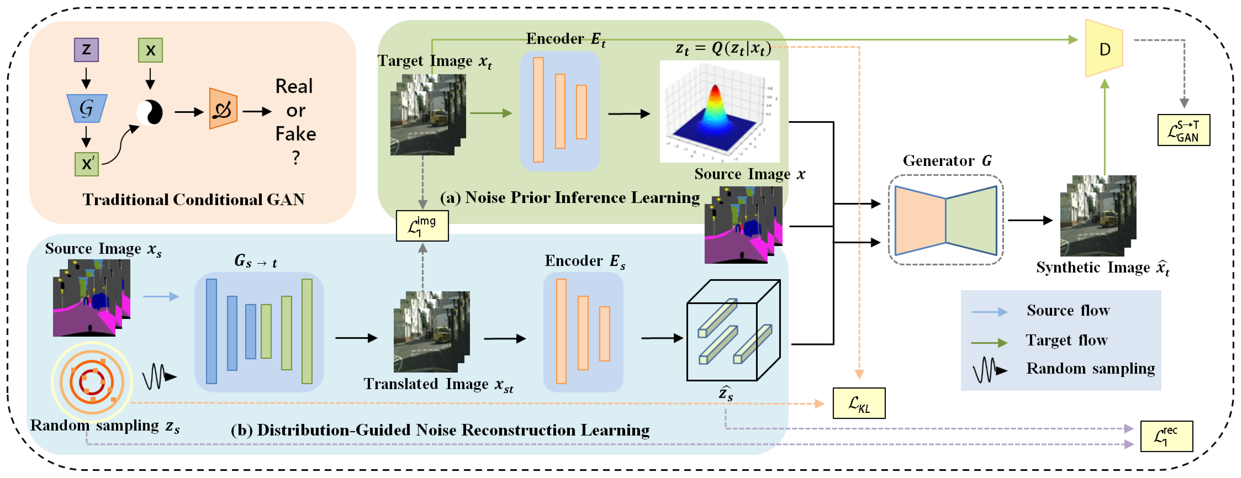
Remotesensing 16 00065 g002
Figure 3. Overall architecture of BnGLGAN. (a) The latent variable z t is inferred from the target domain image x t , the inferred variable z t is used to guide the generation of the conditional GAN, (b) the randomly sampled noise z s is reconstructed to contain source distribution information, and z s is also fed into the generator G. The blue, red, and irregular polyline arrows indicates the source data flow, target data flow, and random sampling, respectively. The dashed lines indicate different kinds of losses.
Remotesensing 16 00065 g003
Figure 4. Structure of (a) variational autoencoder and (b) conditional variational autoencoder.
Remotesensing 16 00065 g004
Figure 5. Some annotated legends of the Cityscapes dataset are presented.
Remotesensing 16 00065 g005
Figure 6. Visual results comparison with several state-of-the-art methods on three benchmark datasets. In the edge-to-shoes and edge-to-handbag translation tasks, this paper uses bidirectional translation for comparison.
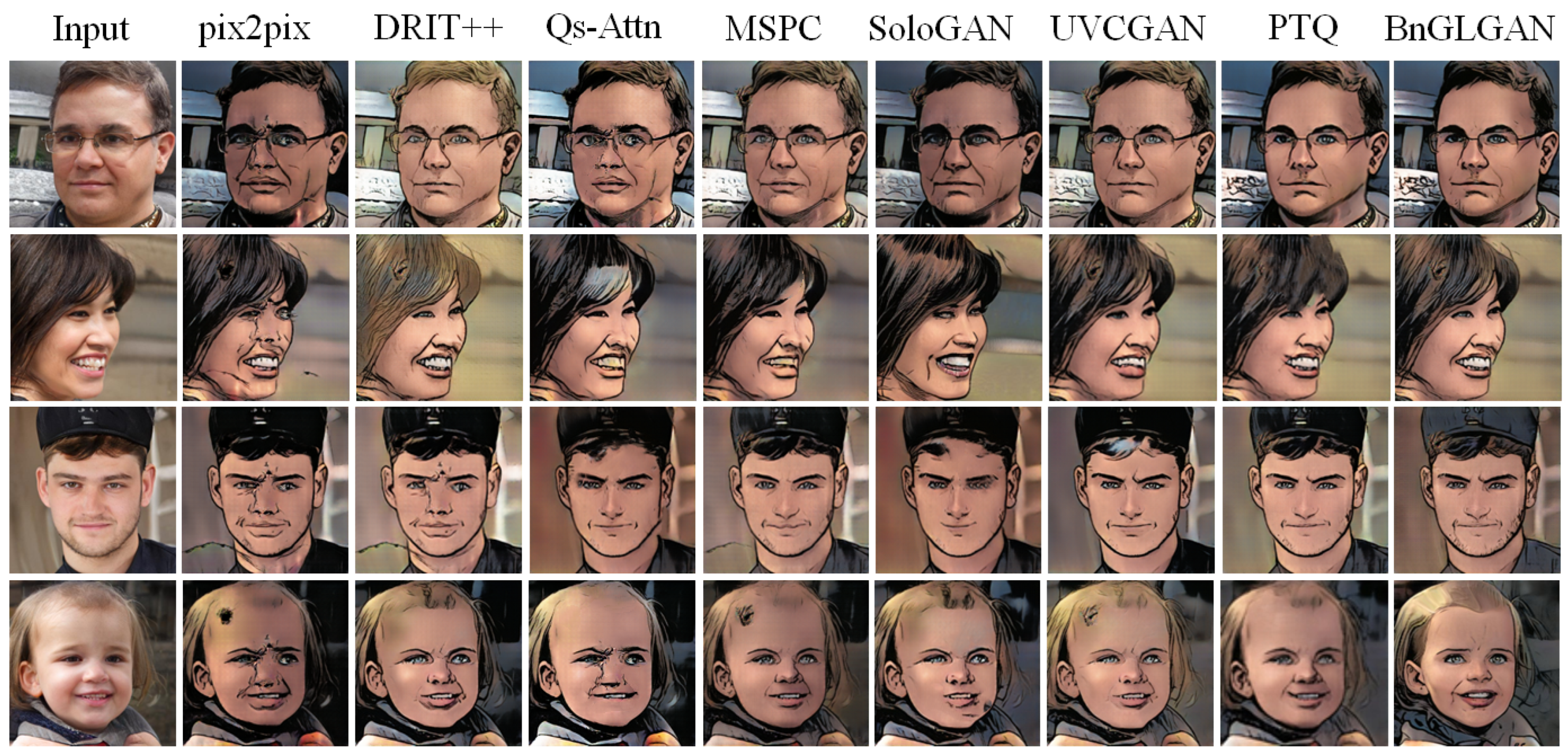
Remotesensing 16 00065 g006
Figure 7. Visual comparison of results of several state-of-the-art methods on facial datasets.
Remotesensing 16 00065 g007
Figure 8. Qualitative comparison of results with other image translation methods. The yellow box shows details of the images recovered by each method. it can be seen that the details generated by BnGLGAN are the most accurate.
Remotesensing 16 00065 g008
Figure 9. Image translation of each method on the night2day dataset. The first two lines show bidirectional image translation, and the last two lines show image translation of other styles of images.
Remotesensing 16 00065 g009
Figure 10. Results of various methods in Maps → Satellite translation task on Google Maps dataset.
Remotesensing 16 00065 g010
Figure 11. Visualization of different I2IT translation tasks using learned attention maps. Each example shows a ground truth image (left) and the corresponding attention map (right).
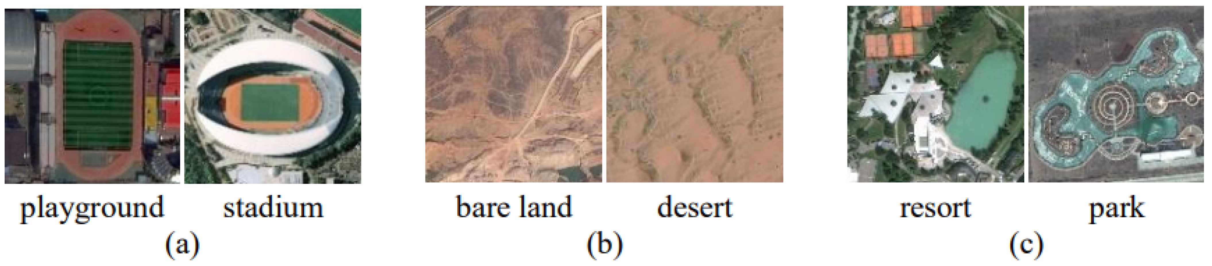
Remotesensing 16 00065 g011
Figure 12. Large intra-class diversity: (a), images of the same setting in multiple dimensions; (b), different styles of buildings in the same setting; (c), diverse imaging conditions of the same setting.
Remotesensing 16 00065 g012
Figure 13. Small inter-class distance: (a), similar objects between different scenes; (b), similar grain between different settings; (c), similar structural distributions between different settings.
Remotesensing 16 00065 g013
Table 1. Details of datasets and settings used in the experiment.
CityscapesFace2comicsCMP FacadesGoogle MapsNight2dayShoesHandbag
# total images (image pairs)347520,000506219420,11050,025138,767
# training images (image pairs)297515,000400109617,82349,82513,8567
# testing images (image pairs)500500010610982287200200
image crop size1024 × 1024512 × 512256 × 256600 × 600256 × 256256 × 256256 × 256
# training epochs3004004004002006060
Table 2. Quantitative performance in image-to-image translation tasks on Cityscapes. The lower the FID and LPIPS, the better the effect.
MethodFID ↓Per-Class Acc.MIoUPSNRSSIMLPIPS ↓
pix2pix [1]61.225.58.4115.1930.2790.379
DRIT++ [32]57.425.711.6015.2300.2870.384
LSCA [50]45.529.127.3315.5650.3690.325
MSPC [51]39.129.633.6715.8310.4250.397
Qs-Attn [52]48.832.637.4516.2350.4010.334
UVCGAN [53]54.733.040.1616.3330.5240.351
PTQ [55]37.634.241.4716.7390.5320.322
BnGLGAN (512 × 512)35.935.642.6016.8390.5470.319
BnGLGAN (1024 × 1024)36.335.644.3016.8430.5500.321
Table 3. Comparison of the time consumption (in seconds) of different models at different resolutions (512 × 512, 1024 × 1024). Each result is the average of 50 tests.
Method512 × 5121024 × 1024MOSB
cycleGAN0.3250.5622.2951.6 GB
pix2pix0.2930.4852.3311.6 GB
DRIT++0.3360.5122.3721.6 GB
LSCA0.3010.4992.4621.8 GB
BnGLGAN0.2870.4312.6571.6 GB
Table 4. Quantitative performance in image-to-image translation task on three edge datasets. The lower the FID and LPIPS, the better the effect.
MethodFace2comicsEdges2shoesEdges2handbag
FID↓SSIMLPIPS↓FID↓SSIMLPIPS↓FID↓SSIMLPIPS↓
pix2pix [1]49.960.2980.28266.690.6250.59843.020.7360.286
DRIT++ [32]28.870.2870.28553.370.6920.49843.670.6880.411
Qs-Attn [52]31.280.2830.24747.10-0.24437.300.682-
MSPC [51]-0.360-34.600.6820.240-0.741-
SoloGAN [56]-0.450-37.940.6910.23433.200.7710.265
UVCGAN [53]32.400.5360.217-0.6840.24635.94-0.244
PTQ [55]30.940.5840.21025.360.7320.23129.670.8010.254
BnGLGAN (Ours)27.390.5860.20521.070.7820.22828.350.7930.182
Table 5. Quantitative performance in various image-to-image translation tasks. The lower the FID and LPIPS, the better the effect.
MethodFacadesGoogle MapsNight2day
FID↓SSIMLPIPS↓FID↓SSIMLPIPS↓FID↓SSIMLPIPS↓
pix2pix [1]96.10.3650.438140.10.1770.321121.20.4410.433
CHAN [57]93.70.3870.422131.50.1870.287117.90.5580.303
Qs-Attn [52]90.20.4170.399129.70.1910.30999.9-0.287
SISM [54]91.70.4220.401110.40.1960.294-0.668-
MSPC [51]87.30.5010.384104.30.2030.31191.20.6540.246
LSCA [50]88.00.4340.35999.80.2120.283-0.659-
UVCGAN [53]85.30.4590.344101.10.2160.29789.80.7010.223
BnGLGAN (Ours)81.20.4880.33591.20.2330.29885.50.6700.214
Table 6. Ablation study on the modules of our proposed method on Cityscapes dataset.
MethodFID ↓SSIMLPIPS ↓
Baseline39.00.4780.336
Baseline + NPIL37.60.5140.329
Baseline + DgNRL37.10.5230.324
Baseline + NPIL + DgNRL (Ours)36.30.5500.321
Disclaimer/Publisher’s Note: The statements, opinions and data contained in all publications are solely those of the individual author(s) and contributor(s) and not of MDPI and/or the editor(s). MDPI and/or the editor(s) disclaim responsibility for any injury to people or property resulting from any ideas, methods, instructions or products referred to in the content.

