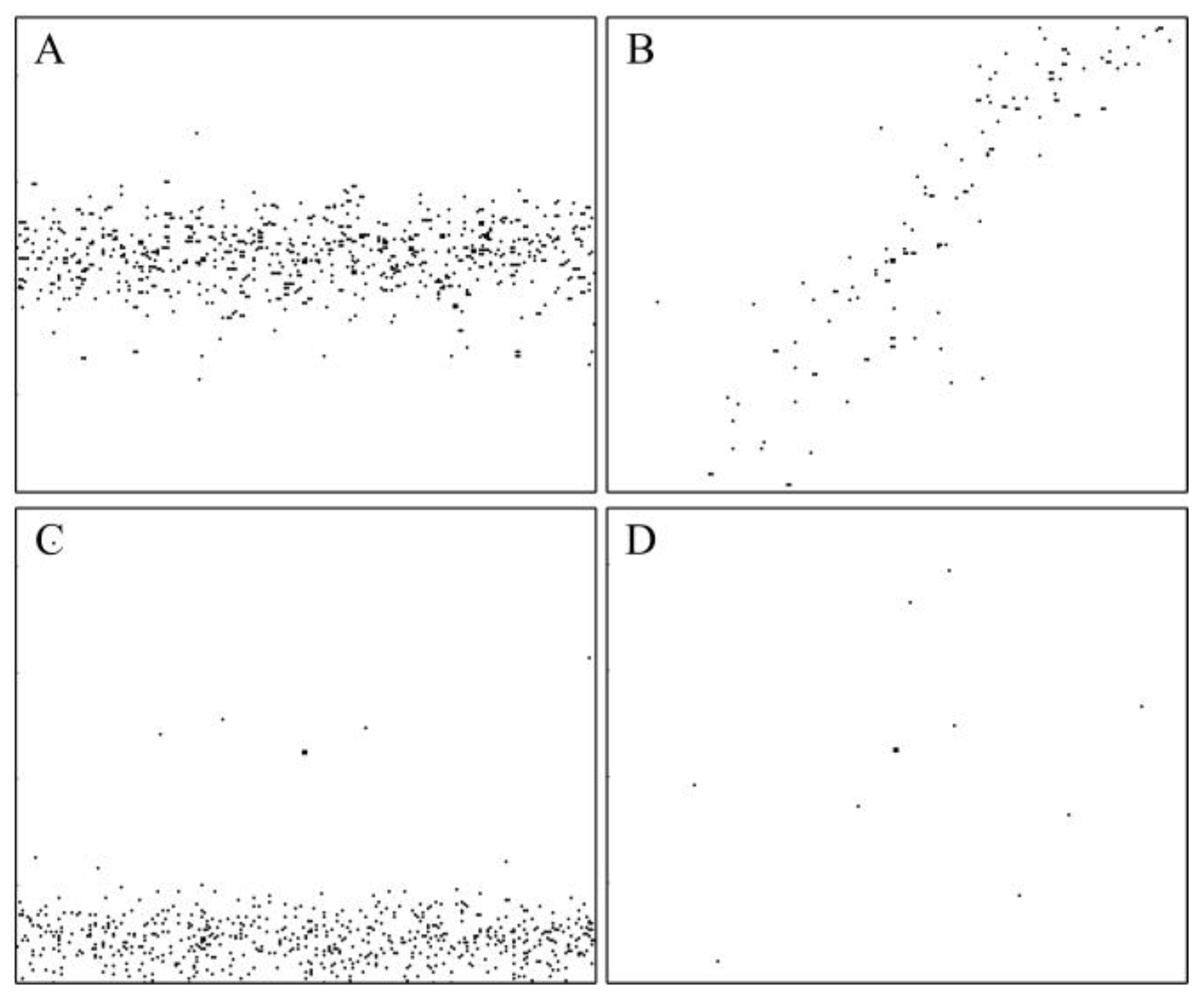
Figure 1.
Overview of the experimental areas A, B, C and D.
Figure 1.
Overview of the experimental areas A, B, C and D.
Figure 2.
Method flow chart.
Figure 2.
Method flow chart.
Figure 3.
Schematic diagram of the photon transformation process.
Figure 3.
Schematic diagram of the photon transformation process.
Figure 4.
Schematic diagram of the Inception module [
39].
Figure 4.
Schematic diagram of the Inception module [
39].
Figure 5.
Schematic diagram of the CAM module [
35].
Figure 5.
Schematic diagram of the CAM module [
35].
Figure 6.
Schematic diagram of the SAM module [
35].
Figure 6.
Schematic diagram of the SAM module [
35].
Figure 7.
The training process of network model in experimental areas A and B. (a) Change curve of accuracy; (b) change curve of loss.
Figure 7.
The training process of network model in experimental areas A and B. (a) Change curve of accuracy; (b) change curve of loss.
Figure 8.
The training process of the network model in experimental area C. (a) Change curve of accuracy; (b) change curve of loss.
Figure 8.
The training process of the network model in experimental area C. (a) Change curve of accuracy; (b) change curve of loss.
Figure 9.
Typical photon neighborhood of photon A, B, C and D and comparison of denoised results. (a) The denoised result of the proposed method (SNR = 80 dB); (b) the denoised result of DBSCAN (SNR = 80 dB); (c) validation.
Figure 9.
Typical photon neighborhood of photon A, B, C and D and comparison of denoised results. (a) The denoised result of the proposed method (SNR = 80 dB); (b) the denoised result of DBSCAN (SNR = 80 dB); (c) validation.
Figure 10.
Photon images of typical photons A, B, C, and D in
Figure 9.
Figure 10.
Photon images of typical photons A, B, C, and D in
Figure 9.
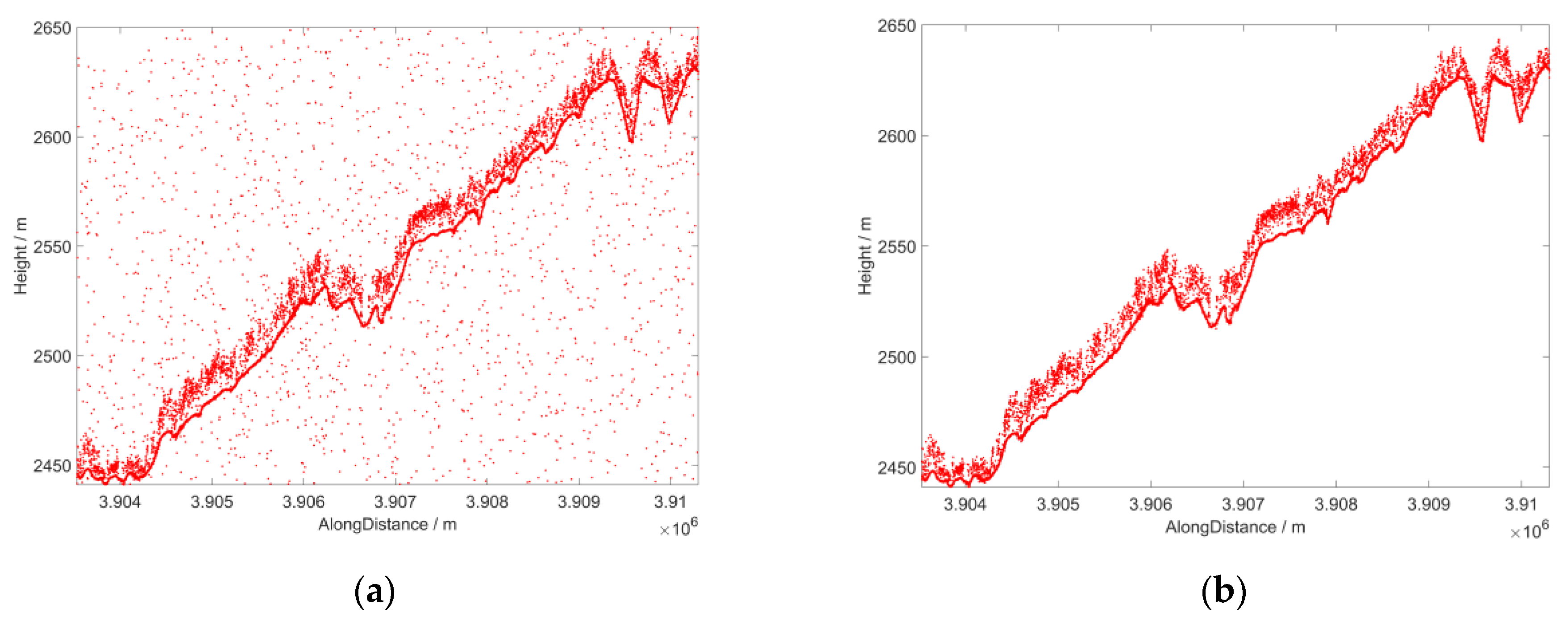
Figure 11.
Overall distribution of photon data in experimental area A. (a) Original photon data; (b) signal photon data.
Figure 11.
Overall distribution of photon data in experimental area A. (a) Original photon data; (b) signal photon data.
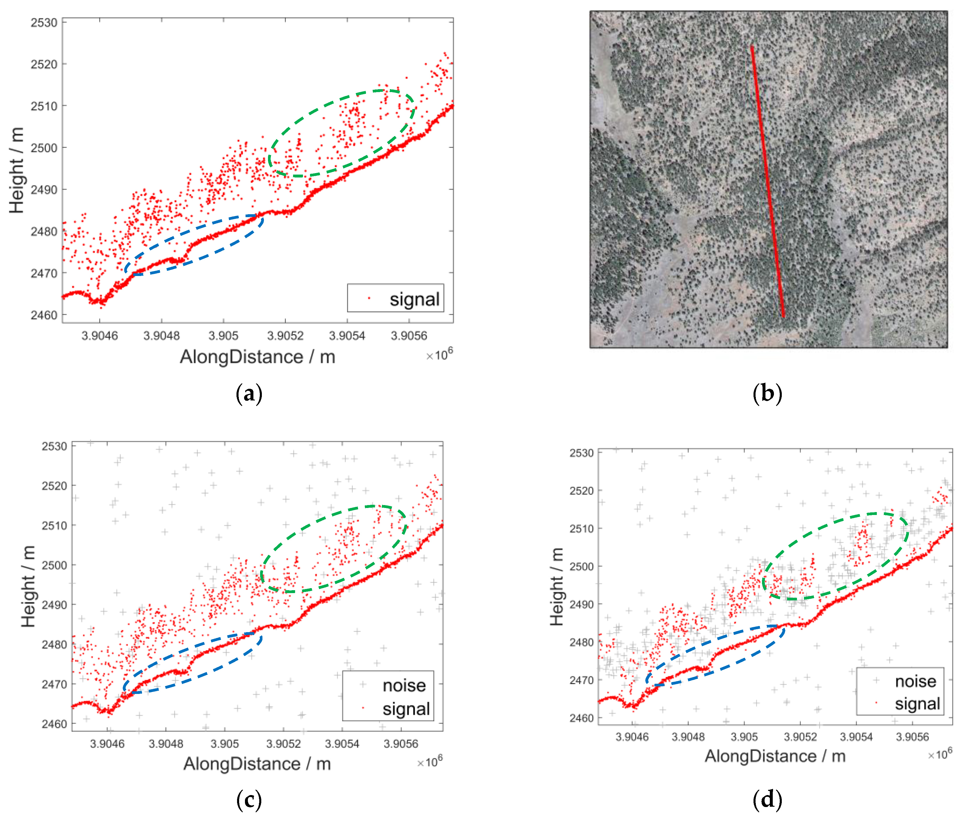
Figure 12.
Comparison of the details of the gt2L track results in the experimental area A (SNR = 70 dB). (a) validation; (b) optical remote sensing image; (c) the proposed method; (d) DBSCAN; (e) OPTICS; (f) BED.
Figure 12.
Comparison of the details of the gt2L track results in the experimental area A (SNR = 70 dB). (a) validation; (b) optical remote sensing image; (c) the proposed method; (d) DBSCAN; (e) OPTICS; (f) BED.
Figure 13.
Curves of change in four validation indicators with SNR in experimental area A. (a) Precision; (b) Recall; (c) OA; (d) Kappa.
Figure 13.
Curves of change in four validation indicators with SNR in experimental area A. (a) Precision; (b) Recall; (c) OA; (d) Kappa.
Figure 14.
Overall distribution of photon data in experimental area B. (a) Original photon data; (b) signal photon data.
Figure 14.
Overall distribution of photon data in experimental area B. (a) Original photon data; (b) signal photon data.
Figure 15.
Comparison of the details of the results of the gt2R track in experimental area B (SNR = 70 dB). (a) Validation; (b) optical remote sensing image; (c) the proposed method; (d) DBSCAN; (e) OPTICS; (f) BED.
Figure 15.
Comparison of the details of the results of the gt2R track in experimental area B (SNR = 70 dB). (a) Validation; (b) optical remote sensing image; (c) the proposed method; (d) DBSCAN; (e) OPTICS; (f) BED.
Figure 16.
Curves of change in four validation indicators with SNR in experimental area B. (a) Precision; (b) Recall; (c) OA; (d) Kappa.
Figure 16.
Curves of change in four validation indicators with SNR in experimental area B. (a) Precision; (b) Recall; (c) OA; (d) Kappa.
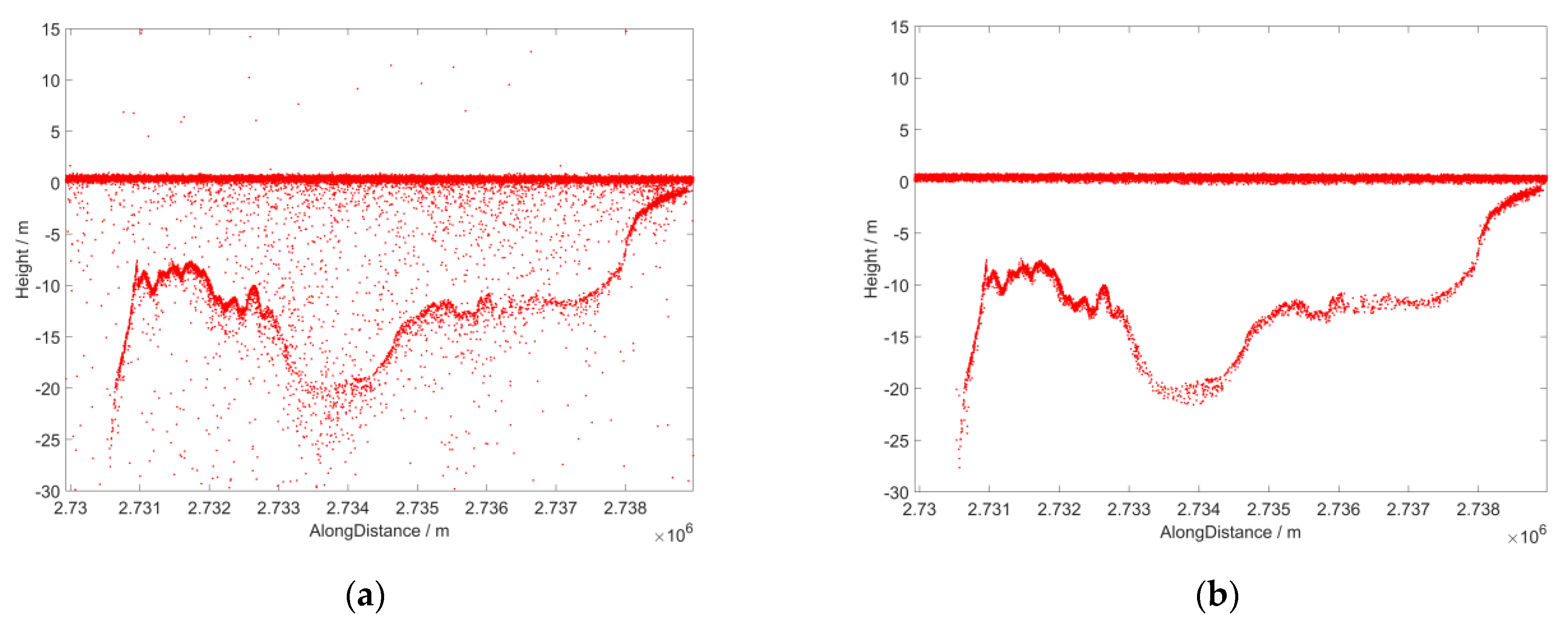
Figure 17.
Overall distribution of photon data in experimental area C. (a) Original photon data; (b) signal photon data.
Figure 17.
Overall distribution of photon data in experimental area C. (a) Original photon data; (b) signal photon data.
Figure 18.
Comparison of the details of the gt3L track results in experimental area C (SNR = 80 dB). (a) Validation; (b) optical remote sensing image; (c) the proposed method; (d) DBSCAN; (e) OPTICS; (f) BED.
Figure 18.
Comparison of the details of the gt3L track results in experimental area C (SNR = 80 dB). (a) Validation; (b) optical remote sensing image; (c) the proposed method; (d) DBSCAN; (e) OPTICS; (f) BED.
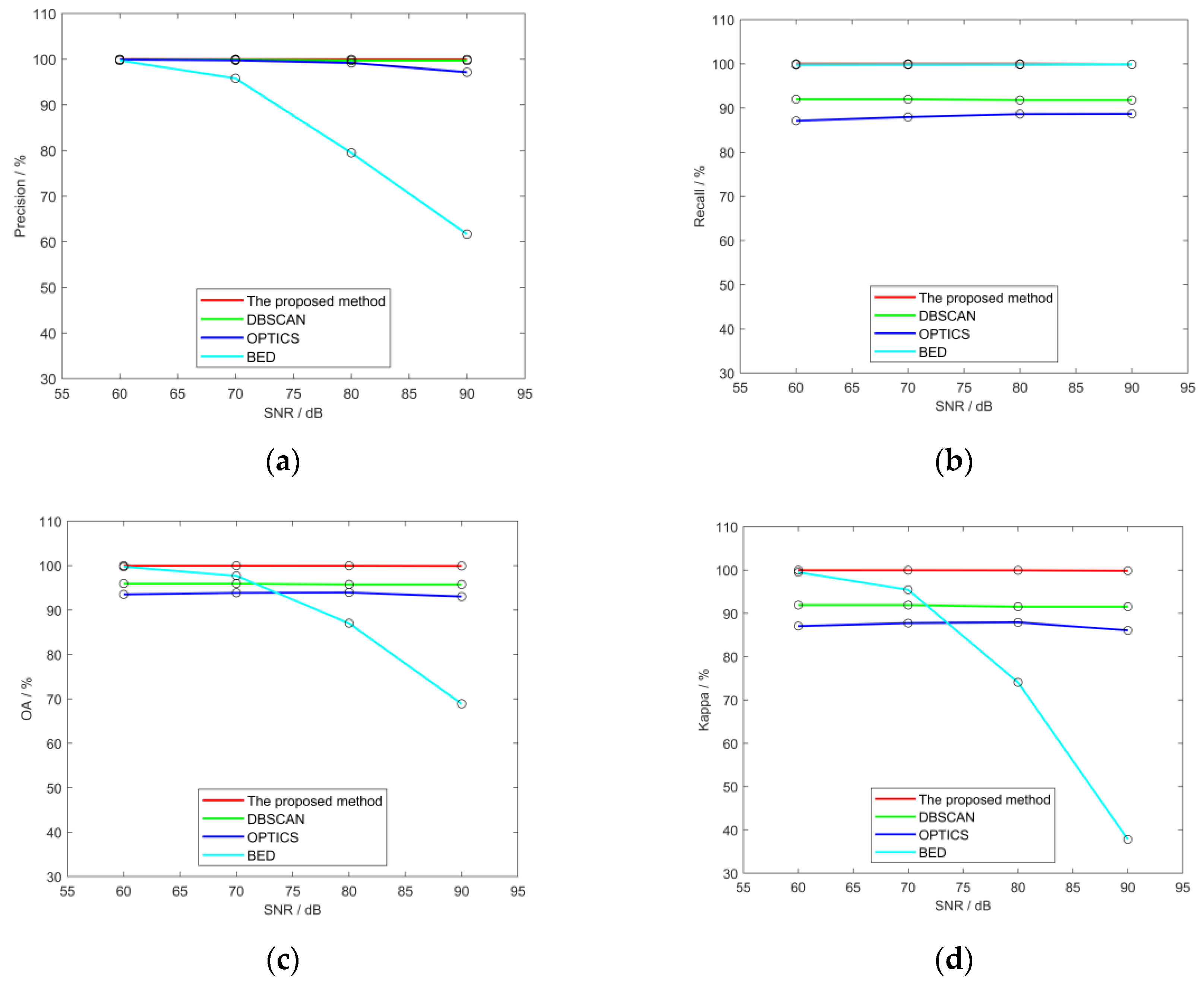
Figure 19.
Curves of change in four validation indicators with SNR in experimental area C. (a) Precision; (b) Recall; (c) OA; (d) Kappa.
Figure 19.
Curves of change in four validation indicators with SNR in experimental area C. (a) Precision; (b) Recall; (c) OA; (d) Kappa.
Figure 20.
Overall distribution of photon data in experimental area D. (a) Original photon data; (b) signal photon data.
Figure 20.
Overall distribution of photon data in experimental area D. (a) Original photon data; (b) signal photon data.
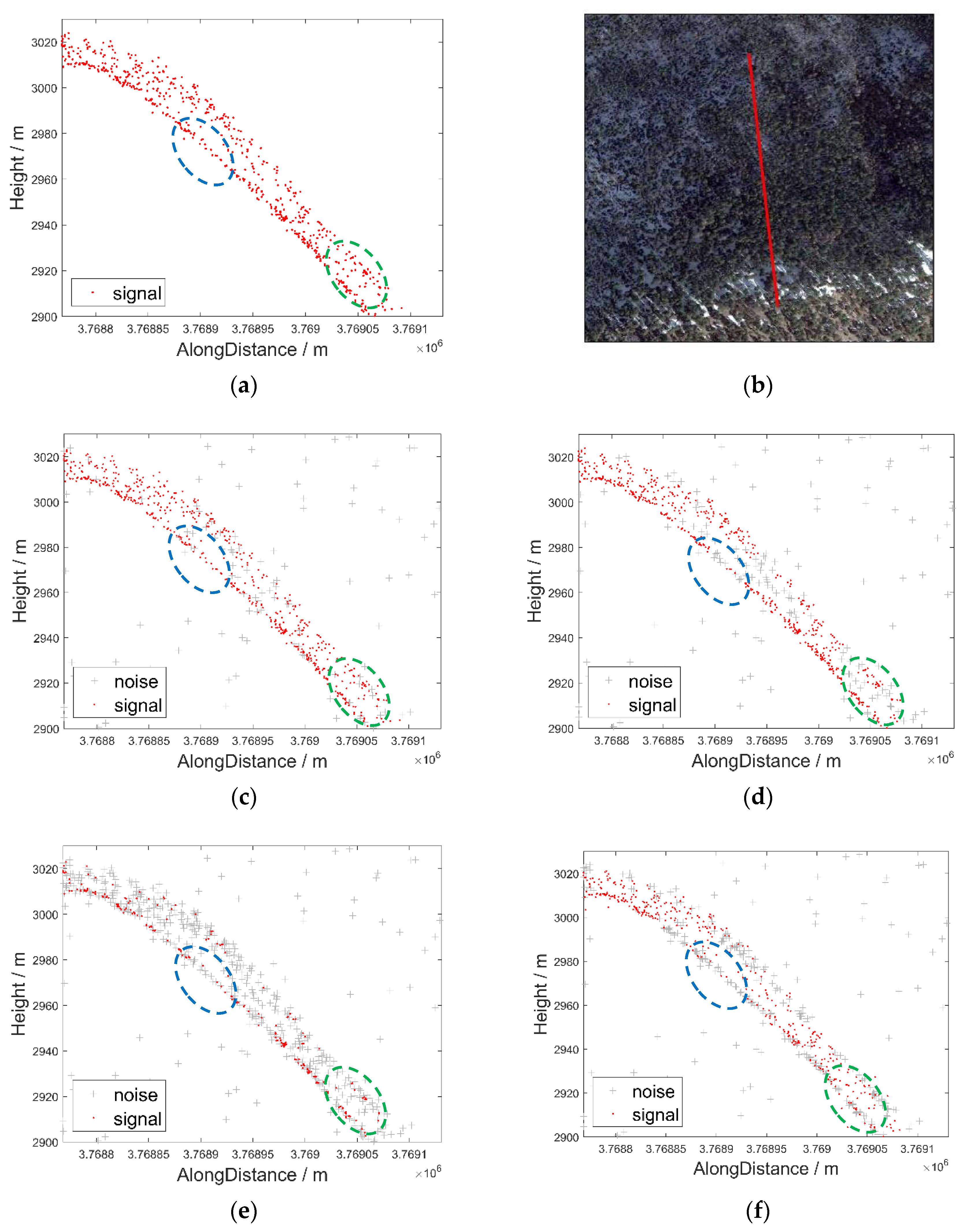
Figure 21.
Comparison of the details of the gt2R track results in experimental area D (SNR = 80 dB). (a) Validation; (b) optical remote sensing image; (c) the proposed method; (d) DBSCAN; (e) OPTICS; (f) BED.
Figure 21.
Comparison of the details of the gt2R track results in experimental area D (SNR = 80 dB). (a) Validation; (b) optical remote sensing image; (c) the proposed method; (d) DBSCAN; (e) OPTICS; (f) BED.
Figure 22.
Curves of change in four validation indicators with SNR in experimental area D. (a) Precision; (b) Recall; (c) OA; (d) Kappa.
Figure 22.
Curves of change in four validation indicators with SNR in experimental area D. (a) Precision; (b) Recall; (c) OA; (d) Kappa.
Figure 23.
Schematic of real reference verification in experimental area A. (a) Scatterplot of elevation and actual elevation of gt2R track signal photons in experimental area A; (b) track distribution diagram in experimental area A.
Figure 23.
Schematic of real reference verification in experimental area A. (a) Scatterplot of elevation and actual elevation of gt2R track signal photons in experimental area A; (b) track distribution diagram in experimental area A.
Figure 24.
Schematic of real reference verification in experimental area B. (a) Scatterplot of elevation and actual elevation of gt1R track signal photons in the experimental area B; (b) track distribution diagram in the experimental area B.
Figure 24.
Schematic of real reference verification in experimental area B. (a) Scatterplot of elevation and actual elevation of gt1R track signal photons in the experimental area B; (b) track distribution diagram in the experimental area B.
Figure 25.
Schematic of real reference verification in experimental area C. (a) Scatterplot of elevation and actual elevation of gt3L track signal photons in experimental area C; (b) track distribution diagram in experimental area C.
Figure 25.
Schematic of real reference verification in experimental area C. (a) Scatterplot of elevation and actual elevation of gt3L track signal photons in experimental area C; (b) track distribution diagram in experimental area C.
Figure 26.
Schematic of real reference verification in experimental area D. (a) Scatterplot of elevation and actual elevation of gt2R track signal photons in experimental area D; (b) track distribution diagram in experimental area D.
Figure 26.
Schematic of real reference verification in experimental area D. (a) Scatterplot of elevation and actual elevation of gt2R track signal photons in experimental area D; (b) track distribution diagram in experimental area D.
Table 1.
Information on ICESat-2/ATL03 data used.
Table 1.
Information on ICESat-2/ATL03 data used.
| Experimental Area | ICESat-2/ATL03 | Data Acquisition Time | Track Used |
|---|
| A | ATL03_20200914131032_12400802_005_01.h5 | 14 September 2020
14:13:10 | gt1L/gt2L/gt3L |
| B | ATL03_20191114034331_07370502_005_01.h5 | 14 November 2019
3:43:31 | gt1R/gt2R/gt3R |
| C | ATL03_20190807063856_06140401_005_01.h5 | 7 August 2019
6:28:56 | gt1L/gt2L/gt3L |
| D | ATL03_20221111233317_07981702_006_01.h5 | 11 November 2022
23:33:17 | gt1R/gt2R/gt3R |
Table 2.
Information about the training hyperparameters.
Table 2.
Information about the training hyperparameters.
| Training Hyperparameter | Setting |
|---|
| Initial learning rate | 0.001 |
| Learning rate change modality | ExponentialLR |
| Learning rate change rate | 0.98 |
| Batch size | 2 |
| Optimizer | adam |
| Training epoch | 20 |
| Training to validation | 8:2 |
Table 3.
Results of the gt2L track in experimental area A.
Table 3.
Results of the gt2L track in experimental area A.
| | SNR (dB) | Precision | Recall | OA | Kappa |
|---|
| The proposed method | 60 | 99.97% | 98.96% | 99.47% | 98.93% |
| 70 | 99.94% | 98.94% | 99.44% | 98.88% |
| 80 | 99.82% | 98.89% | 99.35% | 98.71% |
| 90 | 99.50% | 98.72% | 99.11% | 98.22% |
| DBSCAN | 60 | 99.69% | 91.59% | 95.65% | 91.30% |
| 70 | 98.95% | 93.14% | 96.08% | 92.15% |
| 80 | 95.72% | 94.15% | 94.97% | 89.94% |
| 90 | 82.82% | 97.62% | 88.68% | 77.37% |
| OPTICS | 60 | 99.84% | 50.54% | 75.23% | 50.46% |
| 70 | 98.95% | 72.13% | 85.68% | 71.36% |
| 80 | 98.47% | 72.81% | 85.84% | 71.68% |
| 90 | 93.44% | 75.33% | 85.02% | 70.04% |
| BED | 60 | 99.63% | 82.85% | 91.27% | 82.54% |
| 70 | 98.62% | 83.35% | 91.09% | 82.19% |
| 80 | 95.02% | 84.58% | 90.07% | 80.14% |
| 90 | 80.85% | 88.14% | 83.63% | 67.27% |
Table 4.
Results of the gt2R track in experimental area B.
Table 4.
Results of the gt2R track in experimental area B.
| | SNR (dB) | Precision | Recall | OA | Kappa |
|---|
| The proposed method | 60 | 99.98% | 97.63% | 98.81% | 97.62% |
| 70 | 99.90% | 97.56% | 98.74% | 97.48% |
| 80 | 99.70% | 97.48% | 98.60% | 97.20% |
| 90 | 99.33% | 97.26% | 98.31% | 96.63% |
| DBSCAN | 60 | 98.51% | 92.95% | 95.82% | 91.64% |
| 70 | 98.63% | 93.12% | 95.96% | 91.92% |
| 80 | 94.61% | 96.25% | 95.44% | 90.87% |
| 90 | 81.80% | 97.99% | 88.24% | 76.47% |
| OPTICS | 60 | 99.51% | 37.82% | 69.18% | 38.36% |
| 70 | 98.56% | 57.42% | 78.54% | 57.08% |
| 80 | 94.40% | 72.14% | 84.12% | 68.23% |
| 90 | 89.07% | 78.56% | 84.64% | 69.28% |
| BED | 60 | 99.31% | 74.88% | 87.33% | 74.65% |
| 70 | 97.72% | 75.55% | 87.05% | 74.09% |
| 80 | 91.60% | 77.70% | 85.46% | 70.92% |
| 90 | 74.16% | 83.17% | 77.37% | 54.73% |
Table 5.
Results of the gt3L track in experimental area C.
Table 5.
Results of the gt3L track in experimental area C.
| | SNR (dB) | Precision | Recall | OA | Kappa |
|---|
| The proposed method | 60 | 99.99% | 99.98% | 99.99% | 99.98% |
| 70 | 99.99% | 99.98% | 99.99% | 99.97% |
| 80 | 99.97% | 99.98% | 99.97% | 99.95% |
| 90 | 99.96% | 99.89% | 99.93% | 99.85% |
| DBSCAN | 60 | 99.93% | 91.99% | 95.96% | 91.93% |
| 70 | 99.93% | 91.99% | 95.96% | 91.93% |
| 80 | 99.71% | 91.81% | 95.77% | 91.54% |
| 90 | 99.71% | 91.81% | 95.77% | 91.54% |
| OPTICS | 60 | 99.95% | 87.12% | 93.53% | 87.07% |
| 70 | 99.76% | 87.97% | 93.88% | 87.76% |
| 80 | 99.20% | 88.64% | 93.96% | 87.93% |
| 90 | 97.15% | 88.69% | 93.04% | 86.08% |
| BED | 60 | 99.72% | 99.78% | 99.75% | 99.50% |
| 70 | 95.81% | 99.81% | 97.72% | 95.45% |
| 80 | 79.49% | 99.83% | 87.03% | 74.07% |
| 90 | 61.67% | 99.90% | 68.90% | 37.81% |
Table 6.
Results of the gt2R track in the experimental area D.
Table 6.
Results of the gt2R track in the experimental area D.
| | SNR (dB) | Precision | Recall | OA | Kappa |
|---|
| The proposed method | 60 | 99.89% | 99.84% | 99.87% | 99.73% |
| 70 | 99.97% | 99.84% | 99.91% | 99.81% |
| 80 | 99.67% | 99.82% | 99.75% | 99.49% |
| 90 | 99.68% | 99.81% | 99.75% | 99.49% |
| DBSCAN | 60 | 98.88% | 99.98% | 99.43% | 98.85% |
| 70 | 99.63% | 99.88% | 99.75% | 99.50% |
| 80 | 95.03% | 99.99% | 97.39% | 94.77% |
| 90 | 94.66% | 99.99% | 97.18% | 94.36% |
| OPTICS | 60 | 99.63% | 96.34% | 97.99% | 95.97% |
| 70 | 99.91% | 93.91% | 96.92% | 93.83% |
| 80 | 98.44% | 96.77% | 97.62% | 95.24% |
| 90 | 98.28% | 97.08% | 97.69% | 95.38% |
| BED | 60 | 96.53% | 99.60% | 98.01% | 96.01% |
| 70 | 99.54% | 99.50% | 99.52% | 99.05% |
| 80 | 97.22% | 98.91% | 98.04% | 96.09% |
| 90 | 97.07% | 98.75% | 97.88% | 95.77% |
Table 7.
Accuracy results within different elevation intervals of the gt2R track in experimental area A (The best result for each evaluation interval is bolded).
Table 7.
Accuracy results within different elevation intervals of the gt2R track in experimental area A (The best result for each evaluation interval is bolded).
| | RMSE | MAE | MRE | Range |
|---|
| The proposed method | 1.36 | 0.79 | 0.03% | 2319.22–2404.32 m |
| 4.34 | 1.09 | 0.04% | 2404.32–2489.43 m |
| 1.93 | 0.79 | 0.03% | 2489.43–2574.54 m |
| 4.12 | 0.64 | 0.02% | 2574.54–2659.64 m |
| 3.40 | 0.75 | 0.03% | Overall |
| DBSCAN | 3.64 | 1.10 | 0.05% | 2319.22–2404.32 m |
| 3.09 | 1.26 | 0.05% | 2404.32–2489.43 m |
| 4.25 | 1.09 | 0.04% | 2489.43–2574.54 m |
| 3.34 | 0.89 | 0.03% | 2574.54–2659.64 m |
| 3.58 | 1.09 | 0.04% | Overall |
| OPTICS | 3.93 | 0.75 | 0.03% | 2319.22–2404.32 m |
| 6.63 | 1.17 | 0.05% | 2404.32–2489.43 m |
| 4.18 | 0.88 | 0.03% | 2489.43–2574.54 m |
| 4.66 | 0.68 | 0.03% | 2574.54–2659.64 m |
| 4.85 | 0.87 | 0.03% | Overall |
| BED | 15.99 | 7.81 | 0.33% | 2319.22–2404.32 m |
| 22.85 | 11.36 | 0.46% | 2404.32–2489.43 m |
| 19.07 | 8.66 | 0.34% | 2489.43–2574.54 m |
| 20.38 | 12.34 | 0.47% | 2574.54–2659.64 m |
| 19.57 | 10.04 | 0.40% | Overall |
Table 8.
Accuracy results within different elevation intervals of the gt1R track in the experimental area B (The best result for each evaluation interval is bolded).
Table 8.
Accuracy results within different elevation intervals of the gt1R track in the experimental area B (The best result for each evaluation interval is bolded).
| | RMSE | MAE | MRE | Range |
|---|
| The proposed method | 4.14 | 1.39 | 0.06% | 2361.07–2492.91 m |
| 2.31 | 1.67 | 0.07% | 2492.91–2624.75 m |
| 3.96 | 2.69 | 0.10% | 2624.75–2756.58 m |
| 4.40 | 3.09 | 0.11% | 2756.58–2888.42 m |
| 3.86 | 2.28 | 0.08% | Overall |
| DBSCAN | 3.03 | 1.78 | 0.07% | 2361.07–2492.91 m |
| 4.22 | 2.59 | 0.10% | 2492.91–2624.75 m |
| 6.28 | 4.28 | 0.16% | 2624.75–2756.58 m |
| 6.38 | 4.75 | 0.17% | 2756.58–2888.42 m |
| 4.98 | 3.35 | 0.13% | Overall |
| OPTICS | 10.38 | 2.27 | 0.09% | 2361.07–2492.91 m |
| 12.07 | 3.07 | 0.12% | 2492.91–2624.75 m |
| 10.46 | 3.76 | 0.14% | 2624.75–2756.58 m |
| 9.18 | 4.19 | 0.15% | 2756.58–2888.42 m |
| 10.52 | 3.32 | 0.13% | Overall |
| BED | 15.63 | 3.76 | 0.16% | 2361.07–2492.91 m |
| 16.69 | 4.82 | 0.19% | 2492.91–2624.75 m |
| 14.15 | 5.48 | 0.20% | 2624.75–2756.58 m |
| 14.32 | 6.04 | 0.21% | 2756.58–2888.42 m |
| 15.20 | 5.02 | 0.19% | Overall |
Table 9.
Accuracy results within different elevation intervals of the gt3L track in experimental area C (The best result for each evaluation interval is bolded).
Table 9.
Accuracy results within different elevation intervals of the gt3L track in experimental area C (The best result for each evaluation interval is bolded).
| | RMSE | MAE | MRE | Range |
|---|
| The proposed method | 1.11 | 0.44 | 13.25% | 2–5 m |
| 0.55 | 0.71 | 10.37% | 5–10 m |
| 0.90 | 0.94 | 8.51% | 10–15 m |
| 1.46 | 1.74 | 11.84% | 15–20 m |
| 0.81 | 0.69 | 10.74% | Overall |
| DBSCAN | 0.64 | 0.77 | 26.69% | 2–5 m |
| 0.71 | 0.76 | 10.77% | 5–10 m |
| 0.61 | 1.43 | 16.70% | 10–15 m |
| - | - | - | 15–20 m |
| 0.65 | 0.99 | 18.05% | Overall |
| OPTICS | 0.44 | 0.77 | 29.73% | 2–5 m |
| 0.50 | 0.73 | 10.67% | 5–10 m |
| 0.29 | 1.06 | 12.81% | 10–15 m |
| - | - | - | 15–20 m |
| 0.41 | 0.85 | 17.74% | Overall |
| BED | 2.44 | 1.42 | 29.32% | 2–5 m |
| 0.72 | 0.75 | 10.97% | 5–10 m |
| 1.08 | 1.11 | 10.69% | 10–15 m |
| 0.52 | 2.11 | 15.28% | 15–20 m |
| 1.19 | 1.35 | 16.57% | Overall |
Table 10.
Accuracy results within different elevation intervals of the gt2R track in experimental area D (The best result for each evaluation interval is bolded).
Table 10.
Accuracy results within different elevation intervals of the gt2R track in experimental area D (The best result for each evaluation interval is bolded).
| | RMSE/m | MAE/m | MRE | Range |
|---|
| The proposed method | 3.00 | 2.71 | 0.16% | 1659–1672 m |
| 2.96 | 3.40 | 0.20% | 1672–1685 m |
| 2.95 | 2.80 | 0.17% | 1685–1698 m |
| 3.17 | 9.94 | 0.58% | 1698–1711 m |
| 3.02 | 4.71 | 0.28% | Overall |
| DBSCAN | 2.95 | 2.71 | 0.16% | 1659–1672 m |
| 2.98 | 3.45 | 0.21% | 1672–1685 m |
| 2.96 | 2.81 | 0.17% | 1685–1698 m |
| 3.16 | 9.92 | 0.58% | 1698–1711 m |
| 3.01 | 4.72 | 0.28% | Overall |
| OPTICS | 2.79 | 2.61 | 0.16% | 1659–1672 m |
| 2.99 | 3.30 | 0.20% | 1672–1685 m |
| 2.93 | 2.79 | 0.17% | 1685–1698 m |
| 3.21 | 10.27 | 0.60% | 1698–1711 m |
| 2.98 | 4.75 | 0.28% | Overall |
| BED | 3.09 | 2.75 | 0.17% | 1659–1672 m |
| 2.97 | 3.42 | 0.20% | 1672–1685 m |
| 2.95 | 2.80 | 0.17% | 1685–1698 m |
| 3.16 | 9.93 | 0.58% | 1698–1711 m |
| 3.04 | 4.73 | 0.28% | Overall |
Table 11.
Comparison of results between different CNN models (The best result for each evaluation interval is bolded).
Table 11.
Comparison of results between different CNN models (The best result for each evaluation interval is bolded).
| Name | SNR (dB) | Precision | Recall | OA | Kappa |
|---|
| DenseNet201 | 60 | 99.66% | 97.67% | 98.67% | 97.35% |
| 70 | 99.15% | 97.00% | 98.09% | 96.18% |
| 80 | 98.99% | 96.66% | 97.84% | 95.67% |
| 90 | 98.33% | 92.62% | 95.54% | 91.09% |
| Average | 99.03% | 95.99% | 97.54% | 95.07% |
| GoogLeNet | 60 | 99.72% | 98.45% | 99.09% | 98.18% |
| 70 | 99.27% | 98.37% | 98.83% | 97.66% |
| 80 | 98.87% | 98.48% | 98.68% | 97.36% |
| 90 | 97.90% | 97.96% | 97.93% | 95.87% |
| Average | 98.94% | 98.32% | 98.63% | 97.27% |
| ResNet18 | 60 | 99.50% | 97.56% | 98.54% | 97.07% |
| 70 | 98.72% | 97.03% | 97.89% | 95.78% |
| 80 | 98.24% | 96.93% | 97.60% | 95.20% |
| 90 | 97.35% | 94.57% | 96.00% | 92.01% |
| Average | 98.45% | 96.52% | 97.51% | 95.02% |
| ResNet50 | 60 | 99.94% | 94.87% | 97.41% | 94.82% |
| 70 | 99.86% | 93.57% | 96.72% | 93.45% |
| 80 | 99.77% | 93.86% | 96.83% | 93.67% |
| 90 | 99.65% | 87.21% | 93.47% | 86.95% |
| Average | 99.80% | 92.38% | 96.11% | 92.22% |
| VGG16 | 60 | 99.69% | 98.43% | 99.06% | 98.13% |
| 70 | 99.23% | 98.05% | 98.65% | 97.30% |
| 80 | 98.72% | 98.12% | 98.43% | 96.85% |
| 90 | 97.98% | 95.52% | 96.79% | 93.57% |
| Average | 98.90% | 97.53% | 98.23% | 96.46% |
Table 12.
Comparison of the accuracy of results before and after using CBAM (The best result for each evaluation interval is bolded).
Table 12.
Comparison of the accuracy of results before and after using CBAM (The best result for each evaluation interval is bolded).
| Name | SNR (dB) | Precision | Recall | OA | Kappa |
|---|
| GoogLeNet | 60 | 99.72% | 98.45% | 99.09% | 98.18% |
| 70 | 99.27% | 98.37% | 98.83% | 97.66% |
| 80 | 98.87% | 98.48% | 98.68% | 97.36% |
| 90 | 97.90% | 97.96% | 97.93% | 95.87% |
| Average | 98.94% | 98.32% | 98.63% | 97.27% |
| GoogLeNet + CBAM | 60 | 99.94% | 98.75% | 99.34% | 98.69% |
| 70 | 99.86% | 98.69% | 99.28% | 98.56% |
| 80 | 99.67% | 98.58% | 99.13% | 98.26% |
| 90 | 99.43% | 98.40% | 98.92% | 97.84% |
| Average | 99.72% | 98.60% | 99.17% | 98.33% |


