Article

Exploration of Data Scene Characterization and 3D ROC Evaluation for Hyperspectral Anomaly Detection

1
Center for Hyperspectral Imaging in Remote Sensing (CHIRS), Information and Technology College, Dalian Maritime University, Dalian 116026, China
2
Remote Sensing Signal and Image Processing Laboratory, Department of Computer Science and Electrical Engineering, University of Maryland, Baltimore County, Baltimore, MD 21250, USA
3
Department of Electrical Engineering, National Cheng Kung University, Tainan 70101, Taiwan
4
Department of Electrical Engineering, Zhejiang University, Hangzhou 310027, China
5
School of Computer Science and Engineering, Nanjing University of Science and Technology, Nanjing 210094, China
*
Author to whom correspondence should be addressed.
Remote Sens. 2024, 16(1), 135; https://doi.org/10.3390/rs16010135
Submission received: 5 November 2023 / Revised: 16 December 2023 / Accepted: 21 December 2023 / Published: 28 December 2023
(This article belongs to the Special Issue Advances in Hyperspectral Data Exploitation II)

Abstract

:
Whether or not a hyperspectral anomaly detector is effective is determined by two crucial issues, anomaly detectability and background suppressibility (BS), both of which are very closely related to two factors, the datasets used for a selected hyperspectral anomaly detector and detection measures used for its performance evaluation. This paper explores how anomaly detectability and BS play key roles in hyperspectral anomaly detection (HAD). To address these two issues, we investigate three key elements attributed to HAD. One is a selected hyperspectral anomaly detector, and another is the datasets used for experiments. The third one is the detection measures used to evaluate the effectiveness of a hyperspectral anomaly detector. As for hyperspectral anomaly detectors, twelve commonly used anomaly detectors were evaluated and compared. To address the appropriate use of datasets for HAD, seven popular and widely used datasets were studied for HAD. As for the third issue, the traditional area under a receiver operating characteristic (ROC) curve of detection probability—PD versus false alarm probability, PF, (AUC(D,F))—was extended to 3D ROC analysis where a 3D ROC curve was developed to generate three 2D ROC curves from which eight detection measures could be derived to evaluate HAD in all round aspects, including anomaly detectability, BS and joint anomaly detectability and BS. Qualitative analysis showed that many works reported in the literature which claimed that their developed hyperspectral anomaly detectors performed better than other anomaly detectors are actually not true because they overlooked these two issues. Specifically, a comprehensive study via extensive experiments demonstrated that these 3D ROC curve-derived detection measures can be further used to address the various characterizations of different data scenes and also to provide explanations as to why certain data scenes are not suitable for HAD.

1. Introduction

Due to the very fine spectral resolution provided by hundreds of contiguous spectral bands, hyperspectral imaging (HSI) can reveal and uncover many unknown subtle material substances which cannot be identified by prior knowledge or visual inspection [1]. Many of these unidentified substances are generally considered to be anomalies and can provide crucial and vital information for hyperspectral image analysis. Accordingly, hyperspectral anomaly detection (HAD) has received considerable interest in recent years [2]. However, detecting anomalies in hyperspectral imagery is very challenging because there is no definite understanding of how a hyperspectral anomaly (HA) is defined. Nevertheless, we can clearly define the difference between HA and a spatial anomaly. In traditional 2D image processing, each pixel is a scalar value specified by a single gray level since there are no spectral dimensions involved. This implies that a spatial anomaly can only be defined according to its spatial properties which are distinct from its surrounding neighboring spatial data samples. By contrast, an image pixel in HSI is a pixel vector in which each vector component is a single pixel value acquired by a particular wavelength. As a result, a hyperspectral image pixel carries a wealth of spectral information obtained from all wavelengths across its acquisition range. Therefore, an HA is quite different from a spatial anomaly in the sense that an HA has spectral characteristics that are distinct from that of its surrounding pixel vectors and not the same as a 2D spatial anomaly which is characterized by its spatial properties only. To make it clear, the anomaly that is to be discussed in this paper is HA, not spatial anomaly. In this case, HA and HAD will be abbreviated as anomaly and AD, respectively, throughout the rest of this paper unless there is a need of emphasizing “hyperspectral”.
On the other hand, according to military and intelligence applications, hyperspectral anomalies usually possess the following unique properties [3]. First of all, a target is anomaly because it is not a spatial anomaly that cannot be identified by visual inspection or prior knowledge. Such a target is generally a man-made object which can either be an invisible object embedded in a single pixel or unidentified visible object by prior knowledge. Secondly, the existence of an anomaly is unexpected. Thirdly, the probability of the occurrence of an anomaly is relatively low. Fourthly, once anomalies are present, their populations cannot be too large. Finally, due to nature of anomalies, the number of anomalies contained in the data is relatively small, in which case anomalies cannot constitute Gaussian distributions of statistics.
Due to the fact that an HA is determined by its spectral properties, many early AD approaches were developed as spectral anomaly detectors to explore spectral correlation among its surrounding pixel vectors such as a classic anomaly detector developed by Reed–Xiaoli [4], referred to as Reed–Xiaoli anomaly detector (RXAD). However, since a hyperspectral image is a 3D data cube, an HA should not only have a “spectral” correlation within a pixel vector but also “spectral” correlation among its neighboring pixel vectors. To address this issue, many recent AD methods have been proposed to take into account such spectral correlation among neighboring pixel vectors via local windows or subspaces, called spectral and spatial anomaly detectors [5], low rank and sparse representation (LRaSR) [6], low rank and sparse matrix decomposition (LRaSMD) [7], tensor Tucker decomposition [8] and training sampling-based deep-learning AD methods [9], etc.
However, as noted in [10], three factors play critical roles in evaluating an anomaly detector, that is, anomaly detectability, background suppressibility (BS) and noise, specifically, anomalies sandwiched between the BKG and noise. So, in order to effectively perform AD, noise needs to be removed from the data and then the BKG needs to be characterized to separate anomalies from the BKG. To accomplish the first task, several approaches have been developed lately. One is to develop an LRaSMD model which represents a data space as a low rank subspace to characterize the BKG, a sparse space to specify anomalies and a noise subspace in a linear three-subspace decomposition [7]. Another is to take advantage of principal component analysis (PCA) and independent component analysis (ICA) [11] to derive a component decomposition analysis (CDA) model where the principal component (PC) space and the independent component (IC) space represents the BKG and anomaly space, respectively [12]. A third one is deep-learning-based networks which separate [13], estimate [14] or reconstruct [15] the BKG. Most recently, a new concept called effective anomaly space (EAS) was developed further in [10] to particularly address the issue of anomalies embedded in the BKG and the issue of anomalies contaminated by noise. Once noise is separated from the BKG, the follow-up task is to design anomaly detectors that effectively detect anomalies in the BKG-removed residual space.
In addition to the issues of anomalies embedded in BKG and contaminated by noise, how to enhance anomaly detectability and to improve BS are also another two major issues. Three attributed elements are identified in this paper, which are (i) selected anomaly detectors, (ii) datasets used for experiments and (iii) detection measures used for performance evaluation.
First of all, the selection of an effective anomaly detector is key to the success of AD. As pointed out above, many AD methods have been already developed in the literature which claim that their AD performances are better than other AD methods. Is this true? If not, how can we justify or verify this?
Second of all, the selection of an appropriate dataset has significant impact on AD since a selected dataset should have sufficient image characteristics that characterize anomalies and BKG complexity to some extent. Of particular importance is that the provided ground truth (GT) should be reliable to reflect true anomalies. Although there is no clear-cut definition of anomalies, it is a general understanding that an anomaly should have its spectral characteristics be distinctly different from its surrounding data samples. How much distinction and difference are up to various interpretations. Nevertheless, from a practical and application viewpoint, it seems that there is no controversy to define an anomaly as a target which is barely visible and cannot be identified spatially by prior knowledge or visual inspection. Using this as a guideline for selecting a dataset should be creditable.
Third of all, in order to assess the performance of an anomaly detector in anomaly detectability and BS, a general and commonly used evaluation tool called the receiver operating characteristic (ROC) curve has been shown to be ineffective [16]. It is a 2D plot of detection probability, PD versus false alarm probability, PF for a given Neyman–Pearson detector [17]. The value of the area under an ROC curve (AUC(D,F)) is used as a metric to evaluate detection performance. By virtue of AUC(D,F), many AD methods in the literature claimed that their developed anomaly detectors performed better than other anomaly detectors by showing their high values of AUC(D,F). Unfortunately, such a conclusion is misleading for the following reasons. The first reason is the inappropriate use of datasets for AD. For example, one of most widely used datasets, the San Diego Airport data scene, has been shown to not be appropriate for AD [10] because the three airplanes in the scene are too large to be considered anomalies. A second reason is because PD and PF in a 2D ROC curve are determined by the same threshold τ. As a consequence, PD and PF cannot work alone independently. Therefore, the AUC(D,F) value cannot evaluate anomaly detectability because a higher AUC(D,F) value can result from higher PD and PF. Similarly, a lower AUC(D,F) value which also results from lower values of both PD and PF cannot be used to evaluate BS. In particular, the traditional 2D ROC curve of (PD,PF) is developed from the signal detection in noise where the BKG is considered to be part of noise. Under this the circumstance, noise and BKG are blended and cannot be separated one way or another. To resolve this issue, in [18] Chang developed an anomalous BKG model from which a 3D ROC curve analysis was further derived for AD. This same dilemma was also encountered with robust principal component analysis (RPCA) [19], robust subspace earning (RSL) [20,21] and tensor decomposition [22]. This phenomenon is specifically evident when it comes to AD. So, separating the BKG from noise is critical to AD performance [10]. If an anomaly is weak, it may be mistakenly treated as noise. On the other hand, if an anomaly is strong, it will be considered to be a part of the BKG. Either case will cause incorrect AD. Apparently, AUC(D,F) cannot address this issue. What is worse is that the data scene complexity further complicates the mixing of anomalies with the BKG and noise. This leads to the key issue of how to choose an appropriate data scene to effectively validate a designed anomaly detector. Over recent years, the issue of data scene characterization, along with its BKG complexity, has been overlooked and has not been investigated. This paper explores this issue in anomaly detectability and BS.
As noted above, both the PD and PF of a 2D ROC inter-act each other and cannot stand alone to be used for analysis. For example, it is often the case that two detectors may have very close AUC(D,F) values within a negligible difference but behave quite differently as shown in [23,24,25]. This says that using only AUC(D,F) cannot evaluate the effectiveness of anomaly detectability and BS. Unfortunately, many reports published in the literature have supported their proposed methods solely based on AUC
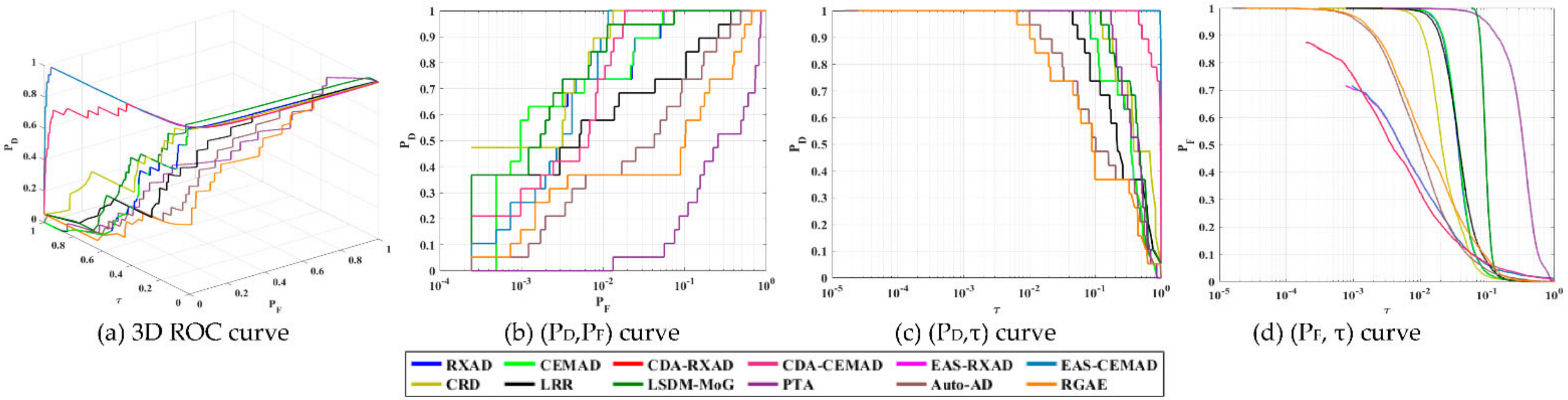
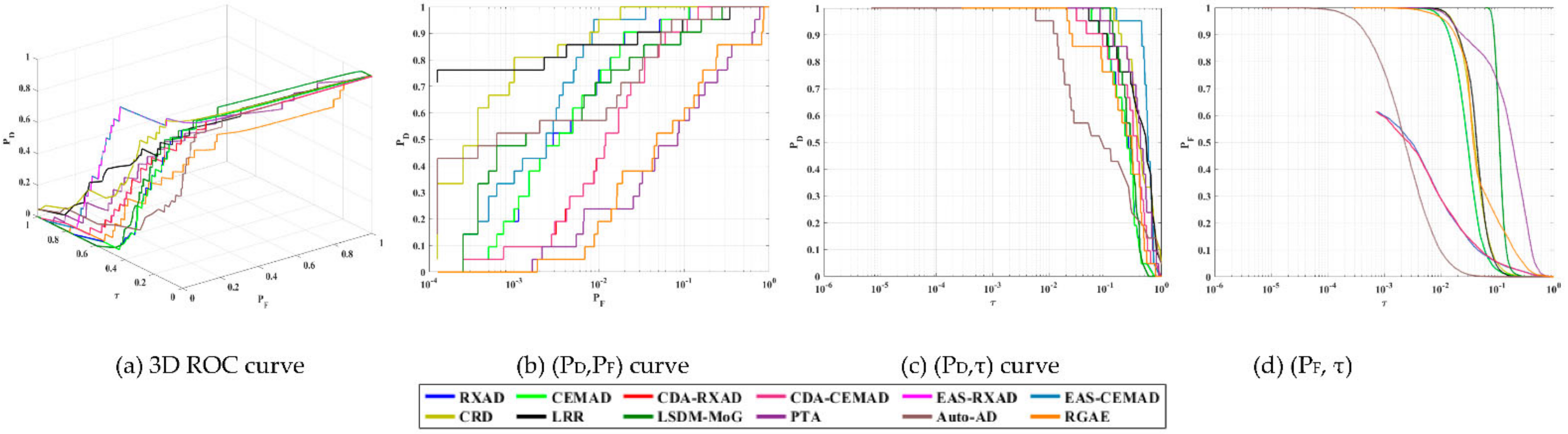
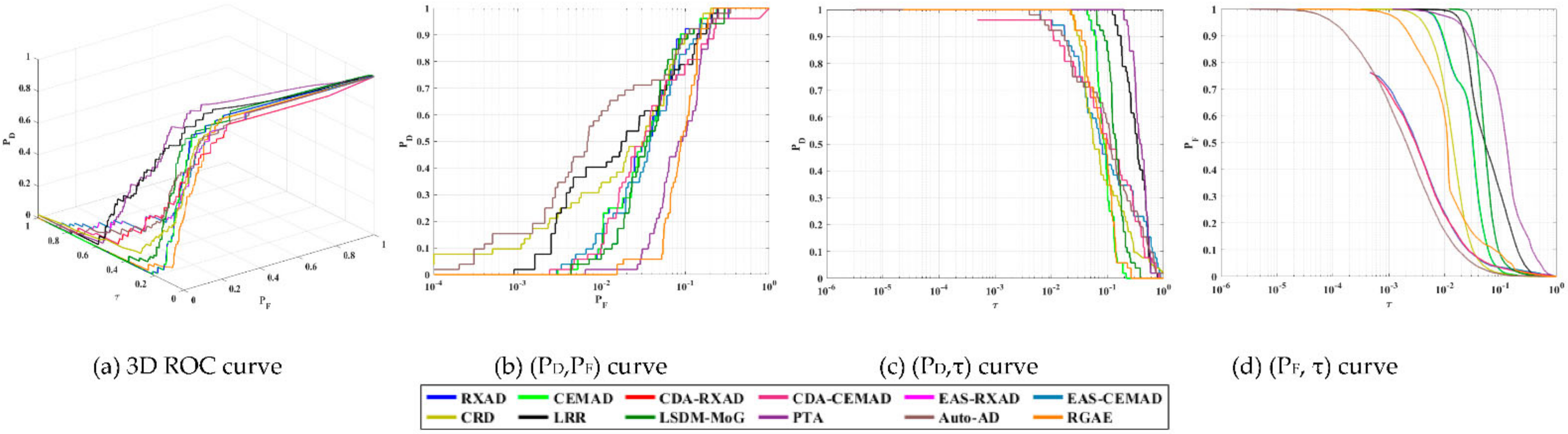
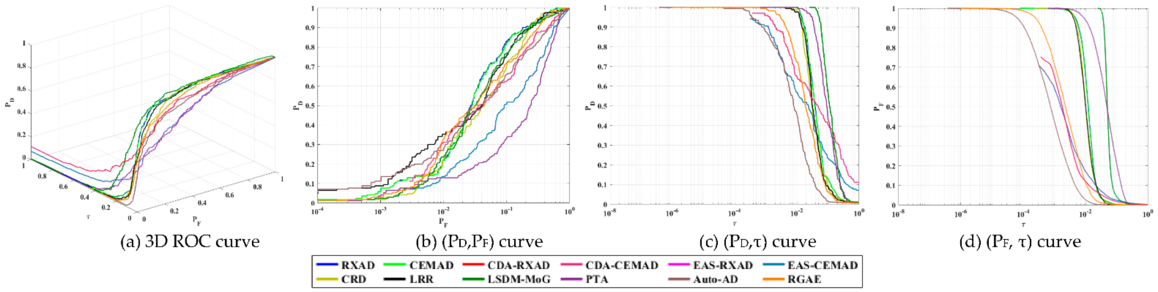
(D,F), which is very likely to lead to incorrect conclusions. In addition, there is a lack of criteria to measure anomaly detectability as well as BS. To address this issue, a 3D ROC analysis developed recently in [16,18] provide a feasible solution. It deviates from the traditional 2D ROC curve of (PD,PF) by considering the threshold value τ as an independent parameter to make both PD and PF dependent functions of τ. As a consequence, a 3D ROC curve becomes a plot of three parameters, PD, PF, τ, which can be used to generate three respective 2D ROC curves of (PD,PF), (PD,τ) and (PF,τ), each of which produced its own AUC values, AUC(D,F), AUC(D,τ) and AUC(F,τ). By manipulating these three AUC values, eight AD measures can be further derived to evaluate anomaly detectability, BS, joint anomaly detectability and BS from all around aspects for AD performance.
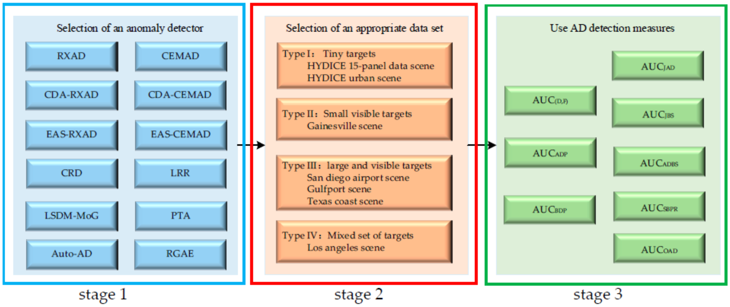
Finally, we come to the most crucial issue, which is how to select an appropriate dataset for AD. There are many datasets available on websites that can be used for AD. This paper particularly selects the seven most popular datasets for experiments and conducts a very comprehensive and comparative analysis. These datasets can be categorized into four types of data sets, Type I–Type IV. The two data sets of Type I consist of hyperspectral digital collection experiment (HYDICE) panel data scene and HYDICE urban data scene which contain tiny or barely recognizable targets as anomalies. A data set of Type II, the Gainesville scene, has relatively small visible targets that may only occupy a few full pixels and can be viewed as anomalies. Three data sets of Type III comprise of a San Diego Airport scene, Gulfport scene and Texas coast scene, each of which contains large and visible targets that are hardly considered to be anomalies. The data set of Type IV, a Los Angeles scene, is a mixed-data scene which contains targets of different sizes made up of a data set of Type II that contains small targets and a data set of Type IV that contains large targets. So, for data sets of Type I and II, the detector to be used should be an anomaly detector because the targets to be detected are small and nearly invisible. By contrast, the detectors used for the targets in data sets of Type III and IV should be considered target detectors rather than anomaly detectors because the targets are large and visible and the required target knowledge can be obtained directly by visual inspection. This type of knowledge obtained from observation, i.e., visual inspection, is generally referred to as a posteriori target knowledge. A target detection (TD) method using such a posteriori target knowledge is called a posteriori target detection (PSTD). Now, if we apply PSTD and AD to data sets of Type III and IV, their respective detection results are quite different, as are their drawn conclusions. The most troublesome issue resulting from using data sets of Type III and IV is that a true anomaly detector may not detect large targets as anomalies, but rather detects real anomalies at somewhere else which are not identified by the GT. Consequently, AD using this type of dataset may perform worse than PSTD, which performs TD using the obtained a posteriori target information. Another issue is that the GT maps provided by these datasets may only include targets which can be identified by visual inspection but may not include true anomalies, which cannot be identified through visual inspection or prior knowledge. Therefore, using a visual-based GT to evaluate an anomaly generally yields misleading conclusions, as will be shown later in the experiments.
To see the differences between PSTD and AD, this paper further explores the above issues and performs a detailed comparative analysis on AD and PSTD via extensive experiments. A comprehensive study, along with a detailed comparative analysis, was also conducted for TD and AD via 3D ROC curve-analysis. Specifically, data sets of Type II–Type IV were used for PSTD and AD to simply provide hard evidence that PSTD and AD can lead to different conclusions.
The major contributions of this paper are summarized as follows.
  • This paper is believed to be the first work to investigate the suitability issue of data scene characterization for AD. In particular, it categorizes data scenes into four types of dataset. It further shows that data sets of Type I and II are suitable for AD, while data sets of Type III and IV are not appropriate for AD or PSTD.
  • A comprehensive study and analysis on four different types of dataset was conducted for AD to illustrate and demonstrate that different conclusions can be drawn for various anomaly detectors from datasets of different types.
  • A comparative study and analysis was also performed on data sets of Type III and IV using PSTD and AD to reveal their quite different conclusions.
  • To evaluate the detection performance of various data scenes, the 3D ROC analysis provides creditable assessments for AD methods and data scenes in terms of BKG and noise issues.

2. Methods

As mentioned in the introduction, the first issue is to select an effective anomaly detector. This section reviews and discusses commonly used AD methods that will be used for experiments. They can be categorized into four categories, statistical AD (SAD), BKG-suppressed/removed based AD, low rank and sparse space decomposition-based AD and deep learning-based AD methods.

2.1. Statistical AD

SAD is well-studied and has been investigated extensively in the past. It is derived from the signal detection in noise model based on a binary hypothesis testing problem which is described by [17] as follows:
H 0 : r noise versus H 1 : r signal + noise
where hypotheses H0 and H1 are the “null hypothesis” which represents signal absence with noise and the “alternative hypothesis” which represents signal presence, each of which is governed by their probability distributions, p0(r) and p1(r). Assume that the prior probabilities of H0 and H1 are given by P(H0) and P(H1), respectively. Also, let cij be the cost incurred by a decision saying Hi when Hj is true. The optimal detector is derived as a Bayes detector δBayes(r) given by the following formula:
δ LRT ( r ) = 1 ,   if   Λ ( r ) τ 0 ,   if   Λ ( r ) < τ .
where Λ(r) = p0(r)/p1(r) is a likelihood ratio test (LRT) and the threshold τ is given by τ = ( c 10 c 00 ) P ( H 0 ) ( c 01 c 11 ) P ( H 1 ) . Using (2), the detection probability PD and false alarm probability PF can be calculated by the following equations:
P D = Λ ( r ) τ p 1 ( r ) d r
P F = Λ ( r ) τ p 0 ( r ) d r
Since the τ in (2) is determined by the prior cost cij and the prior knowledge of probabilities, P(H0) and P(H1), they are not generally available in practical applications. To resolve this issue, the Neyman–Pearson (NP) detection theory is widely used to replace τ with a constraint β imposed on PF in (4) and then to maximize the detection probability PD in (3), as follows:
max δ P D ( δ ( r ) )   subject   to   P F ( δ ( r ) ) β .
The resulting detector is called an NP detector, which is shown in [5] to be the same LRT as (2) given by the following formula:
δ NP ( r ) = 1 ,   if   Λ ( r ) > τ 1   with   probability   γ   if   Λ ( r ) = τ 0 ,   if   Λ ( r ) < τ
where the threshold τ and γ can be determined by solving the following formula:
P F ( δ ( r ) ) = Λ ( δ ( r ) ) > τ p 0 ( r ) d r + γ Λ ( δ ( r ) ) = τ p 0 ( r ) d r = P 0 ( Λ ( r ) > τ ) + γ P 0 ( Λ ( r ) = τ ) = β τ = P F 1 ( β )
The major advantage of using the NP detector (6) over (2) is that no prior knowledge of cij and P(H0), P(H1) is required. Instead, the NP detector is determined by its level of significance β which is specified by users. However, the probability distributions p0(r) and p1(r) are still required. Unfortunately, in many practical applications, these probability distributions are not available. In this case, the LRT in (2) must be replaced with a specific detector without appealing for p0(r) and p1(r). This leads to many detectors developed for different criteria in the literature [26].

2.1.1. Reed–Xiaoli AD

It should be noted that model (1) is specifically designed for TD where the signal to be detected along with p0(r) and p1(r) that govern the two hypotheses must be known a priori. Unfortunately, when (1) is applied to anomaly detection, there are two issues that needed to be addressed. One is the targets of interest which are unknown. The other is p0(r) and p1(r), which are also unknown. To resolve this dilemma, the well-known Reed–Xiaoli anomaly detector (RXAD) was developed in [4] to mitigate these issues. Its aim is to formulate an anomaly detection problem as a binary composite hypothesis testing problem to detect a target specified by a known target shape with an unknown amplitude α. (i.e, abundance). It assumes that there is reference data (or secondary data) governed by Gaussian distributions which can be used to estimate the parameter α. The resulting detector is called the generalized likelihood ratio test (GLRT) [27,28,29]. However, from a practical viewpoint, these assumptions may not be realistic.
Furthermore, many researchers who are working on AD have taken RXAD for granted without bothering how it is derived. As a matter of fact, it is believed that people who know how to implement RXAD as Mahalanobis distance but did not know why. Specifically, many of them may even have difficulty with fully understanding mathematical derivations given in [27,28,29]. To offer an alternative to approaches derived in [27,28,29], in what follows, we describe an approach proposed in [3] which took a rather simple perspective to arrive at the same RXAD derived in [27,28,29].
It models an anomaly detection problem as a subpixel detection problem by extending the binary simple hypothesis testing problem in (1) to the following binary composite hypothesis testing problem:
H 0 :   r = n versus H 1 :   r = α t + n
where r is a data vector and n is a noise vector characterized by a Gaussian distribution with the mean μn and covariance matrix K. Specially, in (8), αt is a subpixel target where t is specified by a priori target spectral signature vector and α is an unknown target intensity parameter such as abundance fraction of t, which is assumed to be unknown and needs to be estimated. Since the parameter α needs to be estimated before (8) is carried out for TD specified by (1), (8) is quite different from (1). In this case, we can construct p 0 ( r ) ~ N ( μ n , K ) and p α ( r ) ~ N ( α t + μ n , K ) are two Gaussian distributions under H0 with the mean μ n and H1 with the mean α t + μ n respectively. The solution to (8) is called GLRT given using the following equation:
δ GLRT ( r ) = Λ ( r ) = max α p α ( r ) p 0 ( r ) = exp r α ^ MLE ( r ) t μ n T K 1 r α ^ MLE ( r ) t μ n exp r μ n T K 1 r μ n log Λ ( r ) = 2 α ^ MLE ( r ) t K 1 r μ n
where
α ^ MLE ( r ) = arg max α p α ( r ) = arg min α r α t μ n T K 1 r α t μ n
is the maximum likelihood estimation (MLE) is used to estimate α. The solution to (10) can be found as follows.
Differentiating r α t μ n T K 1 r α t μ n in (5) with respect to α and letting it be zero, i.e.,
r α t μ n T K 1 r α t μ n α α ^ MLE ( r ) = 0 2 t T K 1 ( r μ n ) + 2 α ^ MLE ( r ) t T K 1 t = 0
which results in
t T K 1 ( r μ n ) = α ^ MLE ( r ) t T K 1 t α ^ MLE ( r ) = t T K 1 ( r μ n ) t T K 1 t = ( r μ n ) T K 1 t t T K 1 t .
Substituting (12) into (9) yields
δ GLRT ( r ) = 1 ;   if   t T K 1 r μ n 2 t T K 1 t τ 0 ;   if   t T K 1 r μ n 2 t T K 1 t < τ
with τ = ( 1 / 2 ) log τ .
The GLRT in (13) is also called an adaptive matched filter (AMF) in [30] along with its square root also being known as a matched filter (MF) [31]. However, in (8) and (13), the target of interest, t is assumed to be known for TD. But practically, it should be unknown in AD. Therefore, (13) cannot be directly used for AD. In order to cope with this problem, we introduce the dummy variable trick (DVT) proposed by Chang [32] which is defined as follows.

Dummy Variable Trick (DVT)

For problem A, which cannot be solved directly, the dummy variable trick (DVT) introduces an auxiliary variable ξ to reformulate problem B which is solvable where ξ is used as a liaison to bridge problem A and problem B and will be vanished after the problem is solved by B. Because of its functionality, ξ is considered a dummy variable.
Because AD does not have any prior knowledge of targets that it is looking for, (13) is not applicable to AD. Interestingly, the DVT plays a liaison role between TD and AD. Specifically, we can replace the known target t in (13) with an unknown specified target (UST), t UST to derive a t UST -specified GLRT, δ t UST GLRT ( r ) defined by
δ t UST GLRT ( r ) = 1 ;   if   t UST T K 1 r μ n 2 t UST T K 1 t UST τ 0 ;   if   t UST T K 1 r μ n 2 t UST T K 1 t UST < τ
which becomes a function of two dual variables, the data sample vector r and the unknown specified target t UST . Due to the fact that AD does not have any prior target knowledge, AD intends to find data samples that yield the maximum values of δ t UST GLRT ( r ) over all possible t UST for any given data sample vector r. This allows us to reformulate (14) as the following optimization problem
t * = arg max t UST δ t UST GLRT ( r )
with the optimal solution t * solved by Schwarz’s inequality and given by
t * = κ r μ n   subject   to   any   constant   κ .
substituting (16) into (14) yields a t * -specified GLRT,
δ t * , κ GLRT ( r ) = κ r μ n T K 1 r μ n .
by setting κ = 1 in (17), δ t * , κ = 1 GLRT ( r ) turns out to exactly δ RXAD ( r ) in [3,26] given by
δ t * , κ = 1 GLRT ( r ) = δ RXAD ( r ) = r μ n T K 1 r μ n
which is also known as Mahalanobis distance. More details of theoretical derivations of RXAD can be found in [3].

2.1.2. CEMAD

In [33], Chang and Chiang developed an alternative approach to RXAD, called R-AD, which replaces K with the global sample auto-correlation matrix R given by
δ R - AD ( r ) = r R 1 r
which has been shown to perform comparably to RXAD in [4]. One advantage of R-AD over RXAD is that R-AD does not need to calculate the mean μ n . So, for real-time AD, R-AD is more appropriate than RXAD because R can be directly calculated by Woodburry’s identity in real time ([34] Appendix A). However, its theoretical support was not provided until recently when R-AD was re-derived as a constrained energy minimization anomaly detector (CEMAD) in [32].
Instead of using GLRT, CEMAD designs a detector δ(r) which also assumes a signal embedded in an additive noise specified by the alternative hypothesis in (1). However, instead of using costs, {cij} and prior probabilities of hypotheses, P(H0) and P(H1) as the Bayes detector in (2) does, it uses a criterion, called deflection, D(δ(r)) defined in [35] using the following formula:
D ( δ ( r ) ) = E [ δ ( r ) | H 1 ] E [ δ ( r ) | H 0 ] 2 var [ δ ( r ) | H 0 ]
where E [ δ ( r ) | H j ] is an expectation calculated using the probability density function pj(r) under hypothesis Hj. Equation (20) turns out to be the signal-to-noise ratio (SNR) derived by the Bayes detector in (2). It should be noted that (20) also assumes the prior knowledge of the signal in (1) which can be considered to be specified by a particular target of interest, t and its SNR is also determined by t specified in H1. The rationale for using SNR can be found in the bottom paragraph ([17], eq. II.B.31). In fact, SNR is the parameter that determines false alarm PF and detection probability, PD is referred to in more detail in ([17], (III.B.33), p. 56).
By virtue of (20), we can use SNR to derive an alternative theory to LRT, called SNR detection theory, which designs detectors without appealing for probability density functions, p0(r) and p1(r) used in LRT and GLRT. More specifically, (20) can be re-expressed in terms of SNR as follows:
D ( δ t ( r ) ) = SNR ( δ t ( r ) )
where t is included to emphasize the dependency of SNR on t. However, (21) is still determined by the unknown t and cannot be directly applied to AD. Adopting a similar approach to the derivation of t UST -specified GLRT, δ t UST GLRT ( r ) in (14) using DVT allow us to define t UST -specified SNR, SNR ( δ t UST ( r ) ) by replacing t with t UST as follows.
D ( δ t UST ( r ) ) = SNR ( δ t UST ( r ) ) .
Furthermore, we use the SNR in (22) as a criterion for optimality to design a finite impulse response (FIR) filter specified by
δ w ( r ) = w T r
via a weighting vector w where the detector δw operating on the original data space X with r X . Coincidentally, this approach is similar to that used to derive CEM in [36] which utilizes minimum variance (i.e., least squares error) rather than SNR as an optimal criterion. Like GLRT, CEM also assumes prior knowledge of the desired target d. So, a direct use of CEM for AD is not applicable. To resolve this issue, we follow an approach developed in [32] to derive CEMAD.
Suppose that a hyperspectral image is represented by a collection of image pixel vectors, denoted by r n n = 1 N with r n = r n 1 , r n 2 , , r n L T being an L-dimensional pixel vector and L being the total number of spectral bands. Rewriting (23) by replacing r with rn yields
δ ( r n ) = w T r n .
The averaged output energy of (24) over the entire image scene can be obtained by
1 N n = 1 N δ 2 ( r n ) = w T R w
where R = 1 N n = 1 N r n r n T is the sample autocorrelation matrix, N is the total number of data sample vectors and L is the number of spectral bands. Then, CEM is designed to find the solution to the following constrained optimization problem,
min w w T R w   subject   to   d T w = 1 .
which is given using the following formula:
δ d CEM ( r ) = w CEM T r = d T R 1 r d T R 1 d
where the subscript “d” is included to emphasize the use of the desired target d. The minimum variance resulting from (27) can be obtained using the following formula:
w CEM T R w CEM = d T R 1 d 1
And its SNR is given by the following formula:
SNR δ d CEM ( r ) = d T R 1 d T
Interestingly, by means of DVT, we can use t UST to replace d in (26) as the constraint t UST T w = 1 to derive a t UST -specified CEM given using the following formula:
δ t UST UST - CEM ( r ) = t UST T R 1 r t UST T R 1 t UST .
Since we do not know that t UST and t UST T R 1 t UST 1 are constants, it does not make sense that include this unknown constant in the detector design. In this case, we can replace the constraint t UST T w = 1 with the SNR constraint, i.e., SNR δ t UST UST - CEM ( r ) = t UST T R 1 t UST to replace d T w = 1 used in (26). The resulting constrained optimization problem is then given by the following formula:
min w w T R w   subject   to   t UST T w = SNR δ t UST UST - CEM ( r ) = t UST T R 1 t UST .
The solution to (31) is called t UST -specified SNR-based CEM, δ t UST SNR - CEM ( r ) , which was derived in [32] by the following formula:
δ t UST SNR - CEM ( r ) = t UST T R 1 r .
where the denominator t UST T R 1 t UST in (30) disappears in (32). As noted, in order for δ t UST SNR - CEM ( r ) to perform AD, the desired CEM anomaly detector (CEMAD), δ κ CEM - AD ( r ) must be the one that finds the maximum SNR, as follows:
δ κ CEM - AD ( r ) = arg max t UST δ t UST SNR - CEM ( r ) = κ r T R 1 r
where κ is any constant. By letting κ = 1 , δ κ = 1 CEM - AD ( r ) is reduced to RAD in (19).
More details of theoretical derivations of CEMAD can be found in [32].

2.1.3. RXAD/CEMAD Variants

According to (18) and (19), RXAD and CEMAD involve two processes in sequence. One is to first invert the global sample covariance matrix K by RXAD in (18) or the global sample correlation matrix R used by CEMAD in (19) to suppress the global background (BKG). It then uses a matched filter with r μ n as the matched signal by RXAD in (18) or the data sample r as the matched signal used by CEMAD in (19) to extract data samples that match the matched signal. However, a target that is considered an anomaly has distinct spectral compared to the spectral characteristics of its surrounding data samples. So, for an anomaly detector to be effective, spectral correlation among neighborhood pixels has a crucial role in identifying an anomaly. In doing so, many RXAD/CEMAD-type detectors and variants have been developed along this line in the past. Examples include local RXAD [37,38], support vector data description (SVDD) by Banerjee et al. [39], weighted-RXAD and linear filter-based RXAD by Guo et al. in [40], a sliding window by Chang et al. [41], a dual window-based eigen separation transform (DWEST) by Kwon et al. [42], followed by CRD which also used dual windows in [43], and multiple-window-anomaly-detection (MWAD) by Liu and Chang on [44] by making use of multiple windows to perform AD adaptively, guided filtering-based AD by Tang et al. in [45], spectral-spatial feature extraction-based AD by Lei et al. [46], a nonlinear anomaly detector, kernel-based RXAD by Wang et al. in [47] and,, most recently, an iterative spectral-spatial hyperspectral anomaly detector (ISSHAD) by Chang et al. [5]. In addition, there were also AD methods developed for various applications, such as unlabeled classification by Wang et al. [48], real time processing of anomaly detection by Chen et al. [49]. Recently, Liu et al. [50] extended AD by considering the Gaussian background with an unknown covariance matrix from which two equivalent adaptive GLRT-based detectors. Yuan et al. [51] proposed an AD method by constructing a vertex- and edge-weighted graph to detect anomalies with better accurate detection performance and better robustness to noise where no background distributions are required. Kang et al. [52] developed an attribute and edge-preserving filtering-based detection method (AED) by fusing the multiscale information extracted by attribute and edge-preserving filters.

2.2. Background-Suppressed/Removed AD

No matter how well RXAD/CEMAD can be improved by different modifications, these RXAD/CEMAD-variants still suffer from a severe issue, anomalies embedded in the BKG which cannot be separated from the BKG. To address this issue, many recent approaches have been directed to how the BKG can be effectively suppressed/removed to improve the detectability of an anomaly detector including RXAD/CEMAD. The key idea is to follow exactly the throw-before-detection strategy proposed in [3], which attempts to throw away BKG prior to AD. Two approaches are of particular interest, BKG estimation/reconstruction and BKG separation.

2.2.1. BKG Estimation

BKG estimation is generally based on an assumption that the BKG can be characterized and modeled by Gaussian distributions. For example, in [53] Qu et al. developed a Gaussian mixture model (GMM)-based approach to anomaly extraction and an effective GMM-based weighting approach for fusing the extracted anomaly maps which can be further rectified by using a guided filter to obtain the final anomaly detection map. On the other hand, BKG reconstruction is generally done by deep learning (DL)-based methods which use training samples to tune the parameters that specify the used models [54], autoencoder (AE) [55,56,57], generative adversarial network (GAN) [13,15,58] and robust graph autoencoder (RGAE) [59]. All these methods are based on an assumption that the estimation/reconstruction error is the main cause incurred by anomalies.

2.2.2. BKG Decomposition for Separation-Based AD Methods

BKG estimation/reconstruction is not the only way to improve BS. Chang et al. in [60] developed a BKG anomaly component projection and separation optimized filter (BASO) to separate anomalies from the BKG. In a recent work, Li et al. in [22] also took advantage of tensor decomposition to develop a prior-based tensor approximation (PTA) which decomposed a hyperspectral imagery into a background tensor and an anomaly tensor corresponding to the BKG and anomaly spaces, respectively, for hyperspectral anomaly detection so that the anomalies can be detected in the anomaly tensor.

2.3. Low Rank and Sparse Subspace Decomposition-Based AD

In Section 2.1, SAD takes care of spectral neighborhood information of anomalies via manipulating local windows or using adaptive weights of data samples surrounding anomalies. However, there is another way to deal with this issue. Based on the assumption that anomalies are embedded in the BKG, recent studies have been devoted to decomposing the data space X into two disjointed subspaces, a low rank subspace and a sparse subspace which correspond to the BKG space and anomaly space, respectively.

2.3.1. Low Rank and Sparse Representation

An early approach to subspace decomposition is low rank representation (LRR) which formulates AD as the following basic optimization problem [6].
min S , E rank ( S ) + λ | | E | | 2 , 1   subject   to   X = D S + E
where D is the BKG dictionary with S being representation coefficients and E is its residual, and | | | | 2 , 1 is the l2,1 norm defined as the sum of l2 norm of the column of a matrix. The parameter λ is used to regularize the sparse representation E. In other words, DS and E represent the BKG and anomalies, respectively. The idea of LRR is to find the BKG dictionary D and constrains sparse subspace S so as to produce an anomaly subspace. Many works based on (34) have been reported.

2.3.2. Low Rank and Sparse Subspace Decomposition-Based AD

Unlike LRR which uses (34) to create a BKG dictionary while regularizing the sparse representation, a more attractive approach is to decompose the BKG and anomalies into two separate subspaces to be discussed in the following.

2.3.3. Low Rank and Sparse Subspace Decomposition

An earlier approach to subspace decomposition is robust principal component analysis (RPCA), developed by Candes et al. [19], which is a blind source separation technique to decompose the data matrix X into
X = L + S
In a matrix decomposition, similarly, analogous to RPCA, an approach developed by Vaswani et al. [20,21], called robust subspace learning (RSL), treats outliers as additive sparse corruptions via sparse + low-rank (S + LR) matrix decomposition. With this interpretation, RPCA can be considered a variant of RSL via S + LR formulation. Li et al. modified (34) in [61] to become a low-rank and sparse decomposition model with a mixture of Gaussians (LSDM-MoG) where the sparse component can be described by a mixture of Gaussian noises so that anomalies can be detected by the Manhattan distance. However, (35) only offers the separation of these two spaces with anomalies sandwiched between the BKG and noise. That is, RPCA and RSL via S + LR do not distinguish anomalies from the noise or outliers in separate component spaces.

2.3.4. Low Rank, Sparse Noise Subspace Decomposition

A recently developed approach which extended (35) to include noise as a separate component is low-rank and sparse matrix decomposition (LRaSMD) proposed by Zhou and Tao [7] who developed go decomposition (GoDec) to decompose the data space X into a low rank subspace L and a sparse subspace S as
X = L + S + N
with the noise N separated in a third component space. In order to better detect anomalies, GoDec did not use the commonly used parameters to regularize the sparse representation S such as model (34) used by LRR [6]. Instead, it introduced the concept of sparsity cardinality (SC) to find an SC-constrained anomaly space from which anomalies can be extracted. This unique property was not found in any low-rank and sparse representation-based approach. Interestingly, it is also this SC that makes LRaSMD very competitive. Unfortunately, GoDec in [7] did not discuss how SC it works and how SC was determined. In [62] Zhang et al. took advantage of the LRaSMD model using the Mahalanobis distance as an anomaly detection method.
Most recently, a component decomposition analysis (CDA) was further developed by Chen et al. [12] to actually extend RPCA and RSL via S + LR to a three-component model which decomposes principal components (PCs), independent components (ICs) and noise component into three separate component spaces as
X = P C s + I C s + N .

2.4. Effective Anomaly Space

It is known that anomalies are sandwiched between the BKG and noise [10]. On one end, anomalies can be embedded in the BKG. To another end, anomalies can be mistakenly treated as noise. Despite the fact that the LRaSMD model (36) decomposes X into a (L,S,N)-component space, two issues still remain. One is how to determine the model order for each subspace. Another is how to take care of non-Gaussian noise. To address this issue, a notion of effective anomaly space (EAS) was coined in [10] and developed to meet this need. It proposed a sandwich model which considers anomalies to be sandwiched between the BKG and noise, and then separates anomalies from both the BKG and noise so that anomalies can be detected in EAS more effectively. More specifically, EAS is a space which is particularly constructed for an arbitrary anomaly detector to suppress the BKG via data sphering (DS) as well as to remove noise jointly and simultaneously so as to improve anomaly detectability. The inclusion of DS in EAS was derived from an approach developed by Chang and Chen in [63] which used DS to remove the first-order and second-order data statistics to produce sphered data, X DS . The idea of DS is not new and has been widely used in communications and signal processing [11]. It maps the original data sample vector r to its sphered data sample vector r ^ in the sphered data space X ^ by r ^ = K 1 / 2 r μ where K 1 / 2 is referred to as whitening matrix, μ and K are global mean and global sample covariance matrix. Details of DS can be found in ([64] Section 6.3.1) along with its code [64] (pp. 1000–1001). The DS process has been shown to be more effective than many approaches which use Gaussian-based models, such as the MoG proposed in [53,61] that can be completely annihilated by X DS before MoG leaks into the sparse space, low rank representation that is characterized by 2nd order statistics.

2.4.1. Estimation p

To construct EAS, the first task is to estimate the order of the low rank space L, m, and the order of the sparse space S, j, respectively. Instead of directly estimating m, EAS takes advantage of the concept of virtual dimensionality (VD) [1,65,66,67] which is defined as the number of spectrally distinct signatures, p, present in a hyperspectral image. If we further assume that m and j can be used to specify the number of BKG signatures and sparse signal sources, respectively, then p = m + j . In other words, m can be estimated by VD via m = p j . Since VD has been widely used in hyperspectral imaging and its code is available in [64] (pp. 997–1000).
Although DS can remove noise characterized by second-order statistics including Gaussian noise and Gaussian BKG from the original data space X, non-Gaussian noise still exists in X DS . EAS adopts a rather different approach by taking advantage of the blind source separability resulting from ICA [11] to extract anomalies from independent components (ICs). Unfortunately, such ICA-generated ICs cannot separate non-Gaussian noises from anomalies since non-Gaussian noises are also characterized by high order-statistics and likely mixed with anomalies in ICs. EAS resolves this issue by using VD to estimate the total number of spectrally distinct target signal sources and minimax singular value decomposition (MX-SVD) [68] to estimate a desired number of prioritized ICs, j, needed to form an IC subspace, X I C j which can also be considered to be anomaly space, X AS . In order to further clean up the leakage form non-Gaussian noises into I C j , the idea of sparsity cardinality (SC) proposed in [7] is then used for non-Gaussian noise removal due to the fact that noise cannot be sparse and can be eliminated by SC. Including SC into I C j yields EAS, X EAS = X SC I C j . For detailed implementations we refer to [10].

2.4.2. MX-SVD Estimating j

Once p is found by VD, the follow-up issue is to estimate j so that m can be therefore determined by m = p j . Since anomalous signal sources can be considered rare signal sources, MX-SVD developed in [68] originally developed to estimate the rank of rare signal space can be used for this purpose.

2.4.3. Construction of Effective Anomaly Space

After m and j are estimated by VD and MX-SVD, an anomaly space, X AS , can be obtained by X I C j , i.e., X AS = X I C i . Although X DS already removes Gaussian noise via DS, X AS may still contain non-Gaussian noises. To further resolve this issue, the concept of SC developed in [10] is imposed on X AS to construct X EAS = X SC I C j . This is because noise cannot be sparse and SC allows X AS to retain only the first k largest nonzero samples in X AS by setting the rest of data samples to zeros where k can be obtained by setting SC = k = j × N according to [64]. Details of exploring the SC concept can be found in [10]. A software tool developed for constricting EAS is available on the following website: https://wiki.umbc.edu/download/attachments/26281078/EAS%20by%20Chein-I%20Chang.zip?api=v2 (accessed on 22 December 2023).

3. Materials and Experiments

For a selected AD method such as those discussed in Section 2, two issues have significant impacts on AD performance. One is the selection of an appropriate evaluation tool that measures the effectiveness of an anomaly detector in various aspects not only limited to anomaly detectability. The other is the selection of a proper dataset to illustrate the efficacy of an anomaly detector. Interestingly, these two issues have been overlooked in the past. Many works on AD reported in the literature have followed the traditional approach which uses the classic 2D ROC analysis as an evaluation metric for AD and popular available datasets for experiments without justifying the goodness of their proposed AD methods. For example, the area under the ROC curve of (PD,PF), AUC(D,F) is originally developed as a criterion to evaluate TD in noise from the Neyman–Pearson theory but not designed for AD for BS. As a second issue, several commonly used datasets, such as San Diego Airport, Gulfport, Texas coast and Los Angeles data scenes have been widely used to evaluate anomaly detectors for AD performance; however, the targets in these scenes are large and visible airplanes, which can be hardly considered anomalous targets. So, if we assumed these airplanes to be real anomalies, then the conclusions drawn from this assumption would have had been misleading. Two attributes have contributed to this problem. One is how GT is collected. Is it collected by prior knowledge or visual inspection? To the authors’ best knowledge, this has never been investigated. A second issue is that the provided GT does not include real anomalies but rather large targets as anomalies like San Diego Airport and Gulf data scenes. Although this issue was discussed in [10] a detailed study on this issue is yet to be investigated. This section takes up the above-mentioned issues and conducts a comprehensive study via extensive experiments on several popular datasets to demonstrate how important the selection of evaluation measures and datasets for AD is.

3.1. 3D ROC Analysis Theory for AD

The first issue to be discussed is how to select an effective performance metric to evaluate an anomaly detector. The signal detection model (1) is mainly used for known TD because H0 represents the case of noise in communications and signal processing. As pointed out in Section 2.4 BS is one of main key factors to have significant impact on AD. Therefore, (1) is no longer applicable to AD. To address this issue, we reformulate (1) as an anomaly detection model, as described in [18], as follows:
H 0 : r BKG v e r s u s H 1 : r anomlay + BKG
in which represents a two-class binary classification problem is represented by BKG and the anomalies are specified by two distinct classes. By virtue of (38), the detection of the BKG is as important as the detection of anomalies. Therefore, since PD is specifically described by anomaly detection probability (ADP), PADP, and the PF used for false alarm probability in (1) can now be changed to 1-PF used for BKG detection probability (BDP) in (38).

3.1.1. 3D ROC Curve Versus 2D ROC Curve

An effective evaluation tool for (38) is commonly known as 2D ROC curve which is a plot of (PD,PF) over the unit interval [0, 1]. However, there are also several issues of using such 2D ROC curves for analysis. The first and foremost is that both PD and PF are calculated by the same threshold τ. As a result, (PD,τ) and (PF,τ) cannot work independently. As a matter of fact, PD and PF interact with each other through τ and are actually dependent functions of an implicit independent parameter specified by τ. This issue brings up a second issue, which is that the area under curve (AUC) of (PD,PF), AUC(D,F), does not necessarily represent the target detectability of a detector. This is because a higher value of AUC(D,F)) indicates a higher value of PD, as well a higher value of PF. So, when the value of PF changes, so does the value of PD. A third issue is that on some occasions two detectors may yield different ROC curves, but they indeed produce the same value of AUC(D,F). Under this circumstance, both detectors have shown the same effectiveness in detection performance, but their anomaly detectability and BKG suppressibility may be quite different. This issue can only be addressed by calculating PD or PF independently, even their AUC(D,F)’s are the same. In other words, AUC(D,F) can only be used to evaluate the effectiveness of a detector but cannot evaluate its individual PD or PF. Last but not least, the 2D ROC curve lacks the ability to addressing the background (BKG) issue.
In order to resolve the above issues arising when using a 2D ROC curve, a 3D ROC analysis was first envisioned and applied to hyperspectral subpixel detection [16] where a 3D ROC curve was introduced as a function of three parameters, PD, PF and the threshold parameter τ. Its idea includes τ as an independent variable to produce PD, PF as its dependent values and then generates an ROC curve in a three-dimensional space of (PD,PF,τ). The resulting ROC curve is known as the 3D ROC curve. By virtue of such a 3D ROC curve three 2D ROC curves can be also generated, known as the 2D ROC curve of (PD,PF), 2D ROC curve of (PD,τ) and 2D ROC curve of (PF,τ) by projecting a 3D ROC curve on their own respective planes separately. The AUC values calculated from these three 2D ROC curves of (PD,PF), (PD,τ) and (PF,τ), referred to as AUC(D,F), AUC(D,τ) and AUC(F,τ) that can be further combined to derive eight different detection measures used to evaluate the performance of a detector from all round aspects described in detail as follows.

3.1.2. 3D ROC Curve-Derived Detection Measures

With this interpretation, the 3D ROC analysis-based evaluation tool developed for TD in [16] can be modified for AD in [18] to determine whether a data sample is BKG or anomalous target pixel. Using such a 3D ROC curve plotted by a function of the three parameters, PD, PF, τ, three 2D ROC curves of (PD,PF), (PD,τ), (PF,τ) can be generated along with their respective AUC values, AUC(D,F), AUC(D,τ), AUC(F,τ), to define the following AD measures.
(i)
Effectiveness of a detector.
0 AUC ( D , F ) 1
This is the most widely used criterion in signal detection. According to (39), it was specifically designed to evaluate the effectiveness of an anomaly detector but not AD and BS individually because PD and PF work jointly using the same threshold value τ but cannot work alone independently.
(ii)
Anomaly detection probability (ADP). Using AUC(D,τ), we define ADP using the following formula to evaluate anomaly detectability.
0 AUC ADP AUC ( D , τ ) 1
That is, the higher is the value of AUCADP, the better is the anomaly detector.
(iii)
The joint target detectability (JAD) of a detector. Using AUC(D,F) and AUCADP, we can further define a measure, the JAD, for a detector as AUCJAD with the following formula:
0 AUC JAD = AUC ( D , F ) + AUC ADP 2 .
In TD, PF is the false alarm probability and 1-PF is detection of noise. So, using 1-PF to evaluate the noise detection performance does not make sense for TD. However, this is not true for the binary hypothesis formulation for AD specified by (38), PF represents the probability of the BKG data samples falsely detected as anomalies. With this interpretation, 1-PF can be considered to be the probability of correctly detecting BKG samples.
(iv)
As for BKG detection probability (BDP), using AUC(F,τ) we can define BDP, AUCBDP, as a counterpart of ADP in (40) as follows:
0 AUC BDP = 1 - AUC ( F , τ ) 1 .
(v)
Joint BS (JBS). By combining AUC(D,F) and AUCBDP we can further define JBS as follows:
0 AUC JBS = AUC ( D , F ) + AUC BDP 2 .
(vi)
Joint anomaly detectability and BKG suppressibility (ADBS). In order to factor AUC(F,τ) into AUC(D,τ) we consider AD and BS working separately with different values of the threshold τ as an independent parameter. Since PF is caused by the probability of mis-detecting the BKG as an anomaly, this error probability should be subtracted from PD. To take care of this effect, AUCADBS is defined as
1 AUC ADBS = AUC ( D , τ ) - AUC ( F , τ ) 1 .
(vii)
Concerning overall anomaly detection (OAD), a second ADBS measure is derived from a classification point of view. It is defined by the following equation:
0 AUC OAD = AUC ADP + AUC BDP 2
where AUCADP is in (40) and AUCBDP is in (42).
(viii)
Signal-to-BKG Probability ratio (SBPR) is the last but most effective detection measure comes from a similar idea that is widely used in communications/signal processing, signal-to-noise ratio (SNR). The signal-to-BKG probability ratio (SBPR) is defined by the following equation:
0 AUC SBPR = AUC ADP AUC BDP
where AUCADP and AUCBDP are defined in (40) and (42), respectively. It is interesting to note that what the 3D ROC analysis is to TD in [16] has an equivalent role to what the 3D ROC analysis to AD in [18].
To facilitate the use of 2D/3D ROC analysis, MATLAB-based software codes developed for calculating AUC and plotting ROC are made available at the website of the Remote Sensing Signal and Image Processing Laboratory (RSSIPL), University of Maryland, Baltimore County (UMBC), https://wiki.umbc.edu/display/rssipl/10.+Download (accessed on 22 December 2023).

3.2. Materials

As for a second issue, how to select an appropriate dataset to be used for performance evaluation is also crucial. Despite the fact that many datasets have been used for AD, to the authors’ best knowledge, no work has been reported to discuss the appropriateness of the used datasets. This section is specifically devoted to addressing this issue where we specifically selected seven most popular datasets used in the literature for experiments. In particular, these datasets can be categorized into four types of datasets. A data set of Type I contains tiny targets as anomalies which are barely visible by visual inspection or appear to be invisible at subpixel scale. A data set of Type II contains small targets that are visible by visual inspection as anomalies. In this case, an anomaly may occupy only a few full pixels. A data set of Type III contains large and visible targets which occupy a large number of full pixels; so, according to a general understanding, the targets in datasets of this type cannot be considered to be anomalies, but rather targets which can be obtained directly from the data to be used by visual inspection. A data set of Type IV contains a mixed set of targets of different sizes including small and large visible targets as anomalies. Using datasets of this type, we can evaluate how an anomaly detector performs when both small and large targets are present in the data. As will be shown in the following experiments, various anomaly detectors yield different conclusions.

3.2.1. Data Sets of Type I

HYDICE 15-Panel Data Scene

The first dataset is the HYDICE scene shown in Figure 1, which was collected in August 1995 from a flight altitude of 10,000 ft with the ground sampling distance approximately 1.56 m. This scene has been studied extensively by many reports such as [1,2,3]. A total of 169 bands were used for the experiments with low signal/high noise bands: bands 1–3 and bands 202–210; and water vapor absorption bands: bands 101–112 and bands 137–153 removed. There are 15 square panels in Figure 1a with three different sizes, 3 m × 3 m , 2 m × 2 m and 1 m × 1 m respectively. Due to the ground sampling distance of approximately 1.56 m, each of panels in the 1st column except the 1st row contains two panel pixels highlighted by red, p211, p221 in row 2, p311, p312 in row 3, p411, p412 in row 4, p511, p521 in row 5 as shown in Figure 1. All of the remaining 11 panels in Figure 1 contain one single panel pixel for each panel also highlighted in red, p11, p12, p13 in row 1, p22, p23 in row 2, p32, p33 in row 3, p42, p43 in row 4, p52, p53 in row 5. Therefore, there are a total of 19 red panel pixels. Figure 1b shows their precise spatial locations with the pixels in yellow indicating panel pixels mixed with the BKG.

HYDICE Urban Scene

A second HYDICE data scene, shown in Figure 2a, is an urban scene and comprised 210 spectral bands with 174 bands being used for experiments after the noise and water absorption bands had been removed. A region with a size of 80 × 100 pixels located at the upper right of the scene was selected as the test image shown in Figure 2b along with the GT map shown in Figure 2c where twenty-one pixels were identified as anomalies, which were cars and roofs because they had spectra that differ from the BKG.

3.2.2. Data Sets of Type II

The Gainesville dataset is an urban scene shown in Figure 3a. It was collected by an AVIRIS sensor over Gainesville, FL, USA. Removing the water absorption and low signal-to-noise ratio (SNR) bands from the original data yields 191 bands for experiments. The spatial resolution and size of this dataset are 3.5 m/pixels and 100 × 100 pixels, respectively. As shown in Figure 3a, this dataset contains relatively small targets as shown in the GT map in Figure 3b. A total of 52 anomalous pixels account for 0.52% of the image pixels to be explored for experiments.

3.2.3. Data Sets of Type III

San Diego Airport Scene

A third type of dataset used for experiments was also an airborne visible/infrared imaging spectrometer (AVIRIS) acquired scene, which is a San Diego airport scene in CA, USA with pseudo-color shown in Figure 4a. It has a size of 400 × 400 pixels with a 3.5 m spatial resolution and 224 spectral channels in wavelengths ranging from 370 to 2510 nm. After removing the bands that correspond to the water absorption regions, low signal-to-noise ratio and bad bands (1–6, 33–35, 97, 107–113, 153–166 and 221–224). In total, 189 available bands of the data were retained in the experiments. An area of 100 × 100 pixels at the upper left corner of the scene was selected as the test image shown in Figure 4b along with its GT map shown in Figure 4c. It is an urban scene in which the main BKG materials are rooves, shadows, and grass. There are three airplanes in the image, which consist of 85 pixels and account for 0.85% of the test image as shown in Figure 4b. This scene is less interesting than the HYDICE 15-panel data in Figure 1 because only GT has three airplanes which are large targets.

Gulfport Scene

The Gulfport dataset was collected by an AVIRIS sensor in 2010 over Gulfport, Southern Mississippi, USA, with a 3.4-m/pixel spatial resolution and 191 spectral bands in the wavelength range of 400–2500 nm. The spatial size of this image has 100 × 100 pixels. As shown in Figure 5a along with GT map in Figure 5b, there are 60 anomalous airplane pixels, which account for 0.6% of all image pixels. These targets are large and very visible by visual inspection. According to Figure 5b, the three airplanes are considered to be anomalous targets and the background mainly consists of vegetation, highways, and airport runways. However, the airport runway located at the top is too large to be ignored visually. It will be interesting to see how this runway will impact the AD.

Texas Coast Scene

The Texas Coast dataset shown in Figure 6a along with GT map in Figure 6b, was acquired by an AVIRIS sensor in August 2010 over the coast of Texas, USA, with a spatial resolution of 17.2 m. The image contains 207 bands, each with a size of 100 × 100. There is a parking lot in the ground object scene, in which some vehicles considered to be anomalous targets which are large and can be visualized very clearly.

3.2.4. Data Sets of Type IV

The Los Angeles dataset shown in Figure 7a along with GT map in Figure 7b, was collected by the AVIRIS sensor in November 2011 in Los Angeles, CA, USA, with a spatial resolution of 7.1 m. The image scene covers 100 × 100 pixels and has 205 spectral bands with some noise bands being removed. This dataset is an interesting scene because it contains targets with various sizes, eight small targets located at the middle of the left-hand side in the scene and four large airplanes highlighted by blue at the middle of the right-hand side in the scene mixed with five small targets. As we can expect, the detection results will be quite different from those obtained by data sets of Type I and Type II. In particular, can an anomaly detector detect small and large targets simultaneously at the same time? Apparently, this data scene is hardly considered to be anomaly scene because the targets are too visible to be treated as anomalous targets.

3.3. Test Anomaly Detectors

Many anomaly detectors have been proposed and developed over the past years. It is impossible to implement them all for comparison. Nevertheless, we make an attempt to select those anomaly detectors which are representatives for different categories that can address two main issues discussed in this paper; therefore, data scene characterization and 3D ROC analysis was used for performance measure. Of particular interest are three types of selected anomaly detectors. One is SADs, which is based on the covariance/correlation matrix. Another is based on low-rank and sparse representation and decomposition and the third one is based on learning-based BKG suppression/removal.

3.3.1. Statistical Anomaly Detectors

(i)
Covariance-based anomaly detector: RXAD
(ii)
CDA-RXAD in IC space (ICS): δ I C j RXAD ( r I C j ) which uses ICs produced by CDA with the number of independent components (ICs), j, determined by MX-SVD.
(iii)
EAS-RXAD: δ I C S C j RXAD ( r I C S C j ) which uses ICs and SC produced by EAS with the number of ICs, j, determined by MX-SVD and SC determined by k = j × N with N being the number of data samples with parameter setting listed in Table 1.
(iv)
Correlation-based anomaly detector: CEMAD
(v)
CDA-CEMAD in IC space (ICS): δ I C j CEMAD ( r I C j ) which uses ICs produced by CDA with the number of independent components (ICs), j, determined by MX-SVD
(vi)
EAS-CEMAD: δ I C S C j CEMAD ( r I C S C j ) which uses ICs and SC produced by EAS with the number of ICs, j, determined by MX-SVD and SC determined by k + j × N with N being the number of data samples with parameter setting listed in Table 1.
(vii)
Dual window-based RXAD: CRD with parameter setting listed in Table 1.

3.3.2. Low-Rank and Sparse Representation and Decomposition-Based Anomaly Detectors

(i).
Low-Rank Representation (LRR) [6]
Parameter setting: β = 0.1; λ = 0.1; K = 15; P = 20; maxIter = 100; μ = 0.01; μ_max = 1 × 10¹⁰;
(ii).
Gaussian-based anomaly detector: LSDM-MoG [61]
parameter setting: initial rank l0 = 20; K = 2; μ 0 = 0 ; α 0 = 1 × 10⁻⁶; β 0 = 1 × 10⁻⁶; a 0 = 1 × 10⁻⁶; b 0 = 1 × 10⁻⁶; c 0 = 1 × 10⁻⁶; d 0 = 1 × 10⁻⁶.
(iii).
Tensor decomposition: PTA [22]
Parameter setting: truncate_rank = 1; maxIter = 400; ε = 1 × 10⁻⁶; α = 1; β = 0.1; τ = 1; μ = 0.001.

3.3.3. BKG Suppression/Removal-Based Anomaly Detectors

(i).
Auto-AD [55]
Parameter setting: stopping threshold of MSE loss = 1 × 10⁻⁵; number of layers = 5; learning rate = 1 × 10⁻²; maxIter = 1001; dimensionality of the feature map = 128.
(ii).
Graph-based Anomaly Detector: RGAE [59]
parameter setting: λ = 1 × 10⁻³; S = 150; d = 100; learning rate = 0.01; maxIter = 1200.

3.4. Implementation of Methodology

This section summarizes the proposed methodology, which can be realized in three stages. The first stage is to select a desired anomaly detector from the test anomaly detectors presented in Section 3.3. This is followed up by a second stage which is to select an appropriate dataset from data scenes described in Section 3.2. Finally, it is concluded by a third stage which utilizes 8 AD measures derived from 3D ROC curves in Section 3.1. Figure 8 depicts a flowchart of the proposed methodology.
A potential constraint of the proposed methodology is the reliability of GT provided for a dataset used for experiments. As an illustrative example, the Gulf data scene in Figure 5 has three airplanes at the bottom and a large object, runway located at the top in Figure 5b. Apparently, the runway was intentionally discarded by GT. So, when a test anomaly detector in stage 1 in Figure 8 is applied to this particular data scene, a controversy arises. Three scenarios can occur. One is to detect only three airplanes as anomalies without the runway. A second one is to detect only the runway as an anomaly without three airplanes. A third one is to detect both airplanes and the runway as anomalies. So, as long as AD is concerned, which one is correct? Obviously, a different scenario yields a different conclusion. After all, the detection results of all these three scenarios are determined by GT provided for the datasets used for experiments in stage 2 which may not be inaccurate or incomplete. Another constraint is how to intelligently utilize AD measures in stage 3 to assess AD performance.

3.5. Experimental Results and Discussions

3.5.1. Data Sets of Type I

Datasets of Type I are generally considered to be appropriate for AD since the targets of interest considered to be anomalies should be relatively small and barely visualized by inspection. They should not be too large or too visible to where case the target knowledge cannot be obtained directly by visual inspection as a posteriori target information.

HYDICE 15-Panel Data Scene

By visually inspecting the 15 panels in Figure 1a, five pixels in the 3rd column are subpixel panels which cannot be visualized. The five target pixels in the 2nd column are single-pixel targets along with the target pixels in the 1st column, which are either one-pixel size in the first row or two-pixel size in the 2nd–4th rows. Apparently, panels with two-pixel size panels are visible and panels with one pixel are barely visible. This panel scene is a well-designed data scene for AD which illustrates targets at subpixel scale, one pixel size to two-pixel size. Figure 9 shows detection maps of all 12 test anomaly detectors, RXAD and CEMAD along with their respective counterparts CDA-RXAD/CEMAD operating in CDA, and EAS-RXAD/CEMAD operating in EAS, CRD, LRR, LSDM-MoG, PTA, Auto-AD, RGAE. From visual inspection of Figure 9, RXAD and CEMAD performed very closely with no visible difference. This is also true when both operated in the IC component space and by EAS. It is also interesting to note that the anomaly detectability of RXAD and CEMAD was significantly improved by constraining their operating data spaces to the CDA and EAS. But EAS did better than the IC space because the EAS implemented SC to remove non-Gaussian noise. CRD did perform better than RXAD and CEMAD in terms of BS resulting from its use of dual local windows to capture local BKG characteristics. As for low rank and sparse representation and decomposition, LRR and LSDM-MoG performed better than RXAD and CEMAD but slightly worse than CRD in the sense of BS. Nevertheless, EAS-RXAD/CEMAD, CDA-RXAD/CEMAD and CRD were all able to detect all the five subpixel panels in the 3rd column while other test methods were not. Unfortunately, PTA turned out to be the worst anomaly detector because it did not detect any panel pixels with very poor BS. This is due to its use tensor decomposition which can only decompose the data in the BKG and anomaly tensors without taking noise into account. Surprisingly, the two BKG suppression/removal learning-based BKG suppression/removal-based AD methods, Auto-AD and RGAE did not perform well and even could not compete against simple RXAD and CEMAD. This is because of its poor BKG reconstruction as shown in their detection maps where the BKG of woods on the left side of the scene was not removed effectively by their BKG reconstruction.
To evaluate the detection performance quantitatively, Figure 10 plots 3D ROC curves of (PD,PF,τ) for all the 12 test anomaly detectors along with their corresponding three 2D ROC curves of (PD,PF), (PD,τ) and (PF,τ) from which the eight AUC values, AUC(D,F), AUCADP = AUC(D,τ), AUCBDP = 1 − AUC(F,τ), AUCJAD, AUCJBS, AUCADBS, AUCSBPR and AUCOAD, can be calculated and are tabulated in Table 2 where the best results are boldfaced.
As we can see from Table 2, the best anomaly detectability resulting from AUCADP = AUC(D,τ) and AUCSBPR was CDA-RXAD/CEMAD, while the best BKG suppressibility specified by AUCBDP = 1 − AUC(F,τ) was Auto-AD which also produced the highest values. Interestingly, if we only rely on the traditional 2D ROC curve, AUC(D,F), CRD would be the best anomaly detector since it produced the highest value of AUC(D,F). Unfortunately, this conclusion is misleading. The truth of matter is that if we look through all the eight detection measures, the best overall performance was EAS-RXAD/CEMAD which produced the five best values out of the eight AUC values with other three being nearly suboptimal. Regarding computing time, Auto-AD and RGAE were the worst compared to RXAD/CEMAD which required the least time. This is because Auto-AD and RGAE needed training samples to tune their use of network models.

HYDICE Urban Scene

According to GT, there are only 21 anomalous pixels embedded in the BKG which cannot be visualized by inspection. In this case, BS is a crucial factor to bring out these anomalies from the BKG. Figure 11 shows the detection maps of all 12 test anomaly detectors, RXAD and CEMAD along with their respective counterparts CDA-RXAD/CEMAD operating in CDA, and EAS-RXAD/CEMAD operating in EAS, CRD, LRR, LSDM-MoG, PTA, Auto-AD and RGAE. In this case, PTA and RGAE had worse BS compared to Auto-AD which had the best BS.
Despite the fact that, from Figure 11, the Auto-AD achieved the best BS, it also over-suppressed BKG which resulted in loss of some anomalies. In other words, the anomaly detectability of the Auto-AD might have been compromised by its BS. In this case, an overall quantitative analysis is needed. To accomplish this task, Figure 12 plots 3D ROC curves of (PD,PF,τ) for all the 12 test anomaly detectors along with their corresponding three 2D ROC curves of (PD,PF), (PD,τ) and (PF,τ) from which the eight AUC values, AUC(D,F), AUCADP = AUC(D,τ), AUCBDP = 1 − AUC(F,τ), AUCJAD, AUCJBS, AUCADBS, AUCSBPR and AUCOAD, can be calculated and which are tabulated in Table 3 where the best results are boldfaced.
As we can see from Table 3, the best anomaly detectability by ADP was EAS-RXAD/CEMAD which also produced highest value of AUCSBPR, while the best BKG suppressibility of AUCBDP was Auto-AD. Like the HYDICE panel scene, we only rely on the traditional 2D ROC curve, AUC(D,F), CRD was the best to produce the highest value of AUC(D,F). If the AUC(D,F) value was used as a sole criterion to evaluate an anomaly detector, we might have concluded that CRD would have been the best anomaly detector. Apparently, Table 3 shows otherwise. If we examine all the 8 AUC values, the best overall performance was EAS-RXAD/CEMAD which produced 5 best values out of 8 detection AUC values with other three nearly suboptimal. Specifically, the AUC(D,F) produced by EAS-RXAD/CEMAD was 0.9956 compared to 0.9966 by CRD which was only better than 10−3 within a negligible error threshold. Once again, these experiments further demonstrated that using AUC(D,F) as a single optimal criterion to evaluate detection performance is not reliable. As for computing time, Auto-AD and RGAE were the worst compared with RXAD/CEMAD, which required the least amount of time due to the fact that Auto-AD and RGAE needed training samples to their network models.

3.5.2. Data Sets of Type II

A dataset of Type II is the Gainesville scene in Figure 3 which contains small visible targets as anomalies. Figure 13 shows the detection maps of all 12 test anomaly detectors, RXAD and CEMAD along with their respective counterparts, CDA-RXAD/CEMAD, operating in CDA, and EAS-RXAD/CEMAD operating in EAS, CRD, LRR, LSDM-MoG, PTA, Auto-AD and RGAE where Auto-AD had the best BS compared to LRR, and PTA had a very poor BS. Specifically, both LRR and PTA performed comparably with PTA having the worst BS followed by LRR as the second worst in BS.
Figure 14 plots 3D ROC curves of (PD,PF,τ) for all the 12 test anomaly detectors along with their corresponding three 2D ROC curves of (PD,PF), (PD,τ) and (PF,τ) from which the eight AUC values, AUC(D,F), AUCADP = AUC(D,τ), AUCBDP = 1 − AUC(F,τ), AUCJAD, AUCJBS, AUCADBS, AUCSBPR and AUCOAD, were calculated and tabulated in Table 4 where the best results are boldfaced.
Although Auto-AD achieved the best BS, it was also compensated for its anomaly detectability because of it over-suppressed the BKG, which resulted in the loss of some anomalies. This can be seen from Table 4 that its AUCADP value was very low. As we can also see from Table 4, the best anomaly detectability achieving the highest value of AUCADP was PTA which also produced the highest AUCSBPR, while the best BKG suppressibility was achieved by Auto-AD which also produced the highest values of AUC(D,F), AUCBDP, AUCJBS. Interestingly, by visual inspection, the CRD and Auto-AD seemed to perform very comparably. However, from Table 4 this was not really true because the Auto-AD outperformed the CRD in each of eight detection measures. So, solely based on visual inspection of Figure 13 may be misleading. If we examine all the 8 AUC values, the best overall performance was the Auto-AD, which produced the five best values out of the eight AUC detection values. If we chose to use the AUC(D,F) as an optimal criterion to measure detection performance, the Auto-AD only performed slightly better than the RXAD/CEMAD by 0.0075–0.0078 within an error range of 10−2. But if we compare the detection maps among these three anomaly detectors, it clearly shown that Auto-AD did significantly better than RXAD/CEMAD in suppressing the BKG. Once again, these experiments further demonstrated that using the traditional AUC(D,F) as a single optimal criterion to evaluate detection performance is unreliable. In regard to computing time, the Auto-AD actually did not require as much time as the other model-based and learning-based anomaly detectors did, such as the PTA and RGAE.

3.5.3. Data Sets of Type III

Unlike data sets of Type II, datasets of Type III contain large and visible targets as anomalies. As expected, the results concluded for data sets of Type III would be very likely to be different from that drawn for the data sets of Type I and II in Section 3.2.3 and Section 3.2.4.

San Diego Airport Scene

Figure 15 shows the detection maps produced by the 12 test anomaly detectors, RXAD and CEMAD along with their respective counterparts operating CDA-RXAD/CEMAD in CDA, EAS-RXAD/CEMAD operating in EAS, CRD, LRR, LSDM-MoG, PTA, Auto-AD and RGAE.
From visually inspecting of Figure 15, CDA/EAS-RXAD/CEMAD, LRR, RGAE and PTA clearly detected the three airplanes followed by CRD which weakly detected the three airplanes compared to RXAD/CEMAD and Auto-AD which barely detected the three airplanes. An interesting finding from Figure 15 is that the detection of RXAD/CEMAD and Auto-AD contradicted the detection of CDA/EAS-RXAD/CEMAD, LRR, RGAE and PTA in the sense that if the former is considered to be an anomaly detector, then the latter would not be anomaly detectors and vice versa. Such controversial results were due to the fact that the three airplanes which occupy 85 full pixels are so large and visible. These can hardly be considered anomalies.
In order to further explore the detection results of Figure 15 for a quantitative study, we plotted 3D ROC curves of (PD,PF,τ) for all the 12 test anomaly detectors along with their corresponding 3 2D ROC curves of (PD,PF), (PD,τ) and (PF,τ) in Figure 16 from which the 8 AUC values, AUC(D,F), AUCADP = AUC(D,τ), AUCBDP = 1 − AUC(F,τ), AUCJAD, AUCJBS, AUCADBS, AUCSBPR and AUCOAD, were calculated and tabulated in Table 5 where the best results are boldfaced.
From Table 5, the best anomaly detectability in terms of ADP was PTA, while the best BKG suppressibility was achieved by the Auto-, which also produced the highest value of AUCBDP. If only the AUC(D,F) was used for the performance evaluation, then the PTA would be the best since it produced the highest value of AUC(D,F). However, Figure 15 showed that the PTA had poorest BS. This was confirmed by Table 5 where the PTA had lowest value of the AUCBDP. Specifically, comparing to the other 11 test anomaly detectors, the PTA produced so high values of the AUC(D,F) and AUCADP = AUC(D,τ) that the PTA offset its very poor BS so as to produce the 5 best values out of the 8 detection AUC values. These experiments further demonstrated a necessity for 3D ROC analysis to explore a full picture of an anomaly detector in all aspects. Using AUC(D,F) as a single optimal criterion was not effective. As for computing time, RGAE was the worst one, which required the highest running time followed by Auto-AD and PTA.

Gulfport Scene

This dataset is similar to the San Diego Airport scene which also has three airplanes considered to be anomalous targets. As expected, the conclusions drawn for the 12 test anomaly detectors, RXAD and CEMAD along with their respective counterparts operating CDA-RXAD/CEMAD in CDA, EAS-RXAD/CEMAD operating in EAS, CRD, LRR, LSDM-MoG, PTA, Auto-AD, RGAE for the San Diego Airport scene would be also similar. Figure 17 shows their detection maps, in which EAS-RXAD/CEMAD seemed to have the best by visual inspection in terms of detecting the three airplanes. This is also followed by PTA, Auto-AD and LSDM-MoG with RXAD/CEMAD and CRD which only barely detected the airplanes. It is worth noting that the RXAD/CEMAD detected the first largest airplane on the left while missing the other two airplanes on the right, as opposed to CRD which missed the first largest airplane but picked up the other two.
From Figure 17, the test anomaly detectors can be grouped into two classes with the first class consisting of RXAD, CEMAD, CDA-RXAD/CEMAD, EAS-RXAD/CEMAD which detected three airplanes alone and the second class composed of CRD, LRR, LSDM-MoG, PTA, Auto-AD, RGAE which detected both airplanes and runway. According to the provided GT, the first class of test anomaly detectors did better than those in the second class. However, if we examine this data scene by visual inspection, three airplanes and the runway are clearly targets of interest. So, in terms of TD, Auto-Ad was the best. Also, in terms of the BKG clean-up, EAS-RXAD/CEMAD and RXAD/CEMAD did the best while LRR, PTA and RGAE turned out to be among the worst anomaly detectors. The conclusions drawn from these two classes of anomaly detectors actually contradicted against each other. This indicated that the Gulfport data scene is not appropriate for AD.
In order to further explore the detection results of Figure 17 for a quantitative study, we used 3D ROC curve analysis to plot 3D ROC curves of (PD,PF,τ) for all the 12 test anomaly detectors along with their corresponding three 2D ROC curves of (PD,PF), (PD,τ) and (PF,τ) in Figure 17 from which the eight AUC values, AUC(D,F), AUCADP = AUC(D,τ), AUCBDP = 1 − AUC(F,τ), AUCJAD, AUCJBS, AUCADBS, AUCSBPR and AUCOAD, were calculated and tabulated in Table 6 where the best results are boldfaced. Like the San Diego Airport data, the best anomaly detectability in terms of the AUC(D,F), AUCADP = AUC(D,τ) and AUCSBPR values was achieved by the PTA, as expected. However, the best BS specified by the AUCBDP and AUCBDP values was achieved by EAS-RXAD/CEMAD. As for overall detection performance, EAS-RXAD/CEMAD turned out to be the clear winners.
Table 6. The AUC values AUC values calculated from the 3D ROC curves in Figure 18 along with running times for the Gulfport Scene.
AD MethodAUC(D,F)AUCADPAUCBDPAUCJADAUCJBSAUCADBSAUCSBPRAUCOADTime(s)
RXAD0.95260.07460.97521.02721.92781.04980.07642.00241.6306
CEMAD0.95190.07100.97491.02291.92681.04590.07281.99781.6417
CDA-RXAD0.87710.30780.98701.18501.86421.29490.31182.172013.1860
CDA-CEMAD0.87720.30790.98701.18511.86421.29500.31192.172112.7133
EAS-RXAD0.99120.61530.98831.60651.97951.60350.62252.59481.7209
EAS-CEMAD0.99120.61530.98831.60661.97951.60360.62252.59481.6460
CRD0.80520.12010.94170.92531.74691.06180.12751.86723.2671
LRR0.94710.38790.88421.33501.83131.27220.43872.219216.7366
LSDM-MoG0.95780.31750.89961.27531.85741.21710.35292.174916.2479
PTA0.99790.73270.83001.73061.82781.56270.88272.560633.1939
Auto-AD0.98140.40810.97121.38951.95261.37930.42022.36068.3612
RGAE0.88380.54060.84001.42441.72381.38060.64352.2644161.15
Figure 18. 3D ROC curves generated from Figure 17 for the Gulfport scene.
Remotesensing 16 00135 g018

Texas Coast Scene

There are seven clear objects present in this data scene in Figure 6. Figure 19 shows the detection maps of the 12 test anomaly detectors, RXAD and CEMAD along with their respective counterparts operating CDA-RXAD/CEMAD in CDA, EAS-RXAD/CEMAD operating in EAS, CRD, LRR, LSDM-MoG, PTA, Auto-AD and RGAE. Unlike the Gulfport experiments, the Auto-AD was the best anomaly detector for visual inspection which not only detected all the seven objects well but also cleaned up the BKG very effectively. This was followed by the next best anomaly detectors, CRD, CDA-RXAD/CEMAD and EAS-RXAD/CEMAD, with PTA and LRR being the worst anomaly detectors which had very poor BS.
For a quantitative study, Figure 20 plots 3D ROC curves of (PD,PF,τ) for all the 12 test anomaly detectors along with their corresponding three 2D ROC curves of (PD,PF), (PD,τ) and (PF,τ) from which the eight AUC values, AUC(D,F), AUC(D,τ), AUC(F,τ), AUCADP, AUCBDP, AUCJAD, AUCJBS, AUCADBS, AUCSBPR and AUCOAD, were calculated and tabulated in Table 7 where the best results are boldfaced. The results in Table 7 did confirm the conclusions made from Figure 19 by visual inspection. Interestingly, the best anomaly detectability in terms of AUCADP = AUC(D,τ) and AUCJAD was LSDM-MoG, while the best BS was Auto-AD which yielded the highest values of AUCBDP, AUCJBS and AUCSNPR. Nevertheless, RXAD/CEMAD did perform reasonably well. As for overall detection performance, Auto-AD was the only clear winner.

3.5.4. Data Sets of Type IV

Data sets of Type IV can be considered to be a combination of Data sets of Type II and Type III, which contains various targets with different sizes, some of which may be barely visible by inspection and some of which are too large to be considered an anomalous target. In this case, can an anomaly detector be designed to detect these different targets of mixed sizes simultaneously at the same time?
Figure 21 shows the detection maps of the Los Angeles scene in Figure 7 produced by all 12 test anomaly detectors, RXAD and CEMAD along with their respective counterparts CDA-RXAD/CEMAD operating in the CDA, and EAS-RXAD/CEMAD operating in the EAS, CRD, LRR, LSDM-MoG, PTA, Auto-AD and RGAE. Four categories of anomaly detectors are of interest for discussion. One consists of CDA-RXAD/CEMAD and EAS-RXAD/CEMAD which detected most of small targets and also part of large targets. Another is made up of RXAD/CEMAD, CRD, LRR and LSDM-MoG, which barely detected the small targets with visual inspection and while missing most of large targets. A third one is composed of Auto-AD and RGAE which over-suppressed the BKG at the expense of missing most of targets. The fourth one has a single anomaly detector, PTA, which was very poor and had the worst BS, so all of the detected targets were still embedded in the BKG and barely visualized when inspected.
To further analyze the detection results in Figure 21, Figure 22 plots 3D ROC curves of (PD,PF,τ) for all the 12 test anomaly detectors along with their corresponding three 2D ROC curves of (PD,PF), (PD,τ) and (PF,τ) from which the eight AUC values, AUC(D,F), AUC(D,τ), AUC(F,τ), AUCADP, AUCBDP, AUCJAD, AUCJBS, AUCADBS, AUCSBPR and AUCOAD, were calculated and are tabulated in Table 8, where the best results are boldfaced. According to the detection maps of the LRR and LSDM-MoG in Figure 21, it seemed that the LSDM-MoG performed better than the LRR by visual inspection. However, the eight quantitative results in Table 8 indicated that the overall best performance was produced by LRR which produced the six highest AUC values out of eight detection measures. Nevertheless, the LSDM-MoG did produce AUC values that were very close to those produced by LRR across the board in each of eight detection measures.
From Table 8, the best anomaly detectability achieving the highest value of AUCADP was the LRR, whereas the LSDM-MoG produced the highest AUC(D,F). From the visual inspection of Figure 21, LSDM-MoG seemed to be the best anomaly detector because it has the best results of AUCADP, AUCJAD and AUCSBPR. As for computing the time, RGAE, Auto-AD, LRR and PTA required much higher computational costs than other anomaly detectors.

3.5.5. Overall Discussions

The experiments in Section 3.2.1, Section 3.2.2, Section 3.2.3 and Section 3.2.4 were conducted for four different types of datasets, each of which has its own image characteristics in terms of what targets are considered to be anomalies. As expected, the AD results are also quite different. The major issue arising in this dilemma is that many of these datasets are mainly designed for TD but not specifically designed for AD. Specifically, their provided GT maps are basically obtained by visual inspection and not prior knowledge, and only includes targets of interest that are meaningful to image analysis but excludes targets that cannot be identified by prior knowledge. Unfortunately, these excluded targets are actually more likely to be anomalies. Accordingly, blindly using these datasets for AD without care may wrongly lead to incorrect conclusions. For example, the target highlighted in yellow in Figure 23a,b is actually an anomaly, which is an interferer highlighted in red and shown in ([64] Figure 1.17) where the detection map in Figure 23a was obtained by RXAD/CEMAD in Figure 9. This anomaly is a large rock two pixels in size hidden under the tree. Since it is considered to be an uninteresting target, it was never brought to attention for image analysis even though it is indeed an anomaly.
As another example, Figure 24a shows two anomalies highlighted in yellow which were clearly detected by the CDA-RXAD/CEM, LRR and RGAE and also weakly detected by all other test anomaly detectors. Unfortunately, these two anomalies cannot be identified by prior knowledge. So, they are not in the provided the GT map.
In the following sections, we discuss appropriateness of each of the four types of dataset used for AD.

Data Sets of Type I

The results concluded for data sets of Type I were very consistent. The best anomaly detector for overall detection performance were EAS-RXAD/CEMAD. In addition, the best anomaly detector in anomaly detectability were EAS-RXAD/CEMAD, while Auto-AD was the best anomaly detector for BS. As for the effectiveness of an anomaly detector in terms of AUC(D,F), the best anomaly detector was CRD. Finally, for the worst performance of an anomaly detector for BS was PTA. The datasets of this type really demonstrated what an anomaly detector would do. As a matter of fact, Figure 9 showed the detection maps of HYDICE panel scene in Figure 1 produced by all the test anomaly detectors where except CRD all the other 11 test anomaly detectors did detect the interferer as anomaly highlighted by yellow in Figure 23a. From this viewpoint, CRD may not be the best anomaly detector after all.

Data Sets of Type II

The Gainesville scene in Figure 3a is a typical dataset of Type II, which contains 11 small targets with the pixel number ranging from 2 to 10 according to GT provided in Figure 3b. However, visually inspecting the scene along with the detection maps in Figure 13 indicates that the provided GT in Figure 3b may not truly reflect what is really present in the scene. Figure 25a shows the detection map of EAS-RXAD where the pixels highlighted in yellow in Figure 25b showed high amounts of detected abundance but are not in the GT map in Figure 3b. If we look into the detection maps in Figure 13 carefully, LRR, LSDM-MoG, PTA, CDA/EAS-RXAD/CEMAD and RGAE not only detected the GT pixels but also detected the pixels highlighted in yellow which are not in the GT map in Figure 3b. In other words, a more accurate GT map should be the one shown in Figure 25b with the yellow-highlighted areas having their corresponding detection areas in Figure 25a. This further illustrated that the Gainesville scene is appropriate for use in AD, but the GT map in Figure 3b should be replaced by the GT map in Figure 25a, which includes targets highlighted in yellow as anomalies.

Data Sets of Type III

The appropriateness of using San Diego Airport scene in Figure 4 for AD was discussed in great detail in ([10], Section VIII) where the three airplanes are so large and visible that they are hardly considered to be anomalies. The Gulfport scene also has a similar issue. Different from the San Diego Airport scene, the Gulfport scene has a very large and visible object, the runway located at the upper top, which is not in San Diego Airport scene. This runway is the largest object that accounts for nearly 1/5 of the data scene. It is obviously too large to be considered an anomaly. As expected, an anomaly detector is not supposed to detect this runway. However, according to the detection maps in Figure 17, the test anomaly detectors are grouped into two classes. One class consisting of RXAD/CEMAD and CDA/EAS-RXAD/CEMAD, which did not detect the runway. YThe second group comprised the LRR, LSDM-MoG, PTA, Auto-AD and RGAE, which detected the runway, particularly the Auto-AD and RGAE, which detected the runway very clearly. It is very obvious that the detection results produced by these two groups contradicted each other. In other words, if the first group of anomaly detectors which did not detect the runway as an anomaly are considered to be anomaly detectors, then the second group of anomaly detectors which detected the runway should not be considered as anomaly detectors. So, like the San Diego Airport scene, the Gulfport scene is not appropriate to be used in AD.
As for the Texas coast dataset, the 12 test anomaly detectors detected all the objects in Figure 19 to some extent with different levels of BS. To this end, it can be used for AD.

Data Sets of Type IV

The Los Angeles scene in Figure 7 is particularly interesting. Like the San Diego Airports and Gulfport scenes, the 12 test anomaly detectors are also grouped into two classes of detectors according to detection maps in Figure 21. One class consisting of RXAD/CEMAD, CRD, LRR, Auto-AD and RGAE which did not detect the airplanes as shown in Figure 26 where the pixels in Figure 26a highlighted by yellow are two center pixels of the middle large airplane on the right in Figure 26b. On the other hand, the second class comprises CDA/EAS-RXAD/CEMAD and LSDM-MoG, PTA, which did detect airplanes as shown in Figure 27a highlighted by yellow along with their corresponding original airplanes in Figure 27b.
Obviously, the two sets of detection results in Figure 26a and Figure 27a were quite different where the first class of detectors can be considered as anomaly detectors compared to the second class of detectors which were actually a posteriori target detectors rather than anomaly detectors. So, this dataset is not appropriate for AD but rather for PSTD.

4. Relationship between TD and AD

With no target knowledge, anomalies face two main issues, (i) being unknowingly embedded in the BKG and (ii) being contaminated by noise. More specifically, anomalies are in fact sandwiched between the BKG and noise. So, when a target detector works well, it does not necessarily imply that it also works for AD. A crucial difference between TD and AD is that the former is an active target detection which assumes that the targets to be detected must be known, while the latter is a passive target detection which does not require any target knowledge at all. This taxonomy was initially used in military and intelligence applications where the active TD is considered to be a reconnaissance application which requires prior target knowledge to be used for target detection as opposed to AD, which is considered to be a passive form of TD for surveillance applications without knowing any target knowledge. As a result, active TD is generally evaluated by the detectability of known targets of interest without much concern about noise or the BKG. By contrast, since AD does not know the targets it detects, its performance must rely on its ability in BS. Good BS can increase the contrast of enhancement between the BKG and anomalies which can bring anomalies out of the BKG to light. So, BS is a key measure to evaluate AD performance and has triggered the most recent trends of developing and designing AD algorithms. However, there is one type of detector that can bridge the gap between TD and AD. It is unsupervised TD (UTD) which detects targets without prior target knowledge in an unsupervised means. There are two detection modes that UTD can be carried out. One is active UTD which makes use of a posteriori target knowledge that can be obtained by observation via visual inspection without prior knowledge. Such UTD is called PSTD. The other is passive UTD, which is carried out in a completely blind environment without any target knowledge. Depending upon the specific type of unknown targets to be detected, passive UTD can be interpreted differently. For example, when the unknown targets are those whose spectral signatures are distinct from that of their surrounding data samples, such passive UTD is referred to as AD. On the other hand, if the targets to be detected are endmembers, the resulting passive UTD is called endmember detection (ED). With this interpretation, many of the AD methods developed in the literature are actually passive UTD, but not necessarily anomaly detectors.
To further illustrate the differences between PSTD and AD, datasets of Types II-IV, which contains small targets, large targets and a mixed set of small and large targets, will be used again for experiments.

4.1. Target Detection Measures and Target Detectors to Be Used for Experiments

There are significant differences between PSTD and AD in terms of target/anomaly detectability and BS. As a result, the 3D ROC curve-derived detection measures used for the TD in [16] are also slightly different from those defined for the AD in [18]. In this case, detection measures for the TD derived in [16] will be used for performance evaluation.
0 AUC TD = AUC ( D , F ) + AUC ( D , τ ) 2
Corresponding to AUCJAD in (41).
1 AUC BS = AUC ( D , F ) AUC ( F , τ ) 1
Corresponding to 1 + AUCBS = AUCJBS in (43).
1 AUC TDBS = AUC ( D , τ ) AUC ( F , τ ) 1
Corresponding to AUCADBS in (45).
1 AUC OAD = AUC ( D , F ) + AUC ( D , τ ) - AUC ( F , τ ) 2
Corresponding to 1 + AUCODP = AUCOAD + AUC(D,F) or AUCODP = AUCOAD + AUC(D,F) - 1 in (45).
0 AUC SNPR = AUC ( D , τ ) AUC ( F , τ )
Corresponding to AUCSBPR in (46).
The target detectors to be used for experiments are CEM in (27) and its variants, kernel CEM (KCEM) [69], hierarchical CEM (hCEM) [70] and ensemble CEM (ECEM) [71] with the following parameter settings.
CEM:
Gaussian kernel
hCEM:
λ = 200; ε = 1 × 10⁻⁵; max iterations = 100
ECEM:
window size: [1/4, 2/4, 3/4, 4/4]
number of detection layers: 5
number of CEMs per layer: 6
regularization coefficient: 1 × 10⁻⁶

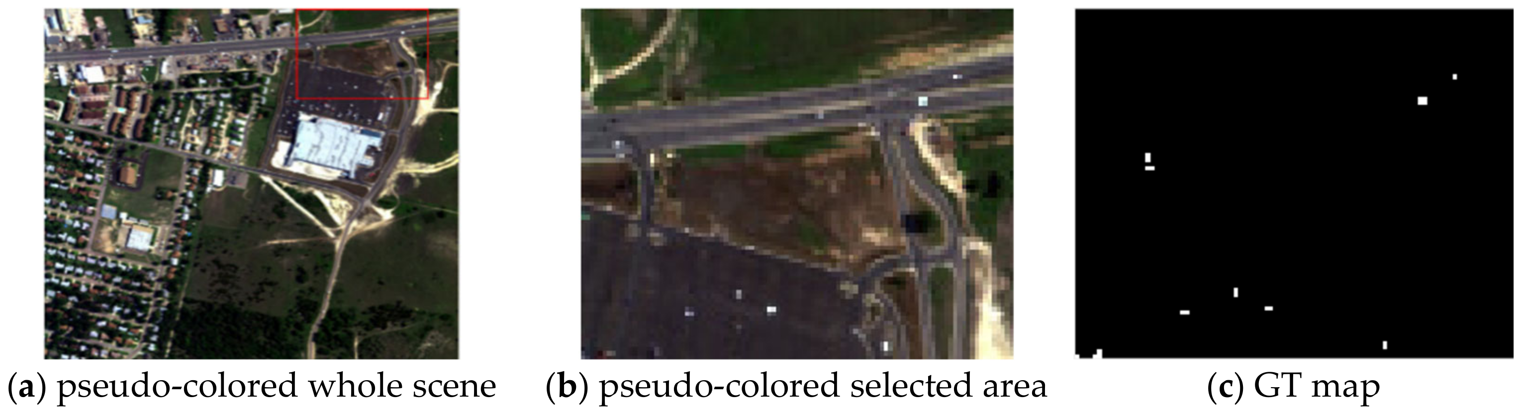
4.2. Data Set of Type II: Gainesville Data Scene

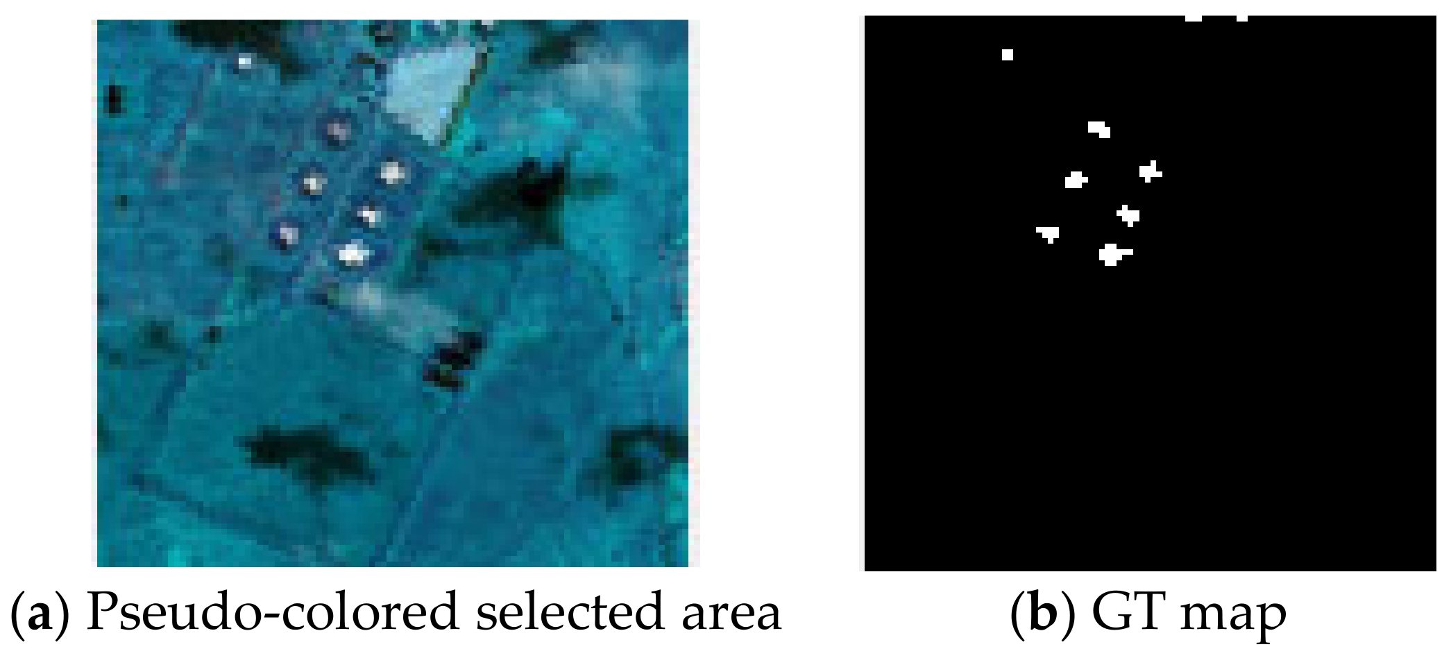
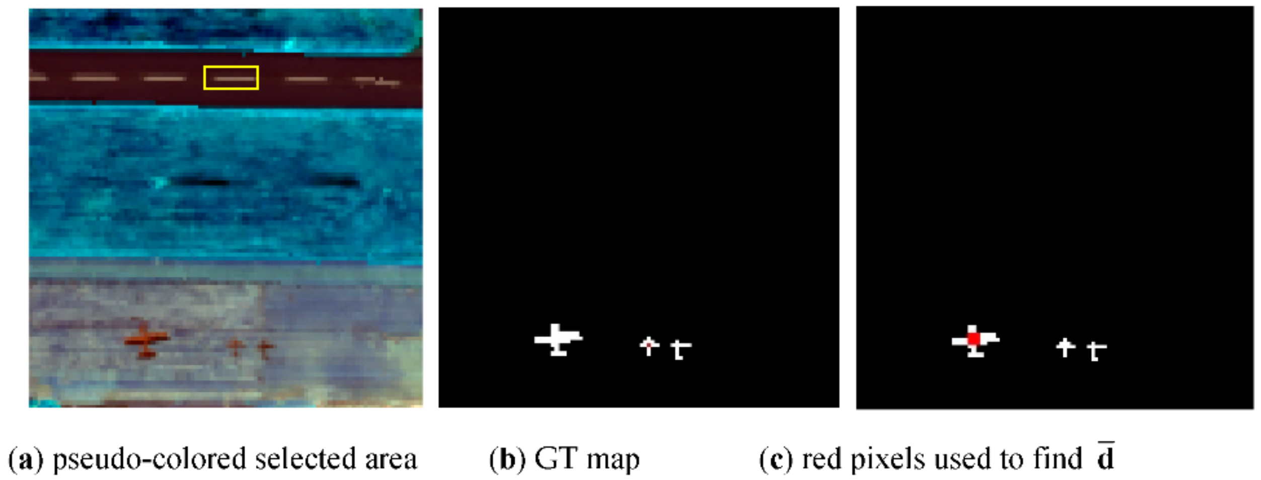
There are 11 targets in Gainesville data scene in Figure 28a which are small but visible. Table 9 tabulates the size of each target specified by the number of pixels according to the GT.
So, by inspection of Figure 28a according to GT in Figure 28b we performed PSTD by selecting a center pixel from each target highlighted by red in Figure 28c. As a result, a total of 11 pixels out of the 52 GT pixels obtained from Figure 28b were averaged to generate the desired target signature d ¯ used for CEM in (27).
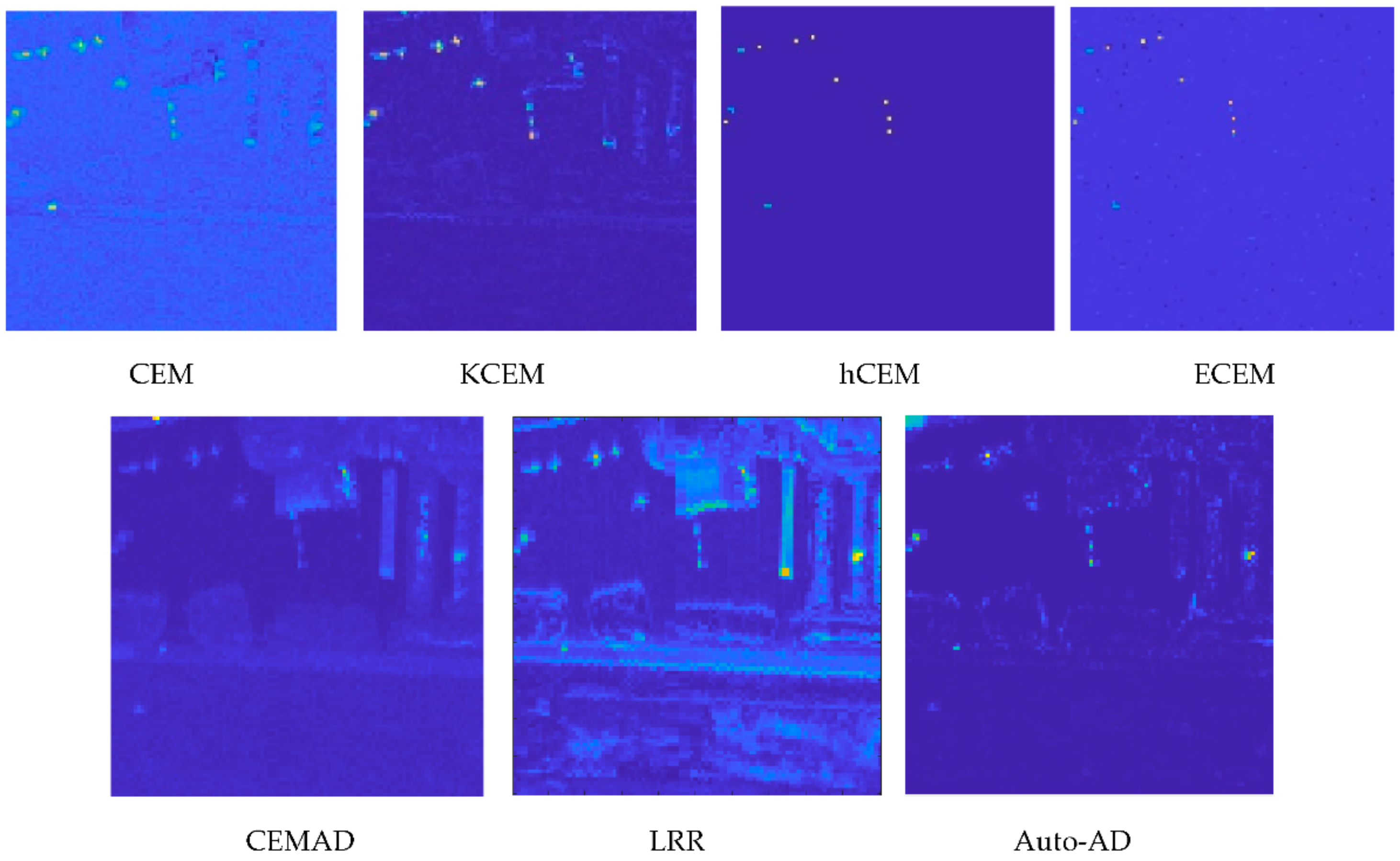
Figure 29 shows the detection maps of 11 targets produced by the CEM, KCEM, hCEM and ECEM with d ¯ used as the desired target signature.
By visual inspection of Figure 29, the KCEM was the best to detect all targets with very good BS, while the CEM could also detect all targets with slightly poor BS. Interestingly, the hCEM had best BS followed by the ECEM, both of which detected all target pixels that were used to calculate d ¯ , but they also over-suppressed all other target pixels.
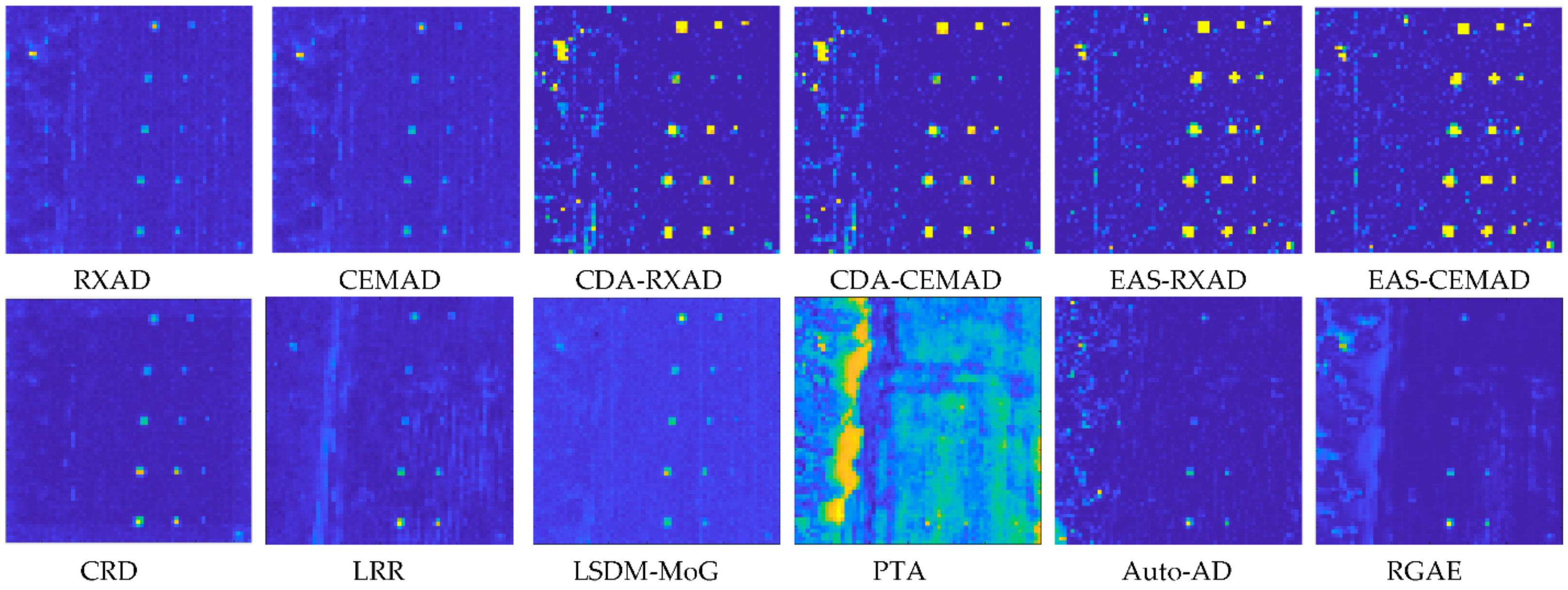
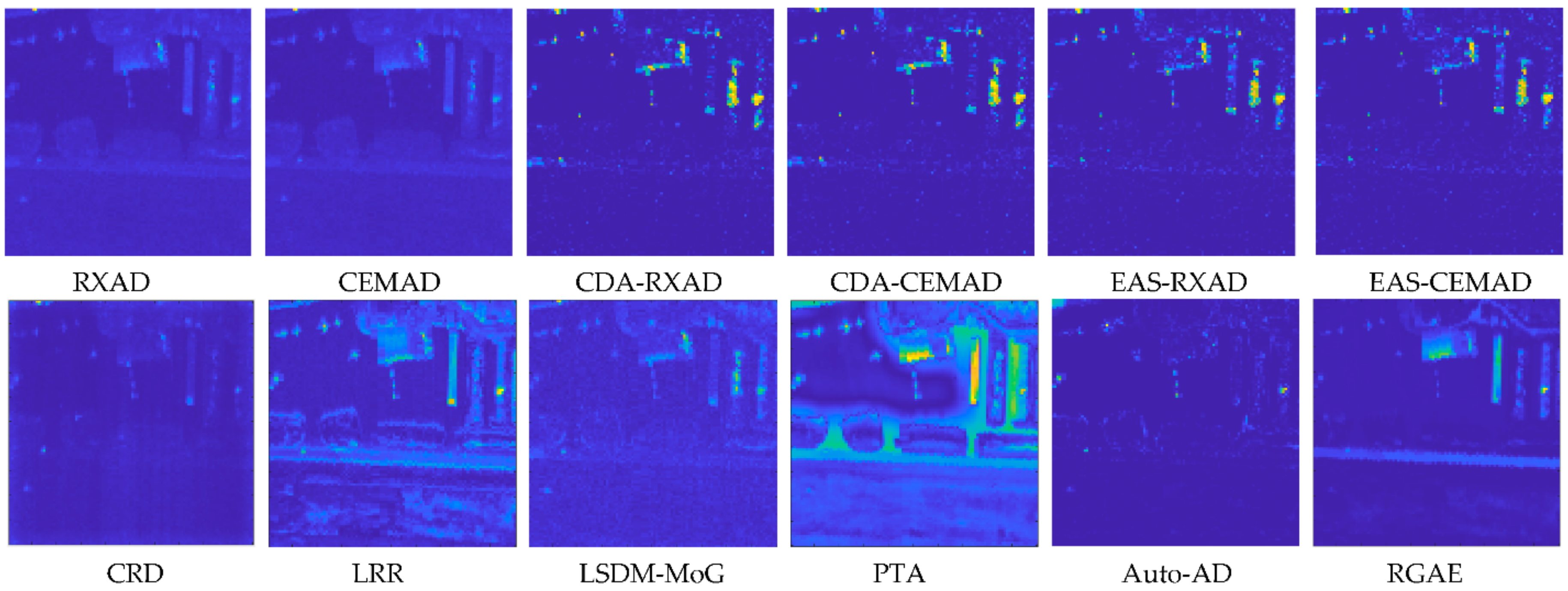
To compare AD, also included in Figure 29 are AD maps reproduced from Figure 13 by the best anomaly detectors, the LRR corresponding to the KCEM and Auto-AD corresponding to the hCEM and ECEM along with the CEMAD corresponding to the CEM for comparison. As we can see from Figure 29, TD using target information obtained by visual inspection performed much better than AD without using target knowledge. This is mainly due to the fact that PSTD knows exactly what targets it intends to detect, opposed to AD which detects all targets simultaneously as an anomaly detector without using any target knowledge. This is justified by evidence that the CEMAD, LRR and Auto-AD also picked up many of the BKG pixels as anomalies. For example, the CEM could detect all the target pixels using d ¯ compared to its corresponding anomaly detector counterpart, CEMAD without using d ¯ which detected all the target pixels weakly but also picked up the BKG pixels in the upper-right quadrant. As another example, the LRR was the best anomaly detector in terms of target detectability. But when compared to the best target detector, KCEM, the LRR detected quite a few of the BKG pixels. On the other hand, hCEM and ECEM performed excellent BS by only detecting the target pixels used to generate target information, d ¯ . Their corresponding anomaly detector counterpart is Auto-AD which also performed best BS. However, Auto-AD still could not compete against hCEM and ECEM in terms of cleaning up the BKG.
To further visualize this, Table 10 tabulates the eight TD measures using (48)–(52) where the best results for PSTD and AD boldfaced by black and red, respectively. It is very clear that the KCEM was the best with six out of eight quantitative measures, whereas hCEM was the worst in target detectability but best in BS. For comparison, Table 10 also tabulates eight AD measures produced by the CEMAD, LRR, Auto-AD and running times for Gainesville Scene where the AD-based AUC values produced by the CEMAD, LRR and Auto-AD in Table 4 are reinterpreted as TD-based AUC values by AUCADP = AUC(D), AUCBDP = 1 − AUC(F), AUCJAD = AUC(D,F) + AUC(D), AUCJBS = AUC(D,F) + 1 − AUC(F), AUCADBS = AUCTDBS, AUCSBPR = AUCSNPR and AUCOAD = AUC(D) + 1 − AUC(F), i.e., AUCOAD = 1 + AUCODP − AUC(D,F). The quantitative comparison in Figure 29 between PSTD and AD shows that the best PSTD did better than its corresponding anomaly detector counterpart across board with notable discrepancy. Nevertheless, their difference may not be that much.

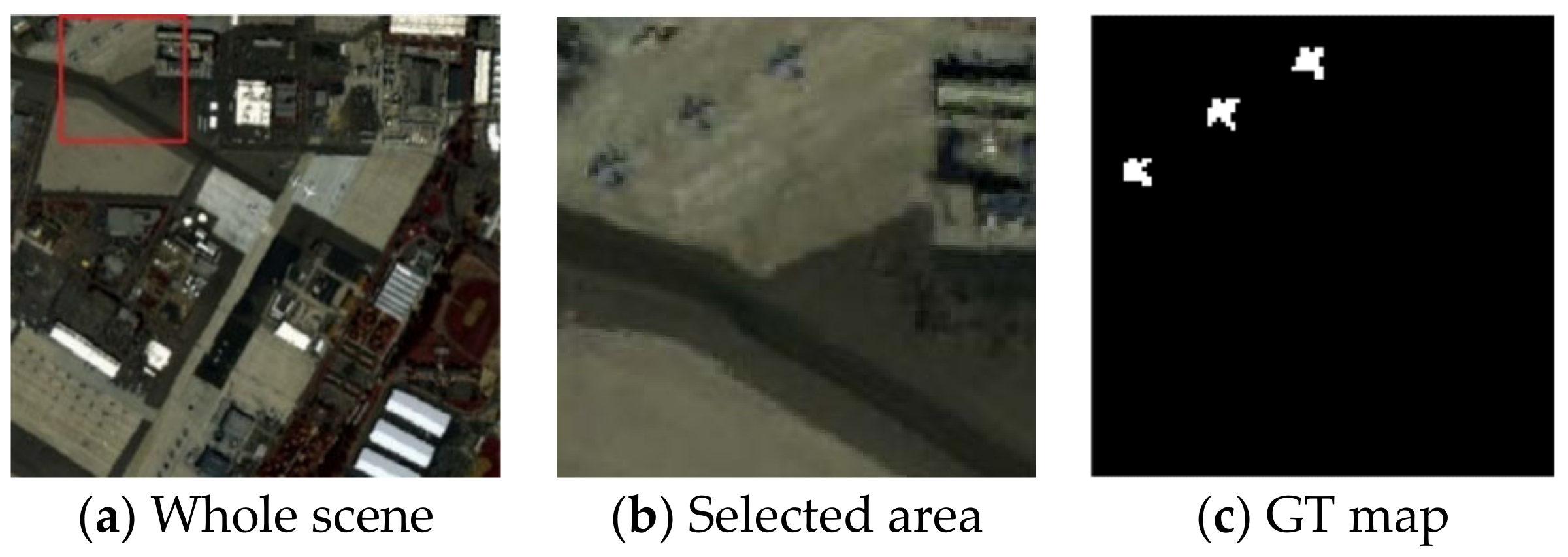
4.3. Data Set of Type III: Gulfport Scene

The San Diego Airport scene in Figure 4 was one of most widely used datasets for AD and has been studied extensively in the literature. Its inappropriateness furfure use in AD was discussed in great detail in ([10], Section VIII). To avoid duplication, this section investigates another similar but rather interesting data scene, Gulfport in 
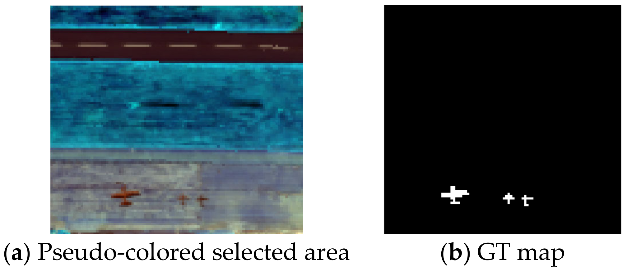
Figure 30a which also has three airplanes, one large and two small airplanes at the bottom but has a runway at the top part of the scene which was absent in the San Diego Airport data scene. By visual inspection, this runway should not be considered to be an anomaly but rather a specific target object. Accordingly, a detector which detects runway should not be considered for use as an anomaly detector. Two scenarios of PSTD were studied for this scene, one for detection of three airplanes and the other for detection of the runway.
  • Scenario 1: detection of the three airplanes.
Figure 30b shows its GT map along with Figure 30c which selected the pixels highlighted by red. These red pixels were averaged to be used as the desired target signature d ¯ for d used for CEM in (27). 
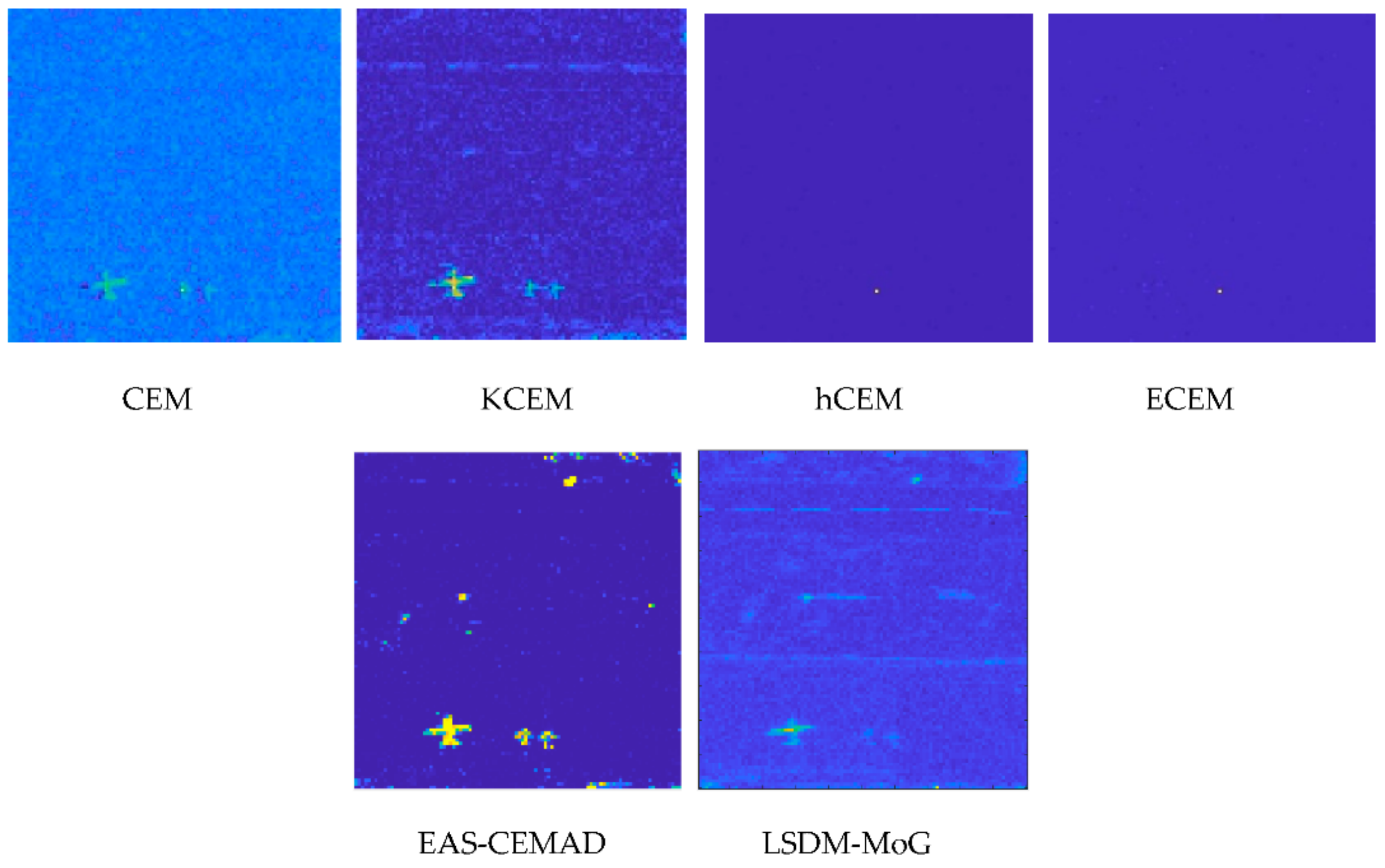
Figure 31 shows the detection maps of the CEM, KCEM, hCEM and ECEM. From the visual inspection of Figure 31, it is interesting to note that the KCEM clearly detected all the three airplanes plus the center line of the runway compared to the CEM, which also detected the three airplanes weakly but did not detect the runway. As for hCEM and ECEM, they were very sensitive to the used target knowledge and only detected those pixels used to obtain the d for CEM.
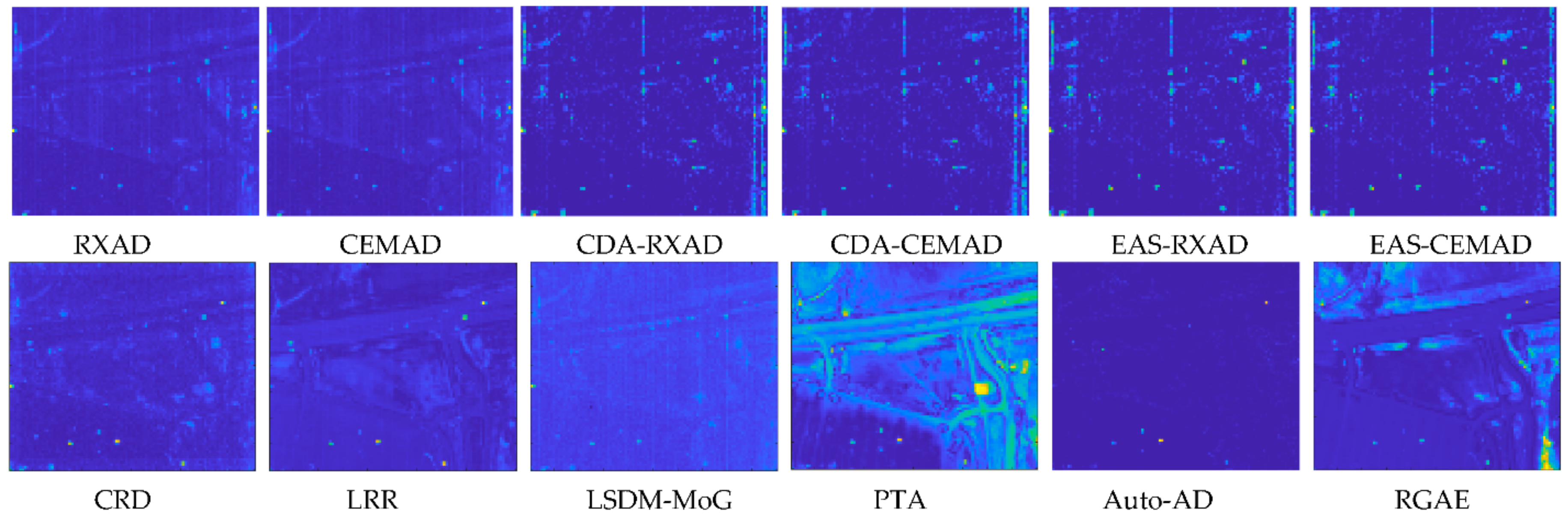
To further compare AD, we also reproduced the AD maps from Figure 17 and included them in Figure 31 for comparison with EAS-CEMAD corresponding to CEM and LSDM-MoG corresponding to KCEM most closely by visual inspection where EAS-CEMAD detected the three airplanes but did not detect the runway and LSDM-MoG detected the airplanes as well as the runway.
As we visually inspected the detection maps in Figure 31, it seemed that the best detector to detect all the three airplanes was EAS-CEMAD with the best AUC(F,τ), AUCBS, AUCTDBS and AUCSBPR, and not the CEM-based target detectors. However, Table 11 tabulates the detection maps in Figure 31 using the eight TD measures including (47)–(51) where the best results for PSTD and AD boldfaced by black and red, respectively. We immediately found that the conclusions made from the visual inspection of Figure 30 may not be true. As a matter of fact, the detector with best TD was CEM. On the other hand, KCEM achieved the best BS with highest values of AUCBS and AUCSBPR where EAS-CEMAD achieved the best AUCTDBS and AUCOAD.
  • Scenario 2: detection of runway.
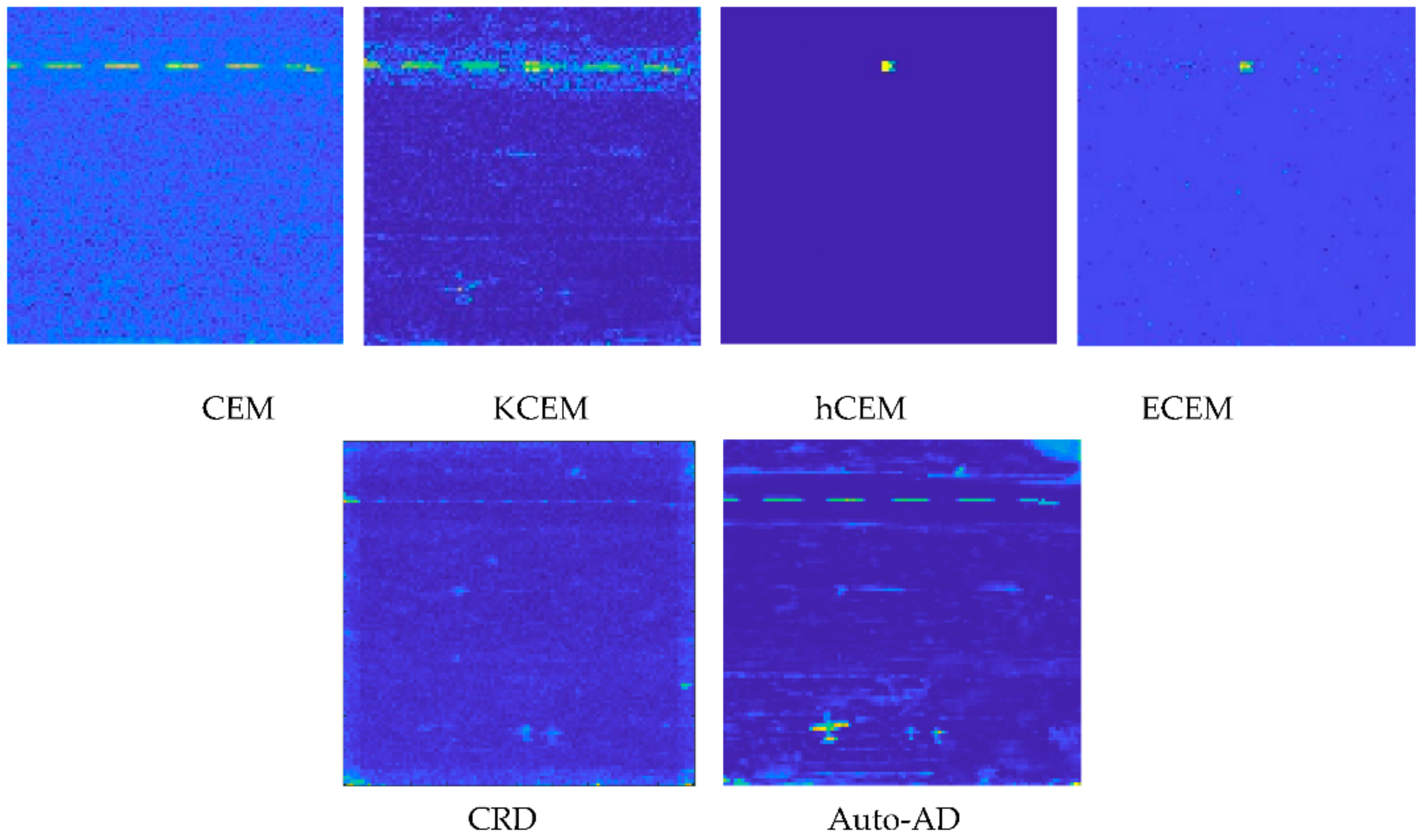
Using the small area of the center line in the runway highlighted by yellow in Figure 31a, Figure 32 shows the detection maps of the runway produced by CEM, KCEM, hCEM and ECEM. It clearly showed that CEM was the best and even performed better than KCEM, hCEM and ECEM. This was mainly due to the fact that KCEM, hCEM and ECEM were very sensitive to the pixels selected to calculate the desired target signature d. Also included in Figure 32 are the two corresponding anomaly detectors, CRD and Auto-AD reproduced from Figure 17 which yielded the best match the TD maps of CEM and KCEM, respectively by visual inspection. As long as the runway detection is concerned, Auto-AD outperformed all the target detectors and anomaly detectors in the visual inspection even Auto-AD did not use the runway signatures as target knowledge.
As a summary, the Gulfport scene produced mixed results. It is a good dataset for PSTD, but not AD where PSTD used a posteriori target knowledge obtained directly from the data by visual inspection without prior knowledge. This is because the GT used for the AD includes only three airplanes without a runway. According to the detection maps in 
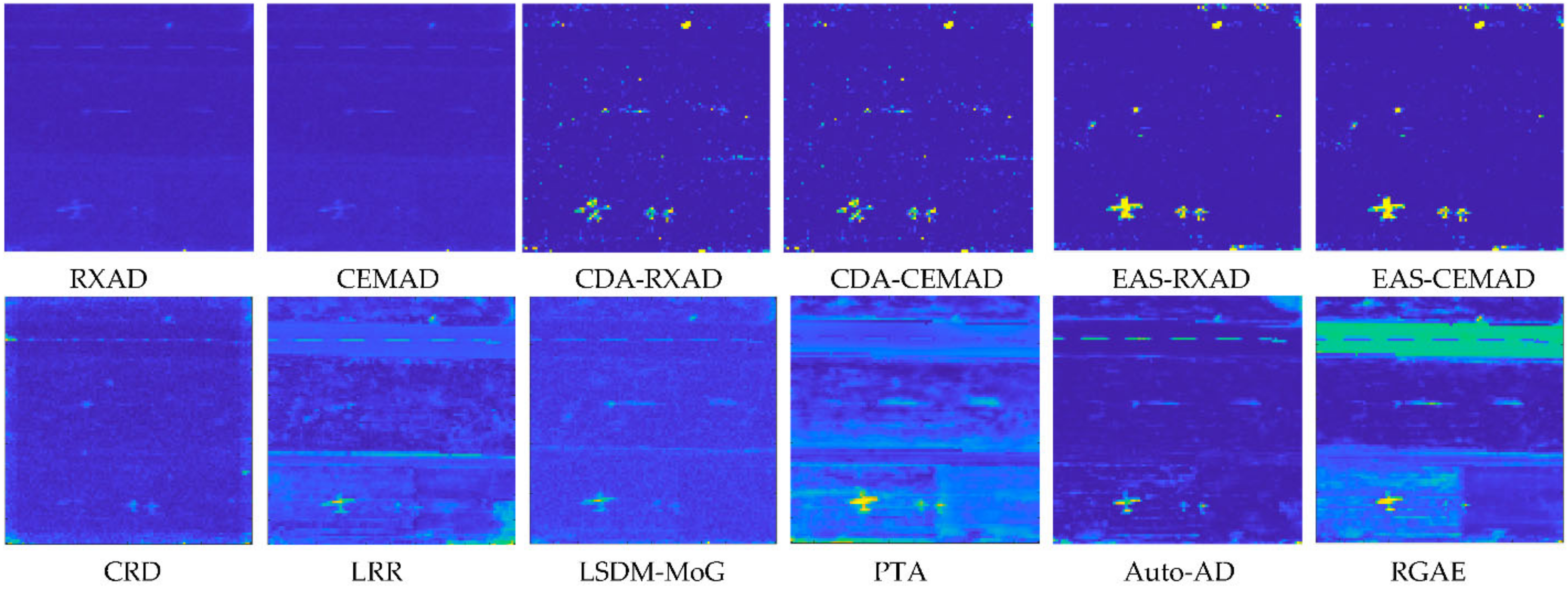
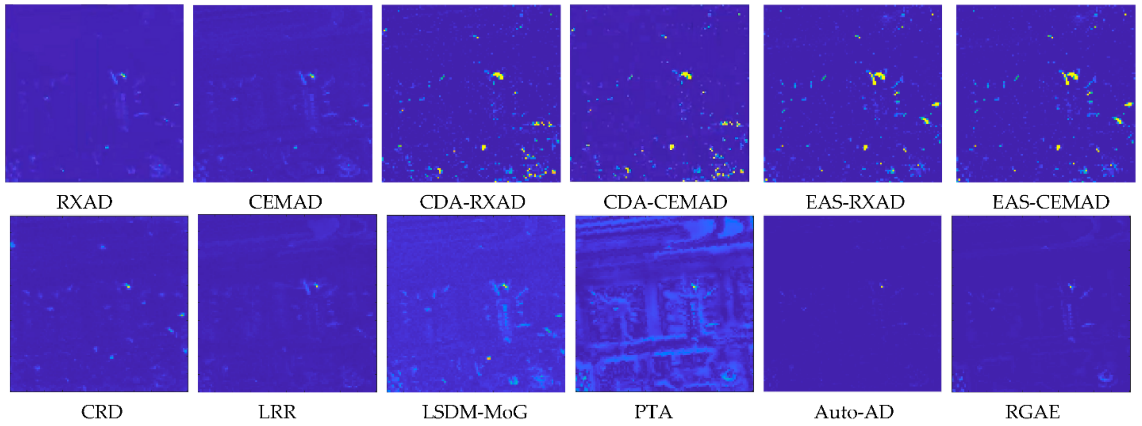
Figure 17, half of 12 test anomaly detectors, RXAD/CEMAD, CDA-RXAD/CEMAD and EAS-RXAD/CEMAD, did not detect the runway but the other half, CRD, LRR, LSDM-MoG, PTA, Auto-AD and RGAE did. So, if the provided GT does not include the runway, EAS-RXAD/CEMAD were the best. On the other hand, if the GT includes the runway, Auto-AD was clearly the only winner.

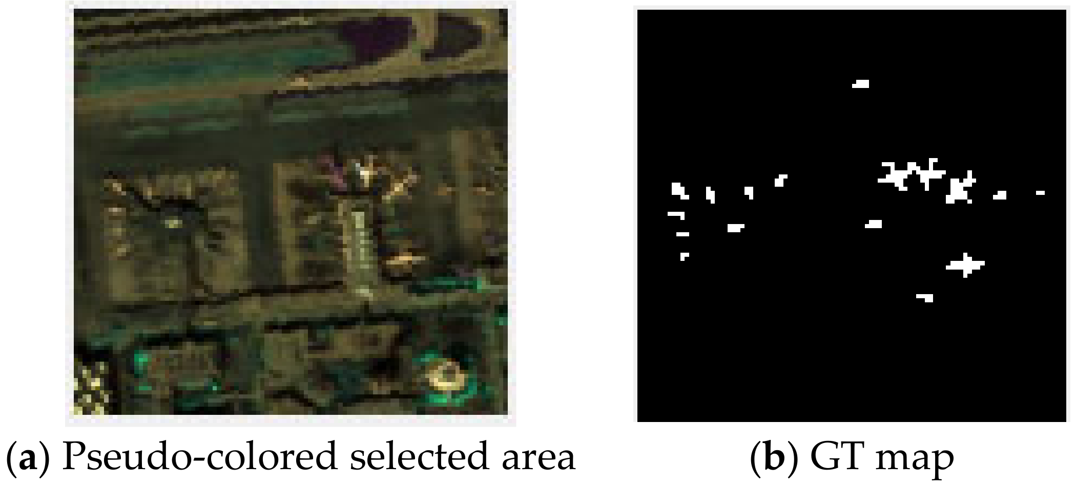
4.4. Data Set of Type IV: Los Angeles Scene

In Section 3.5.4 the AD maps of the Los Angeles dataset in Figure 7a produced by 12 test anomaly detectors yielded two sets of completely different detection results shown in Figure 26a and Figure 27a. In this section, we investigated the PSTD on the Los Angeles scene further by taking advantage of visual inspection to obtain target knowledge for target detectors, CEM, KCEM, hCEM and ECEM. This scene has two sets of targets of interest, small airplanes and large airplanes. Table 12 and Table 13 tabulates the size of each target specified by the number of pixels according to the GT in Figure 7a and Figure 7b respectively.
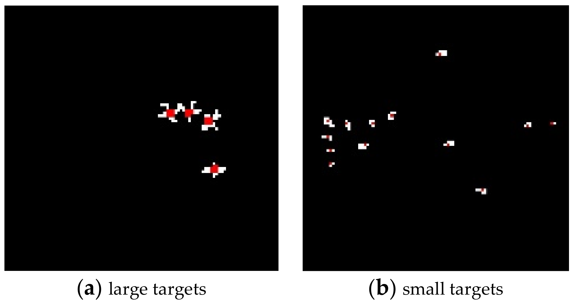
According to GT in Figure 7b align with our visual inspection, we selected 3 × 3 center pixels from each of large targets and a center pixel from each of small targets highlighted in red shown in Figure 33a,b, respectively. Then, these selected red pixels obtained in Figure 33a,b were averaged to generate the desired target signature d ¯ used for CEM in (27).
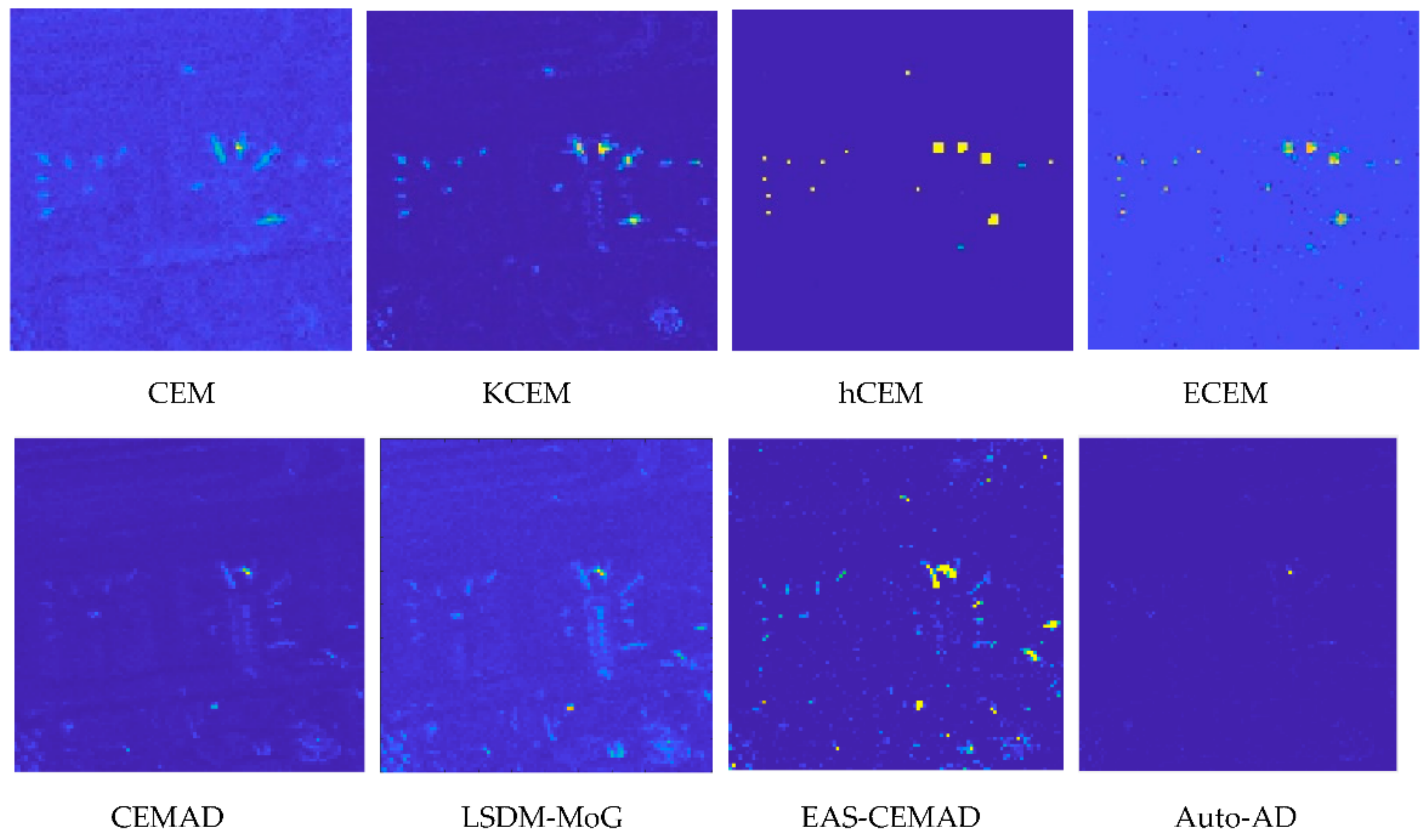
Figure 34 shows the detection maps of 11 targets produced by CEM, KCEM, hCEM and ECEM with d ¯ used as the desired target signature where 47 out of the 170 GT pixels for small and large targets selected from Figure 33a,b were averaged to calculate d ¯ .
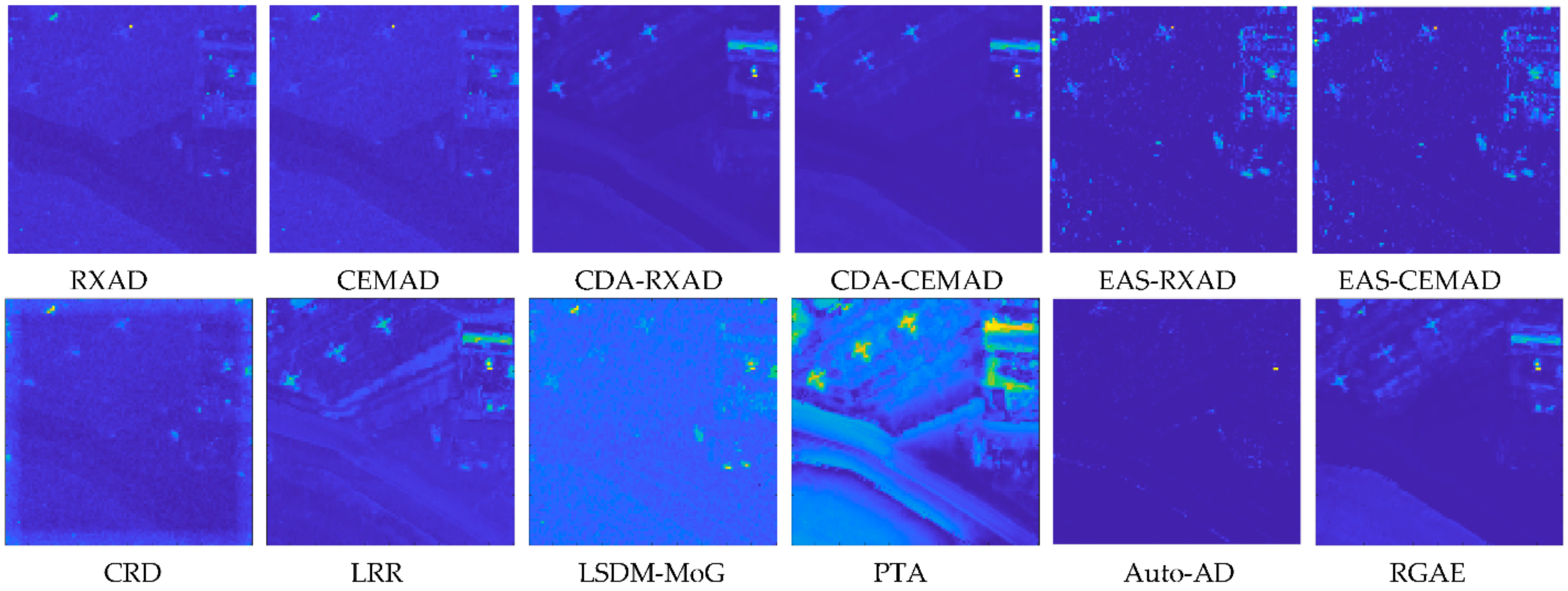
To compare AD, we examined the detection maps in Figure 34 and tried to identify the best possible anomaly detectors that produced AD maps to best match the detection maps produced by CEM, KCEM, hCEM and ECEM it turns out to be LSDM-MoG corresponding to KCEM, EAS-CEMAD corresponding to hCEM, Auto-AD corresponding to ECEM along with CEMAD corresponding to CEM. As we can see from Figure 34, PSTD using a posteriori target information obtained by visual inspection performed much better than its corresponding counterpart AD without using target knowledge. This is because PSTD knows exactly what targets it intended to detect by using a posteriori target knowledge compared to AD which detects all targets all at once as an anomaly detector without knowing any target knowledge. Like Table 11, Table 14 tabulates the detection maps in Figure 34 using the eight TD measures (47)–(51) where the best results for PSTD boldfaced by black. It is very clear to show that KCEM was the best with four out of the eight qualitative measures, while the ECEM was the worst in target detectability. In addition, the hCEM and ECEM also performed the best in BS. In order to make comparison with Table 8, Table 14 also tabulates the eight AD measures produced by the CEMAD, LSDM-MoG, EAS-CEMAD and Auto-AD in terms of the TD measures and running times where the best result for AD are boldfaced by red. The quantitative comparison in Table 14 between the TD and AD shows that the best target detector did better than its corresponding anomaly detector counterpart across board with notable discrepancy except AUC(F) which was only slightly worse within 10−2 range.
From Figure 34, CEM detected nearly all the target pixels using d ¯ compared to its corresponding anomaly detector counterpart, CEMAD without using d ¯ which weakly detected the center pixels of the second large airplane. Also, Table 14 shows that there is no comparison between the best target detector, KCEM, and the best anomaly detector, LSDM-MoG. It is interesting to see that compared to hCEM, EAS-CEMAD performed relatively well in detecting small targets including small airplanes, while missing a large part of large targets. This is exactly what an anomaly detector is expected to do. Moreover, the EAS-CEMAD also achieved reasonably good results in BS compared to hCEM and ECEM. It is also worth noting that both hCEM and ECEM clearly detected the target pixels used to generate target information, d ¯ with very good BS, whereas their corresponding anomaly detector counterparts are (i) EAS-CEMAD, which performed well in BS but also produced many falsely alarmed target pixels, and (ii) Auto-AD, which over-suppressed the BKG at the expense of missing nearly all target pixels.

5. Conclusions

Over the past few years, many AD methods have been developed in the literature and their goodness and effectiveness have been justified by two key elements, datasets and performance measures. Unfortunately, the issue of appropriateness of datasets used for AD was first realized in [10] but was no further explored. As a matter of fact, such inappropriate use of datasets is actually caused by their provided GTs which do not identify many unknown objects as anomalies as demonstrated in Section 3.5.3 and Section 3.5.4. Unfortunately, this issue has never been investigated in the past. In addition, the conventional 2D ROC curve used as an evaluation tool was also shown to be ineffective [16,18]. This paper investigates these two issues by conducting a comprehensive analysis using extensive experiments with seven popular datasets commonly used for AD. Specifically, the area of 2D ROC curve of PD versus PF, AUC(D,F) used in the traditional 2D ROC analysis was expanded to eight 3D ROC curve-derived AD measures which offer better and more effective criteria to evaluate AD performance in terms of anomaly detectability and BS. To further demonstrate the appropriateness of datasets used for AD, the experiments are also included in the performance of a comparative analysis between PSTD, which uses a posteriori target knowledge using visual inspection, and AD, which does use any target knowledge. According to the conducted experiments, it turns out that most widely used datasets for the evaluation of anomaly detectors in the literature are indeed not appropriate for AD, but better for PSTD.
It should be also noted that the main goal of this paper is to provide evidence and to further to show that datasets and performance measures are crucial to evaluate whether a detector can be considered for use as an anomaly detector. To the authors’ best knowledge, datasets used for experiments and detection measures used for performance evaluation are two issues needed to be addressed in the current AD research society. This can be seen in many works published in recent years. Unfortunately, very little has been conducted for it. As for future research avenues resulting from this paper, three directions may be worth investigating. One is how to distinguish PSTD from AD. As demonstrated in the experiments conducted in this paper, many detectors claimed to be anomaly detectors are indeed unsupervised a posteriori target detectors and are not really anomaly detectors. The experiments also show that statistical-based detectors are more likely to incline to anomaly detectors, while training sampling-based DL detectors to work more like unsupervised a posteriori target detectors. It is worth exploring their differences. A second direction is to investigate anomaly detectability and BS, which are completely different concepts that can be addressed by PD and 1-PF used in 3D ROC analysis. A third one is how to make an unsupervised a posteriori target detector a hyperspectral anomaly detector [72,73].

Author Contributions

Conceptualization, C.-I.C.; methodology, C.-I.C.; software, S.C.; validation, S.C., Y.S. and S.Z.; formal analysis, S.C. and S.Z.; investigation, S.C. and Y.S.; writing—C.-IC.; writing—review and editing, C.-I.C. All authors have read and agreed to the published version of the manuscript.

Funding

The work of C.-I Chang was partly supported by National Science and Technology Council (NSTC) under Grant 111-2634-F-006-012. The work of S. Zhong was in part supported by the National Natural Science Foundation (NSF) of China under grant 62101261, the NSF of Jiangsu Province under grant BK20210332.

Data Availability Statement

Data are contained within the article.

Acknowledgments

The work of Chein-I Chang is supported by YuShan Fellow Program sponsored by Ministry of Education in Taiwan.

Conflicts of Interest

The authors declare no conflicts of interest.

Correction Statement

This article has been republished with a minor correction to the existing affiliation information. "The University of Maryland, Baltimore" should change to "The University of Maryland, Baltimore County". This change does not affect the scientific content of the article.

References

  1. Chang, C.-I. Hyperspectral Imaging: Techniques for Spectral Detection and Classification; Kluwer Academic; Plenum Publishers: Dordrecht, The Netherlands, 2003. [Google Scholar]
  2. Chang, C.-I. Real-Time Progressive Hyperspectral Image Processing: Endmember Finding and Anomaly Detection; Springer: New York, NY, USA, 2016. [Google Scholar]
  3. Chang, C.-I. Hyperspectral Anomaly Detection Theory: A Dual Theory of Hyperspectral Target Detection. IEEE Trans. Geosci. Remote Sens. 2022, 60, 5511720. [Google Scholar] [CrossRef]
  4. Reed, I.S.; Yu, X. Adaptive Multiple-Band CFAR Detection of an Optical Pattern with Unknown Spectral Distribution. IEEE Trans. Acoust. Speech Signal Process. 1990, 38, 1760–1770. [Google Scholar] [CrossRef]
  5. Chang, C.-I.; Lin, C.-Y.; Chung, P.C.; Hu, P. Iterative Spectral-Spatial Hyperspectral Anomaly Detection. IEEE Trans. Geosci. Remote Sens. 2023, 61, 5504330. [Google Scholar] [CrossRef]
  6. Xu, Y.; Wu, Z.; Li, J.; Plaza, A.; Wei, Z. Anomaly Detection in Hyperspectral Images Based on Low-Rank and Sparse Representation. IEEE Trans. Geosci. Remote Sens. 2016, 54, 1990–2000. [Google Scholar] [CrossRef]
  7. Zhou, T.; Tao, D. GoDec: Randomized Low-Rank and Sparsity Matrix Decomposition in Noisy Case. In Proceedings of the 28th International Conference on Machine Learning, Bellevue, WA, USA, 28 June–2 July 2011. [Google Scholar]
  8. Zhang, X.; Wen, G.; Dai, W. A Tensor Decomposition-based Anomaly Detection Algorithm for Hyperspectral Image. IEEE Trans. Geosci. Remote Sens. 2016, 54, 5801–5820. [Google Scholar] [CrossRef]
  9. Hu, X.; Xie, C.; Fan, Z.; Duan, Q.; Zhang, D.; Jiang, L.; Wei, X.; Hong, D.; Li, G.; Zeng, X.; et al. Hyperspectral Anomaly Detection Using Deep Learning: A Review. Remote Sens. 2022, 14, 1973. [Google Scholar] [CrossRef]
  10. Chang, C.-I. Effective Anomaly Space for Hyperspectral Anomaly Detection. IEEE Trans. Geosci. Remote Sens. 2022, 60, 5526624. [Google Scholar] [CrossRef]
  11. Hyvarinen, A.; Karhunen, J.; Oja, E. Independent Component Analysis; John Wiley & Sons: Hoboken, NJ, USA, 2001. [Google Scholar]
  12. Chen, S.; Chang, C.-I.; Li, X. Component decomposition analysis for hyperspectral target detection. IEEE Trans. Geosci. Remote Sens. 2022, 60, 1–22. [Google Scholar]
  13. Zhong, J.; Xie, W.; Li, Y.; Lei, J.; Du, Q. Characterization of Background-Anomaly Separability with Generative Adversarial Network for Hyperspectral Anomaly Detection. IEEE Trans. Geosci. Remote Sens. 2021, 59, 6017–6028. [Google Scholar] [CrossRef]
  14. Wu, Z.; Zhu, W.; Chanussot, J.; Xu, Y.; Osher, S. Hyperspectral Anomaly Detection Via Global and Local joint Modeling of Background. IEEE Trans. Signal Process. 2019, 67, 3858–3869. [Google Scholar] [CrossRef]
  15. Jiang, T.; Li, Y.; Xie, W.; Du, Q. Discriminative Reconstruction Constrained Generative Adversarial Network for Hyperspectral Anomaly Detection. IEEE Trans. Geosci. Remote Sens. 2020, 58, 4666–4679. [Google Scholar] [CrossRef]
  16. Chang, C.-I. An Effective Evaluation Tool for Hyperspectral Target Detection: 3D Receiver Operating Characteristic Analysis. IEEE Trans. Geosci. Remote Sens. 2021, 59, 5131–5153. [Google Scholar] [CrossRef]
  17. Poor, H.V. An Introduction to Signal Detection and Estimation; Springer: New York, NY, USA, 1991. [Google Scholar]
  18. Chang, C.-I. Comprehensive Analysis of Receiver Operating Characteristic ROC Curves for Hyperspectral Anomaly Detection. IEEE Trans. Geosci. Remote Sens. 2022, 60, 5541124. [Google Scholar] [CrossRef]
  19. Candes, E.J.; Li, X.; Ma, Y.; Wright, J. Robust Principal Component Analysis? J. ACM 2009, 58, 1027–1063. [Google Scholar] [CrossRef]
  20. Vaswani, N.; Bouwmans, T.; Javed, S.; Narayanamurth, P. Robust Subspace Learning: Robust PCA, Robust Subspace Tracking and Robust Subspace Recovery. IEEE Signal Process. Mag. 2018, 35, 32–55. [Google Scholar] [CrossRef]
  21. Sobral, A.; Bouwmans, T.; Zahzah, E. (Eds.) LRSLibrary: Low-Rank and Sparse Tools for Background Modeling and Subtraction in Videos. In Handbook of Robust Low-Rank and Sparse Matrix Decomposition: Applications in Image and Video Processing, 1st ed.; Chapman and Hall; CRC: Boca Raton, FL, USA, 2016. [Google Scholar]
  22. Li, L.; Li, W.; Qu, Y.; Zhao, C.; Tao, R.; Du, Q. Prior-Based Tensor Approximation for Anomaly Detection in Hyperspectral Imagery. IEEE Trans. Neural Netw. Learn. Syst. 2022, 33, 1037–1050. [Google Scholar] [CrossRef] [PubMed]
  23. Wang, S.; Wang, X.; Zhang, L.; Zhong, Y. Deep Low Rank Prior for Hyperspectral Anomaly Detection. IEEE Trans. Geosci. Remote Sens. 2022, 60, 5527017. [Google Scholar] [CrossRef]
  24. Li, X.; Yuan, Y. A Tensor-based Hyperspectral Anomaly Detection under Prior Physical Constraint. IEEE Trans. Geosci. Remote Sens. 2023, 61, 2023. [Google Scholar] [CrossRef]
  25. Li, H.; Tang, J.; Zhou, H. Hyperspectral Anomaly Detection Based Joint Multi-Feature Trilateral Filtering and Collaborative Representation. Appl. Sci. 2024, 13, 6943. [Google Scholar] [CrossRef]
  26. Chang, C.-I. Hyperspectral Target Detection: Hypothesis Testing, Signal-to-Noise Ratio and Spectral Angle Theories. IEEE Trans. Geosci. Remote Sens. 2022, 60, 5505223. [Google Scholar] [CrossRef]
  27. Manolakis, D.; Pieper, M.; Truslow, E.; Cooley, T.; Brueggeman, M.; Lipson, S. The Remarkable Success of Adaptive Cosine Estimator in Hyperspectral Target Detection. In Proceedings of the SPIE, Algorithms and Technologies for Multispectral, Hyperspectral, and Ultraspectral Imagery XIX, Baltimore, MD, USA, 29 April–2 May 2013; Volume 8743, p. 874302-1-13. [Google Scholar]
  28. Stein, D.W.J.; Beaven, S.G.; Hoff, L.E.; Winter, E.M.; Schaum, A.P.; Stocker, A.D. Anomaly Detection from Hyperspectral Imagery. IEEE Signal Process. Mag. 2020, 19, 58–69. [Google Scholar] [CrossRef]
  29. Manolakis, D.; Truslow, E.; Pieper, M.; Cooley, T.; Brueggeman, M. Detection Algorithms in Hyperspectral Imaging systems. IEEE Signal Process. Mag. 2014, 31, 24–33. [Google Scholar] [CrossRef]
  30. Robey, F.C.; Fuhrmann, D.R.; Kelly, E.J.; Nitzberg, R. A CFAR Adaptive Matched Filter Detector. IEEE Trans. Aerosp. Electron. Syst. 1992, 28, 208–218. [Google Scholar] [CrossRef]
  31. Scharf, L.L.; Friedlander, B. Matched Subspace Detectors. IEEE Trans. Signal Process. 1994, 42, 2146–2157. [Google Scholar] [CrossRef]
  32. Chang, C.-I. Constrained Energy Minimization Anomaly Detection for Hyperspectral Imagery. IEEE Trans. Geosci. Remote Sens. 2020, 60, 1–19. [Google Scholar]
  33. Chang, C.-I.; Chiang, S.-S. Anomaly Detection and Classification for Hyperspectral Imagery. IEEE Trans. Geosci. Remote Sens. 2002, 40, 1314–1325. [Google Scholar] [CrossRef]
  34. Chang, C.-I. Real-Time Recursive Hyperspectral Sample and Band Processing: Algorithm Architecture and Implementation; Springer: Berlin/Heidelberg, Germany, 2017. [Google Scholar]
  35. Picinbono, B. On deflection as a performance criterion in detection. IEEE Trans. Aerosp. Electron. Syst. 1995, 31, 1072–1081. [Google Scholar] [CrossRef]
  36. Harsanyi, J.C. Detection and Classification of Subpixel Spectral Signatures in Hyperspectral Image Sequences. Ph.D. Thesis, Department of Electrical Engineering, University of Maryland Baltimore County, Baltimore, MD, USA, 1993. [Google Scholar]
  37. Molero, J.M.; Garzón, E.M.; García, I.; Plaza, A. Analysis and Optimizations of Global and Local Versions of the RX Algorithm for Anomaly Detection in Hyperspectral Data. IEEE J. Sel. Top. Appl. Earth Obs. Remote Sens. 2013, 6, 801–814. [Google Scholar] [CrossRef]
  38. Matteoli, T.; Veracini, T.; Diani, M.; Corsini, G. A Locally Adaptive Background Density Estimator: An Evolution for RX-based Anomaly Detectors. IEEE Geosci. Remote Sens. Lett. 2014, 11, 323–327. [Google Scholar] [CrossRef]
  39. Banerjee, A.; Burlina, P.; Diehl, C. A Support Vector Method for Anomaly Detection in Hyperspectral Imagery. IEEE Trans. Geosci. Remote Sens. 2020, 44, 2282–2291. [Google Scholar] [CrossRef]
  40. Guo, Q.; Zhang, B.; Ran, Q.; Gao, L.; Li, J.; Plaza, A. Weighted-RXD and Linear Filter-based RXD: Improving Background Statistics Estimation for Anomaly Detection in Hyperspectral Imagery. IEEE J. Sel. Top. Appl. Earth Obs. Remote Sens. 2020, 7, 2351–2366. [Google Scholar] [CrossRef]
  41. Chang, C.-I.; Wang, Y.; Chen, S.Y. Anomaly Detection Using Causal Sliding Windows. IEEE J. Sel. Top. Appl. Earth Obs. Remote Sens. 2015, 8, 3260–3270. [Google Scholar] [CrossRef]
  42. Kwon, H.; Der, S.Z.; Nasrabadi, N.M. Adaptive Anomaly Detection Using Subspace Separation for Hyperspectral Imagery. Opt. Eng. 2003, 42, 3342–3351. [Google Scholar] [CrossRef]
  43. Wei, L.; Du, Q. Collaborative Representation for Hyperspectral Anomaly Detection. IEEE Trans. Geosci. Remote Sens. 2015, 53, 1463–1474. [Google Scholar]
  44. Liu, W.; Chang, C.-I. Multiple Window Anomaly Detection for Hyperspectral Imagery. IEEE J. Sel. Top. Appl. Earth Obs. Remote Sens. 2013, 6, 644–658. [Google Scholar] [CrossRef]
  45. Tang, L.; Li, Z.; Wang, W.; Zhao, B.; Pan, Y.; Tian, Y. An Efficient and Robust Framework for Hyperspectral Anomaly Detection. Remote Sens. 2021, 13, 4247. [Google Scholar] [CrossRef]
  46. Lei, J.; Xie, W.; Yang, J.; Li, Y.; Chang, C.-I. Spectral–Spatial Feature Extraction for Hyperspectral Anomaly Detection. IEEE Trans. Geosci. Remote Sens. 2019, 57, 8131–8143. [Google Scholar] [CrossRef]
  47. Kwon, H.; Nasrabadi, N.M. Kernel RX-algorithm: A Nonlinear Anomaly Detector for Hyperspectral Imagery. IEEE Trans. Geosci. Remote Sens. 2005, 43, 388–397. [Google Scholar] [CrossRef]
  48. Wang, Y.; Lee, L.C.; Xue, B.; Wang, L.; Song, M.; Li, S.; Chang, C.-I. A Posteriori Hyperspectral Anomaly Detection for Unlabeled Classification. IEEE Trans. Geosci. Remote Sens. 2018, 56, 3091–3106. [Google Scholar] [CrossRef]
  49. Chen, S.Y.; Wang, Y.; Wu, C.C.; Liu, C.; Chang, C.-I. Real Time Causal Processing of Anomaly Detection in Hyperspectral Imagery. IEEE Trans. Aerosp. Electron. Syst. 2014, 50, 1511–1534. [Google Scholar] [CrossRef]
  50. Liu, J.; Hou, Z.; Li, W.; Tao, R.; Orlando, D.; Li, H. Multipixel Anomaly Detection with Unknown Patterns for Hyperspectral Imagery. IEEE Trans. Neural Netw. Learn. Syst. 2022, 33, 5557–5567. [Google Scholar] [CrossRef] [PubMed]
  51. Yuan, Y.; Ma, D.; Wang, Q. Hyperspectral Anomaly Detection by Graph Pixel Selection. IEEE Trans. Cybern. 2016, 46, 3123–3134. [Google Scholar] [CrossRef] [PubMed]
  52. Kang, X.; Zhang, X.; Li, S.; Li, K.; Li, J.; Benediktsson, J.A. Hyper-spectral Anomaly Detection with Attribute and Edge-Preserving Filters. IEEE Trans. Geosci. Remote Sens. 2017, 55, 5600–5611. [Google Scholar] [CrossRef]
  53. Qu, J.; Du, Q.; Li, Y.; Tian, L.; Xia, H. Anomaly Detection in Hyperspectral Imagery Based on Gaussian Mixture Model. IEEE Trans. Geosci. Remote Sens. 2021, 59, 9504–9617. [Google Scholar] [CrossRef]
  54. Ma, N.; Peng, Y.; Wang, S.; Leong, P.H.W. An Unsupervised Deep Hyperspectral Anomaly Detector. Sensors 2018, 18, 693. [Google Scholar] [CrossRef] [PubMed]
  55. Wang, X.; Wang, L.; Zhang, Y. Auto-AD: Autonomous Hyperspectral Anomaly Detection Network Based on Fully Convolutional Autoencoder. IEEE Trans. Geosci. Remote Sens. 2022, 60, 5503314. [Google Scholar] [CrossRef]
  56. Xiang, P.; Ali, S.; Jung, S.K.; Zhou, H. Hyperspectral Anomaly Detection with Guided Autoencoder. IEEE Trans. Geosci. Remote Sens. 2022, 60, 5538818. [Google Scholar] [CrossRef]
  57. Chen, S.; Li, X.; Yan, Y. Hyperspectral Anomaly Detection with Auto-Encoder and Independent Targets. Remote Sens. 2023, 15, 5266. [Google Scholar] [CrossRef]
  58. Xie, W.; Liu, B.; Li, Y.; Lei, J.; Du, Q. Autoencoder and Adversarial Learning-based Semisupervised Background Estimation for Hyperspectral Anomaly Detection. IEEE Trans. Geosci. Remote Sens. 2020, 58, 5416–5427. [Google Scholar] [CrossRef]
  59. Fan, G.; Ma, Y.; Mei, X.; Fan, F.; Huang, J.; Ma, J. Hyperspectral Anomaly Detection with Robust Graph Autoencoders. IEEE Trans. Geosci. Remote Sens. 2022, 60, 5511314. [Google Scholar] [CrossRef]
  60. Chang, S.; Du, B.; Zhang, L. BASO: A Background-Anomaly Component Projection and Separation Optimized filter for Anomaly Detection in Hyperspectral Images. IEEE Trans. Geosci. Remote Sens. 2018, 56, 3747–3761. [Google Scholar] [CrossRef]
  61. Li, L.; Li, W.; Du, Q.; Tao, R. Low-Rank and Sparse Decomposition with Mixture of Gaussian for Hyperspectral Anomaly Detection. IEEE Trans. Cybern. 2021, 51, 4363–4372. [Google Scholar] [CrossRef] [PubMed]
  62. Zhang, Y.; Du, B.; Zhang, L.; Wang, S. A Low-Rank and Sparse Matrix Decomposition-Based Mahalanobis Distance method for Hyperspectral Anomaly detection. IEEE Trans. Geosci. Remote Sens. 2020, 54, 1376–1389. [Google Scholar] [CrossRef]
  63. Chang, C.-I.; Chen, J. Hyperspectral Anomaly Detection by Data Sphering and Sparsity Density Peaks. IEEE Trans. Geosci. Remote Sens. 2022, 60, 5526321. [Google Scholar] [CrossRef]
  64. Chang, C.-I. Hyperspectral Data Processing: Algorithm Design and Analysis; Wiley: Hoboken, NJ, USA, 2013. [Google Scholar]
  65. Chang, C.-I.; Du, Q. Estimation of Number of Spectrally Distinct Spectral Signal Sources in Hyperspectral Imagery. IEEE Trans. Geosci. Remote Sens. 2004, 42, 608–619. [Google Scholar] [CrossRef]
  66. Chang, C.-I. A Review of Virtual Dimensionality for Hyperspectral Imagery. IEEE J. Sel. Top. Appl. Earth Obs. Remote Sens. 2018, 11, 1285–1305. [Google Scholar] [CrossRef]
  67. Chang, C.-I.; Xiong, W.; Wen, C.H. A Theory of High Order Statistics-based Virtual Dimensionality for Hyperspectral Imagery. IEEE Trans. Geosci. Remote Sens. 2014, 52, 188–208. [Google Scholar] [CrossRef]
  68. Kuybeda, O.; Malah, D.; Barzohar, M. Rank Estimation and Redundancy Reduction of High-Dimensional Noisy Signals with Preservation of Rare Vectors. IEEE Trans. Signal Process. 2007, 55, 5579–5592. [Google Scholar] [CrossRef]
  69. Jiao, X.; Chang, C.-I. Kernel-based Constrained Energy Minimization (KCEM). In Proceedings of the SPIE Conference on Algorithms and Technologies for Multispectral, Hyperspectral, and Ultraspectral Imagery XIV, Orlando, FL, USA, 16–20 March 2008. [Google Scholar]
  70. Zou, Z.; Shi, Z. Hierarchical Suppression Method for Hyperspectral Target Detection. IEEE Trans. Geosci. Remote Sens. 2016, 54, 330–342. [Google Scholar] [CrossRef]
  71. Zhao, R.; Shi, Z.; Zou, Z.; Zhang, Z. Ensemble-based Cascaded Constrained Energy Minimization for Hyperspectral Target Detection. Remote Sens. 2019, 11, 1310. [Google Scholar] [CrossRef]
  72. Su, H.; Wu, Z.; Zhang, H.; Du, Q. Hyperspectral Anomaly Detection: A Survey. Geosci. Remote Sens. Mag. 2021, 10, 64–90. [Google Scholar] [CrossRef]
  73. Chang, C.-I. Target-to-Anomaly Conversion for Hyperspectral Anomaly Detection. IEEE Trans. Geosci. Remote Sens. 2022, 60, 5540428. [Google Scholar] [CrossRef]
Figure 1. (a) A HYDICE15-panel scene which contains 15 panels; (b) GT map of spatial locations of 19 R panel pixels.
Remotesensing 16 00135 g001
Figure 2. HYDICE urban scene.
Remotesensing 16 00135 g002
Figure 3. Gainesville scene.
Remotesensing 16 00135 g003
Figure 4. San Diego airport scene.
Remotesensing 16 00135 g004
Figure 5. Gulfport scene.
Remotesensing 16 00135 g005
Figure 6. Texas coast scene.
Remotesensing 16 00135 g006
Figure 7. Los Angeles Scene.
Remotesensing 16 00135 g007
Figure 8. A flowchart of the proposed methodology.
Remotesensing 16 00135 g008
Figure 9. Detection maps produced by RXAD/CEMAD, CDA-RXAD/CEMAD, EAS-RXAD/CEMAD, LRR, LSDM-MoG, PTA, Auto-AD and RGAE for the HYDICE panel scene.
Remotesensing 16 00135 g009
Figure 10. 3D ROC curves generated from Figure 9 for HYDICE panel scene.
Remotesensing 16 00135 g010
Figure 11. Detection maps produced by RXAD/CEMAD, CDA-RXAD/CEMAD, EAS-RXAD/CEMAD, LRR, LSDM-MoG, PTA, Auto-AD, RGAE for HYDICE urban scene.
Remotesensing 16 00135 g011
Figure 12. 3D ROC curves generated from Figure 11 for the HYDICE urban scene.
Remotesensing 16 00135 g012
Figure 13. Detection maps produced by RXAD/CEMAD, CDA-RXAD/CEMAD, EAS-RXAD/CEMAD, LRR, LSDM-MoG, PTA, Auto-AD and RGAE for the Gainesville scene.
Remotesensing 16 00135 g013
Figure 14. 3D ROC curves generated from Figure 13 for the Gainesville scene.
Remotesensing 16 00135 g014
Figure 15. Detection maps produced by RXAD/CEMAD, CDA-RXAD/CEMAD, EAS-RXAD/CEMAD, LRR, LSDM-MoG, PTA, Auto-AD, RGAE for the San Diego airport scene.
Remotesensing 16 00135 g015
Figure 16. 3D ROC curves generated from Figure 15 for San Diego Airport scene.
Remotesensing 16 00135 g016
Figure 17. Detection maps produced by RXAD/CEMAD, CDA-RXAD/CEMAD, EAS-RXAD/CEMAD, LRR, LSDM-MoG, PTA, Auto-AD, RGAE for the Gulfport Scene.
Remotesensing 16 00135 g017
Figure 19. Detection maps produced by RXAD/CEMAD, CDA-RXAD/CEMAD, EAS-RXAD/CEMAD, LRR, LSDM-MoG, PTA, Auto-AD and RGAE for Texas coast scene.
Remotesensing 16 00135 g019
Figure 20. 3D ROC curves generated from Figure 19 for the Texas coast scene.
Remotesensing 16 00135 g020
Figure 21. Detection maps produced by the RXAD/CEMAD, CDA-RXAD/CEMAD, EAS-RXAD/CEMAD, LRR, LSDM-MoG, PTA, Auto-AD, RGAE for the Los Angeles scene.
Remotesensing 16 00135 g021
Figure 22. 3D ROC curves generated from Figure 21 for the Los Angeles scene.
Remotesensing 16 00135 g022
Figure 23. An uninteresting two-pixel anomaly in the HYDICE panel scene in Figure 1a.
Remotesensing 16 00135 g023
Figure 24. An uninteresting two-pixel anomaly in the San Diego Airport scene in Figure 4b.
Remotesensing 16 00135 g024
Figure 25. Gainesville scene with the BKG.
Remotesensing 16 00135 g025
Figure 26. The Los Angeles Scene.
Remotesensing 16 00135 g026
Figure 27. Los Angeles Scene.
Remotesensing 16 00135 g027
Figure 28. The Gainesville scene along with the GT map and red pixels used to generate the target information.
Remotesensing 16 00135 g028
Figure 29. TD maps produced by the CEM, KCEM, hCEM and ECEM using d ¯ as the desired target signature and AD maps produced by CEMAD, LRR and Auto-AD.
Remotesensing 16 00135 g029
Figure 30. The Gulfport scene along with the GT map and red pixels used to generate target information.
Remotesensing 16 00135 g030
Figure 31. The detection maps using d ¯ as desired target signatures (1 in 11 pixels picked for calculating d ¯ ).
Remotesensing 16 00135 g031
Figure 32. Detection maps of runway with 9 out of the 1467 pixels highlighted in yellow to calculate the desired target signature for CEM.
Remotesensing 16 00135 g032
Figure 33. Red target pixels selected for Los Angeles scene to generate target information d.
Remotesensing 16 00135 g033
Figure 34. TD maps produced by CEM, KCEM, hCEM and ECEM using d ¯ as the desired target signature and AD maps produced by CEMAD, EAS-CEMAD, LSDM-MoG and Auto-AD.
Remotesensing 16 00135 g034
Table 1. Parameters setting for experiments.
Datasetpmj(wout, win) for CRD
HYDICE Urban scene1376(wout, win) = (11, 7)
HYDICE urban scene1376(wout, win) = (11, 9)
San Diego Airport Scene1129(wout, win) = (15, 9)
Gulfport Scene17134(wout, win) = (11, 9)
Texas coast18711(wout, win) = (11, 9)
Gainesville1587(wout, win) = (11, 7)
Los Angeles1165(wout, win) = (11, 7)
Table 2. AUC values calculated from the 3D ROC curves in Figure 10 along with the running times for the HYDCIE panel scene.
AD MethodAUC(D,F)AUCADPAUCBDPAUCJADAUCJBSAUCADBSAUCSBPRAUCOADTime(s)
RXAD0.98980.37040.95701.36011.94671.32740.38702.31710.4033
CEMAD0.99000.37150.95641.36151.94641.32790.38842.31790.3590
CDA-RXAD0.99550.99640.96281.99191.95831.95921.03482.95472.5613
CDA-CEMAD0.99550.99640.96271.99191.95821.95911.03502.95462.5732
EAS-RXAD0.99640.51180.96941.50821.96591.48120.52792.47760.4782
EAS-CEMAD0.91350.31720.95251.23071.86601.26970.33302.18320.4638
CRD0.99320.89080.96421.88401.95741.85500.92382.84826.6325
LRR0.99320.89090.96421.88411.95741.85500.92392.84826.6980
LSDM-MoG0.99540.49690.91591.49231.91131.41270.54252.40813.2046
PTA0.59540.42600.63901.02131.23431.06490.66661.660310.3861
Auto-AD0.90420.26960.97511.17371.87931.24460.27642.148818.3347
RGAE0.80620.18970.96700.99601.77321.15670.19611.962942.8123
Table 3. The AUC values calculated from the 3D ROC curves in Figure 12 along with running times for the HYDCIE urban scene.
AD MethodAUC(D,F)AUCADPAUCBDPAUCJADAUCJBSAUCADBSAUCSBPRAUCOADTime(s)
RXAD0.98720.26410.96391.25141.95111.22800.27392.21531.5455
CEMAD0.98720.26170.96401.24891.95121.22580.27142.21291.4793
CDA-RXAD0.97260.35580.97641.32841.94901.33210.36432.30477.7263
CDA-CEMAD0.97260.35580.97641.32841.94901.33220.36432.30487.5873
EAS-RXAD0.99560.58470.97651.58031.97211.56120.59872.55681.7191
EAS-CEMAD0.99560.58470.97651.58041.97211.56120.59872.55681.7714
CRD0.99660.46130.94941.45781.94591.41060.48582.40726.9754
LRR0.97620.47990.95251.45621.92881.43250.50382.408712.7156
LSDM-MoG0.98040.33300.92241.31341.90281.25540.36102.23588.0178
PTA0.81750.44780.79191.26531.60951.23970.56542.057222.0000
Auto-AD0.97510.21850.99561.19361.97071.21410.21942.189216.3833
RGAE0.81450.27640.92461.09091.73911.20090.29892.0155120.95
Table 4. The AUC values calculated from the 3D ROC curves in Figure 14 along with the running times for the Gainesville Scene.
AD MethodAUC(D,F)AUCADPAUCBDPAUCJADAUCJBSAUCADBSAUCSBPRAUCOADTime(s)
RXAD0.95130.09640.96491.04771.91621.06130.09992.01262.4037
CEMAD0.95100.09600.96471.04701.91571.06060.09952.01172.5120
CDA-RXAD0.90670.19870.98051.10541.88711.17920.20262.085913.5783
CDA-CEMAD0.90670.19880.98051.10551.88721.17920.20272.085913.3196
EAS-RXAD0.93880.21890.97841.15771.91721.19730.22372.13613.0401
EAS-CEMAD0.93850.21890.97841.15741.91691.19730.22372.13583.0476
CRD0.93860.15060.96901.08921.90761.11960.15542.058211.7345
LRR0.94930.35940.91201.30871.86131.27150.39402.220717.4851
LSDM-MoG0.94390.15570.93751.09951.88141.09320.16602.037020.4037
PTA0.89790.40400.83461.30191.73251.23850.48402.136532.3896
Auto-AD0.95980.19430.99171.15421.95161.18610.19592.145927.6187
RGAE0.90210.09310.96990.99521.87201.06300.09591.9650161.1767
Table 5. The AUC values calculated from the 3D ROC curves in Figure 16 along with the running times for the San Diego airport scene.
AD MethodAUC(D,F)AUCADPAUCBDPAUCJADAUCJBSAUCADBSAUCSBPRAUCOADTime(s)
RXAD0.83140.08030.95470.91171.78611.03490.08411.86631.6562
CEMAD0.82700.08330.94990.91031.77691.03310.08761.86021.6048
CDA-RXAD0.90110.16080.97901.06191.88011.13980.16422.040910.9201
CDA-CEMAD0.89020.15460.97901.04481.86921.13360.15792.023810.7515
EAS-RXAD0.85270.09730.98020.95001.83291.07750.09921.93012.2576
EAS-CEMAD0.85230.09730.98020.94961.83251.07740.09921.92982.1215
CRD0.81770.11420.93800.93191.75561.05220.12171.86998.4476
LRR0.89640.27450.93801.17091.83441.21250.29262.108917.1572
LSDM-MoG0.85550.25880.80531.11431.66071.06410.32131.91967.1579
PTA0.98460.69140.80611.67611.79081.49760.85772.482222.8503
Auto-AD0.81290.01140.99550.82431.80851.00690.01141.819947.8386
RGAE0.89660.15300.97311.04961.86971.12610.15722.0227123.83
Table 7. AUC values calculated from the 3D ROC curves in Figure 20 along with the running times for the Texas Coast Scene.
AD MethodAUC(D,F)AUCADPAUCBDPAUCJADAUCJBSAUCADBSAUCSBPRAUCOADTime(s)
RXAD0.99050.30690.94441.29741.93491.25130.32492.24181.2535
CEMAD0.99030.31670.94131.30701.93161.2580.33642.24831.1931
CDA-RXAD0.98570.37800.97571.36371.96131.35370.38742.33938.1296
CDA-CEMAD0.98570.37800.97571.36371.96131.35370.38742.33948.0570
EAS-RXAD0.99160.46620.97401.45781.96561.44020.47862.43181.6269
EAS-CEMAD0.99160.46620.97401.45781.96561.44020.47862.43181.6647
CRD0.99000.38780.95761.37771.94761.34540.40492.33544.9672
LRR0.89220.44410.79791.33631.69011.24200.55652.134217.3656
LSDM-MoG0.99370.54570.85811.53951.85191.40390.63592.397616.8195
PTA0.88940.48430.79511.37371.68451.27940.60912.168921.7613
Auto-AD0.99510.31050.99521.30561.99041.30570.31192.300821.7080
RGAE0.94820.34200.95211.29031.90031.29410.35922.242492.3715
Table 8. AUC values calculated from the 3D ROC curves in Figure 22 along with the running times for the Los Angeles scene.
AD MethodAUC(D,F)AUCADPAUCBDPAUCJADAUCJBSAUCADBSAUCSBPRAUCOADTime(s)
RXAD0.92840.06260.98550.99101.91391.04810.06351.97651.4261
CEMAD0.92620.06210.98560.98831.91181.04780.06301.97391.3868
CDA-RXAD0.75490.06880.98500.82371.73991.05390.06981.80878.8773
CDA-CEMAD0.75490.06880.98500.82371.73991.05380.06981.80878.8473
EAS-RXAD0.90760.05060.98680.95821.89441.03740.05121.94501.6349
EAS-CEMAD0.92460.05460.98690.97921.91141.04150.05531.96601.5853
CRD0.84480.11040.98840.95521.83321.09880.11161.943610.0323
LRR0.84470.11040.98840.95511.83311.09880.11161.943523.6807
LSDM-MoG0.91220.15690.92901.06911.84121.08590.16881.99816.5033
PTA0.71980.12180.93630.84161.65611.05810.13001.777920.5075
Auto-AD0.85710.02040.99810.87751.85521.01850.02041.875630.0155
RGAE0.89730.03850.99510.93581.89251.03360.03861.930989.0860
Table 9. Pixel number of each target.
Index1234567891011
No.(pixels)944210444335
Table 10. Comparison between PSTD and AD with the AUC values and running times for the Gainesville Scene.
TD MethodAUC(D,F)AUC(D)AUC(F)AUCTDAUCBSAUCTDBSAUCSNPRAUCODPTime
CEM0.97620.25980.07771.23600.89850.18213.34271.15830.0202
CEMAD0.95100.09600.03531.04700.91570.06062.71791.01172.5120
KCEM0.99790.61830.02631.61620.97160.592023.50991.5899116.58
LRR0.94930.35940.08801.30870.86130.27154.08541.220717.485
hCEM0.74930.23320.00960.98250.73970.223624.21770.97290.1150
ECEM0.81740.26330.07641.08070.74100.18693.44531.00439.2163
Auto-AD0.95980.19430.00831.15420.95160.186123.49911.145927.619
Table 11. Comparison between PSTD and AD by AUC values and running times for the Gulfport Scene.
MethodAUC(D,F)AUC(D)AUC(F)AUCTDAUCBSAUCTDBSAUCSNPRAUCOADTime(s)
CEM0.99050.45500.11751.44550.87300.33753.87251.32800.0367
EAS-CEMAD0.99120.61530.01171.60660.97950.603652.41081.59481.6460
KCEM0.98340.38850.01741.37190.96590.371122.28331.3545275.9563
LSDM-MoG0.95780.31750.10041.27530.85740.21713.16191.174916.2479
hCEM0.62510.15910.01100.78420.61410.148114.41160.77320.1500
ECEM0.74150.19900.07410.94050.66740.12492.68570.86644.9876
Table 12. Pixel number of 4 large airplanes.
Index1234
No.(pixels)26232822
Table 13. Pixel number of l3 small airplanes.
Index12345678910111213
No. (pixels)65763351077652
Table 14. Comparison between the PSTD and AD with the AUC values and running times for the Los Angeles Scene.
AD MethodAUC(D,F)AUC(D)AUC(F)AUCTDAUCBSAUCTDBSAUCSNPRAUCODPTime
CEM0.98250.25880.08471.24120.89780.17413.05581.15660.0200
CEMAD0.92620.06210.01440.98830.91180.04784.32670.97391.3868
KCEM0.96240.23860.00831.20100.95410.230328.72851.1927139.10
LSDM-MoG0.91220.15690.07101.06910.84120.08592.20930.99816.5033
hCEM0.70560.28310.00980.98870.69570.273328.78810.97890.3632
EAS-CEMAD0.75490.06880.01500.82370.73990.05384.59810.80871.5853
ECEM0.81360.31320.12271.12680.69090.19052.55191.00417.5479
Auto-AD0.85710.02040.00190.87750.85520.018510.90250.875630.016
Disclaimer/Publisher’s Note: The statements, opinions and data contained in all publications are solely those of the individual author(s) and contributor(s) and not of MDPI and/or the editor(s). MDPI and/or the editor(s) disclaim responsibility for any injury to people or property resulting from any ideas, methods, instructions or products referred to in the content.

