Quantitative Assessment of Apple Mosaic Disease Severity Based on Hyperspectral Images and Chlorophyll Content

Abstract

The infection of Apple mosaic virus (ApMV) can severely damage the cellular structure of apple leaves, leading to a decrease in leaf chlorophyll content (LCC) and reduced fruit yield. In this study, we propose a novel method that utilizes hyperspectral imaging (HSI) technology to non-destructively monitor ApMV-infected apple leaves and predict LCC as a quantitative indicator of disease severity. LCC data were collected from 360 ApMV-infected leaves, and optimal wavelengths were selected using competitive adaptive reweighted sampling algorithms. A high-precision LCC inversion model was constructed based on Boosting and Stacking strategies, with a validation set $R_v^2$ of 0.9644, outperforming traditional ensemble learning models. The model was used to invert the LCC distribution image and calculate the average and coefficient of variation (CV) of LCC for each leaf. Our findings indicate that the average and CV of LCC were highly correlated with disease severity, and their combination with sensitive wavelengths enabled the accurate identification of disease severity (validation set overall accuracy = 98.89%). Our approach considers the role of plant chemical composition and provides a comprehensive evaluation of disease severity at the leaf scale. Overall, our study presents an effective way to monitor and evaluate the health status of apple leaves, offering a quantifiable index of disease severity that can aid in disease prevention and control.

1. Introduction

Apple mosaic disease, caused by the apple mosaic virus (ApMV), is a common worldwide occurrence [1]. Infection with ApMV results in damage to the cellular structure of the mesophyll, manifesting as irregular yellowish- to cream-colored spots and streaks that may progress along the leaf veins, forming a reticulate appearance [2]. This damage causes a significant decrease in leaf chlorophyll content (LCC) [3], leading to reduced photosynthetic capacity, premature abscission of leaves, severe yield reduction, and a shortened life span of fruit trees [4]. Therefore, from this perspective, LCC serves as an important indicator of plant health [5,6,7] and is essential for monitoring crop growth, evaluation quality, and estimation yield [8].

LCC can be measured using traditional chemical methods or portable instruments. However, the former methods are time-consuming, inefficient, and damage the leaves, making them unsuitable for large-scale measurements. On the other hand, portable instruments allow for rapid and non-destructive measurement of LCC at a single point on the leaf at a specific time [9]. Nonetheless, this method is inadequate for measuring LCC in diseased leaves because ApMV infection not only changes the LCC but also damages the structure of the mesophyll tissue [10], leading to unevenly distributed LCC. Therefore, single-point measurements cannot accurately determine the LCC of the entire leaf and its distribution, making it challenging to evaluate the health status of the leaf as a whole [11,12]. Rapid and accurate monitoring of LCC and distribution characteristics is vital to identify the disease severity and disease prevention and control.

Hyperspectral imaging (HSI) enables the acquisition of both spectra and images of a target object, with each pixel containing highly rich spectral information [13]. This is the only method that can quickly, accurately, and non-destructively obtain both image and spectral information [14,15,16], making it advantageous and necessary for monitoring crop pests and diseases at different scales and assessing the severity of diseases. Hyperspectral imaging technology can obtain high-resolution, high-precision images of plants through remote sensing, which enables the monitoring of large areas of farmland in a short period without direct contact with plants. This greatly reduces the risk of disease transmission and helps to quickly assess the health status of plants in the entire region. It provides more complete and accurate information and can detect problems that may be difficult to detect with the human eye. By analyzing the spectral characteristics reflected from the surface of plants, it can accurately identify, locate, and classify different types of plant pests and diseases, providing better control strategies for farmers or horticulturists. It also enables the real-time monitoring of plant health status, as well as the early warning and diagnosis of plant pests and diseases, reducing losses and lowering management costs [17,18]. For instance, Abdulridha, et al. [19] constructed a radial basis function detection model for citrus ulcer disease using unmanned aerial vehicle HIS combined with multiple vegetation indices, achieving 100% classification accuracy when distinguishing between healthy and ulcer-infected trees. In another study, Khan, et al. [20] used both texture and vegetation indices to enhance the differences based on HSI and applied a partial least squares–linear discriminant analysis model for the early detection of wheat yellow rust. Guo, et al. [21] developed a model for the detection of wheat yellow rust by combining the spectral index and texture features of unmanned aerial vehicle HSI, which enabled field-scale monitoring. Additionally, Gao, et al. [22] utilized least squares–support vector machine to detect the Cabernet Sauvignon vine leaf curl disease using HSI.

Despite prior extensive research, most studies on disease severity estimation using visual methods only focused on image classification and recognition techniques, without considering the role of different plant components. This omission limits the objectivity and accuracy of their judgments. Therefore, more attention should be given to the different components, as well as the physiological and biochemical parameters [23]. Hyperspectral data have been used to invert plant physiological and biochemical parameters, such as chlorophyll [24,25], anthocyanins [26,27], and water content [28,29]. Some scholars have combined these parameters for disease detection. For example, Zhao, et al. [30] used HSI inversion to determine the spatial distribution of chlorophyll and carotenoid in cucumber leaves to visualize the severity of angular spot disease. Luo, et al. [31] assessed the severity of maize dwarf mosaic disease and to distinguish diseased leaves from healthy leaves through leaf anthocyanin content. Li, et al. [32] obtained inverse images of chlorophyll distribution based on the HSI of lemon leaves with yellow vein clearing disease using multiple dimensionality reduction algorithms combined with a least squares–support vector machine model. Analyzing these images provided a reference for a better understanding of the symptoms of lemon yellow vein clearing disease. However, there has been little research conducted on apple leaf diseases [33].

In this study, we combined HSI with machine learning methods to quantitatively invert the LCC of ApMV-infected apple leaves. Then, we used LCC to identify the disease severity of ApMV-infected apple leaves and explore the feasibility of quantitatively assessing the disease severity of leaves based on the chlorophyll content at the leaf scale.

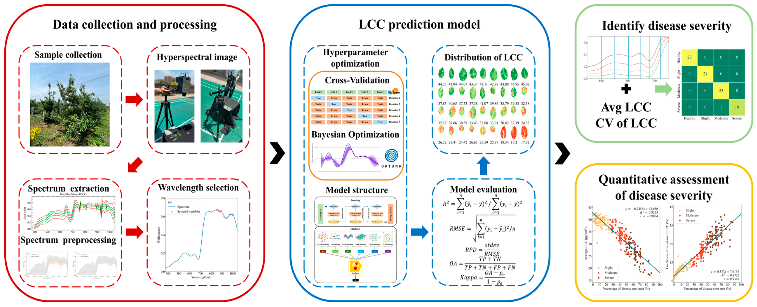
2. Materials and Methods

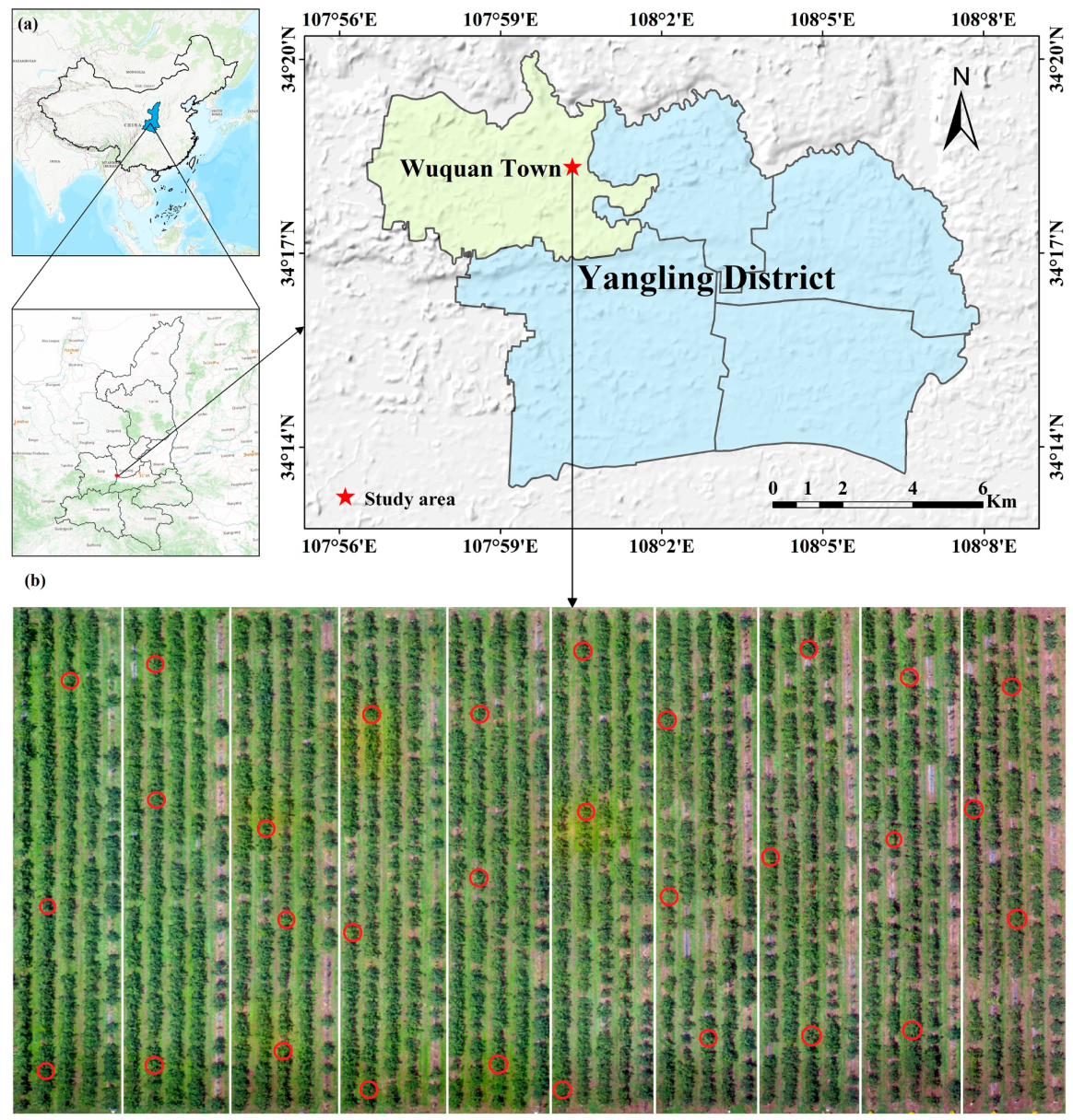
2.1. Leaf Sample Collection

Data collection was conducted on 23 July 2022 at an orchard in Wuquan Town, Yangling District, Xianyang City, Shaanxi Province (108.010969°E, 34.30475°N). Thus, 30 apple trees were selected, from which 3 healthy and 9 infected leaves were collected from each tree via visual inspection according to the rules in

Table 1. Degree of leaf disease and measurement area.

Disease Severity	Percentage of Disease Spot Area	Number of Measurements	Measurement Area
health	0%	2	Two random uninfected areas
slight	0~25%	3	Two random uninfected areas and one infected area
moderate	25~50%	3	One random uninfected area and two infected areas
severe	>50%	2	Two random infected areas

(360 leaves in total). All trees were ten-years-old, grown under the same irrigation and fertilization conditions, and infected only with ApMV. The location of the study area and sampled trees is shown in Figure 1. All collected leaves were sealed in plastic bags and stored in a thermos with ice packs to maintain their freshness for transport to the laboratory.

2.2. Data Acquisition

2.2.1. LCC Determination

The Dualex 4, an optical leaf analyzer developed by Force-A (Orsay, France), is capable of accurate and non-destructive determination of LCC in real time [34]. The analyzer used in this study can measure leaf chlorophyll content (LCC) within 1 s. The measurement results are numerical values in μg/cm², which are stored in the analyzer, and the data can be transferred to a personal computer via a USB cable. Following the rules outlined in Table 1, the corresponding areas on all leaves were selected for measurement, and the average of the measured values was taken as the chlorophyll content value of that leaf. In this way, a total of 360 leaf chlorophyll content values were obtained.

2.2.2. Hyperspectral Image Acquisition

An SOC 710VP portable hyperspectral imager (Surface Optics Corp., San Diego, CA, USA) was used to acquire hyperspectral images using built-in push-sweep spectral imaging technology. This allowed for quick, convenient, and accurate acquisition of HSI in the field. The system had a spectral range and resolution of 374.81–1042.15 nm and 4.6875 nm, respectively, with 128 bands and an imaging resolution of 696 × 520. The hyperspectral imaging system included SOC 710VP, a standard gray panel, low-reflectivity black cotton cloth, and a tripod. It was set up on the rooftop of the College of Resources and Environment, Northwest A&F University, in an outdoor area with sunlight and no shadows. HSIs were obtained under clear, windless weather conditions from 10:00 to 14:00 on 23 July 2022. Each leaf was placed horizontally on a black cotton cloth with a standard gray panel, and HSIs were taken with the system pointing vertically downward onto the leaves after focusing to obtain a clear image. The acquired hyperspectral images were calibrated using SRAnalysis™ Version 3.0 software with the following calibration equation:

$$R_{\lambda }=\frac{I_{\lambda }-D_{\lambda }}{W_{\lambda }-D_{\lambda }},$$

(1)

where $R_{\lambda }$ is the corrected image, $I_{\lambda }$ is the original image, $D_{\lambda }$ is the dark current image, and $W_{\lambda }$ is the reference plate image. Using the region of interest tool in ENVI 5.3 (Research System Inc., Boulder, CO, USA), the average spectral reflectance of the chlorophyll measurement location was extracted from the calibrated leaf image as the spectral data of the leaf. A total of 360 spectral samples were obtained. The spectral reflectance of the leaf and background in the hyperspectral image showed the greatest difference at 701.38 nm. Thus, the binarized image at 701.38 nm was obtained via segmentation with a threshold of 0.25 in MATLAB R2021b (MathWorks, Natick, MA, USA) to remove the background. Similarly, the binarized image at 649.05 nm was segmented with a threshold of 0.15 to separate the disease spots and calculate their areas.

2.3. Data Processing

To quantitatively assess the disease severity based on LCC, we established a method to invert the LCC distribution of leaves based on HSI (Figure 2). First, we measured LCC and calculated the percentage of diseased spot area using the threshold segmentation method. Next, we preprocessed the extracted spectral reflectance to reduce the effect of environmental noise and selected the optimal wavelength combination using the competitive adaptive reweighted sampling (CARS) algorithm. Additionally, we established a high-performance Stacked–Boosting prediction model of LCC based on a Stacking and Boosting ensemble learning strategy. We mapped the LCC distribution using the model and calculated the average LCC for each leaf to analyze the correlation between LCC and disease severity. Finally, we combined the average LCC with sensitive wavelengths for disease severity identification.

2.3.1. Spectral Data Pre-Processing

External environmental factors during the spectral data acquisition can generate random noise that affects prediction accuracy. Pre-processing spectral data is essential to reduce the impact of external factors to some extent. Therefore, we used the Savitzky–Golay (SG) algorithm to filter and denoise the raw spectral data. The SG algorithm effectively reduces the random noise in the spectral data, improving the data’s accuracy without distorting the signal’s trend [35]. In this study, quadratic polynomial 15-point smoothing was selected for noise reduction in the spectral data, as it had a good noise reduction effect. Figure 3 shows the original spectral reflectance curve and the SG-filtered spectral reflectance curve. The original spectral reflectance curve was noisy in the visible range greater than 750 nm and the near-infrared spectrum. In contrast, the SG-filtered spectral reflectance curve effectively reduced the noise without changing the spectral reflectance curve’s trend.

2.3.2. Sample Split

Different sample split algorithms can lead to varying results. Prior to building the model, we used the SPXY algorithm to split all 360 spectral samples into calibration (270 samples) and validation (90 samples) sets at a 3:1 ratio for calibrating and validating the model, respectively. The SPXY algorithm was developed from the Kennard–Stone algorithm, which considers all samples as candidates, selects the two samples with the farthest sample distance, and then puts these two samples in the calibration set in turn until reaching the set ratio. The SPXY method considers both the features and labels of the samples when calculating the sample distances, ensuring that the samples in the calibration set are evenly distributed according to the spatial distances. This approach effectively covers the multidimensional vector space, improving the prediction ability of the proposed model [36,37].

Table 2. Basic characteristics of the sample.

Sample	Number of Samples	Minimum (μg/cm2)	Maximum (μg/cm2)	Mean (μg/cm2)	Standard Deviation
Calibration set	270	4.14	55.60	28.93	13.27
Validation set	90	6.30	53.62	35.42	13.21
Total	360	4.14	55.60	30.55	13.53

shows the dataset split using the SPXY algorithm.

2.3.3. Feature Selection Method

Hyperspectral data contain a significant amount of redundant information that can affect the model’s performance and prediction accuracy. In this study, we utilized the CARS algorithm, an iterative statistical information-based variable selection algorithm based on the Darwinian principle of “survival of the fittest”, to select characteristic wavelengths. This method combines a partial least squares regression model using an adaptive weighted sampling technique and exponential decay function to retain wavelengths with larger absolute values of regression coefficients and remove features with smaller absolute values of regression coefficients in the partial least squares regression model. It uses cross-checking to filter the subset of variables with the smallest root mean square error in cross-validation (RMSECV) as the optimal subset of variables [38,39]. We implemented the CARS algorithm through the LibPLS v1.98 toolbox [40].

2.3.4. Spectral Sensitivity Index

Spectral sensitivity index (SI) can be used to express the difference in spectral reflectance between different leaves. The SI is calculated as follows:

$$SI=\frac{R_D-R_H}{R_H}$$

(2)

where $R_D$ is the spectral reflectance of leaves infected with ApMV, and $R_H$ is the average spectral reflectance of the healthy leaves. Equation (2) shows that when $SI>0$, the spectral reflectance of diseased leaves is higher than healthy leaves at a certain wavelength. As SI increases, the difference in spectral reflectance between diseased leaves and healthy leaves is more significant and vice versa. Using $SI$ to analyze sensitive wavelengths for disease monitoring partially eliminates the influence of environmental noise on the spectra, making the spectra of different disease severities more comparable, thus improving the accuracy of monitoring [41].

2.3.5. Coefficient of Variation

The coefficient of variation ($CV$) is the ratio of the standard deviation of the data to the average value. $CV$ can eliminate the effect of average and compare the degree of variation among different samples. The $CV$ is calculated as follows:

$$CV=\frac{\sigma }{\mu }\times 100\%$$

(3)

where $\sigma$ is the standard deviation of the sample, and $\mu$ is the the average of the sample. Data variability is low when $CV$ < 15, medium when 15 < $CV$ < 35, and high when $CV$ > 35 [42]. $CV$ can be used to express the complexity in LCC distribution, which reflects the degree of dispersion of LCC distribution.

2.4. Modeling Method

2.4.1. Basic Models

In this study, seven machine learning models were selected as the base learners of Stacked–Boosting models: classification and regression tree (CART), elastic network (EN), Gaussian process regression (GPR), K-nearest neighbor regression (KNN), kernel ridge regression (KRR), multilayer perceptron (MLP), and support vector machine regression (SVR). Classification and regression tree (CART) is a prediction model that predicts the value of an outcome variable based on other values. It partitions predictor variables into branches, with each end node containing a prediction of the outcome variable. CART is easy to understand and interpret, requires little data preparation, and handles large-scale data very well [43,44]. The Elastic Network (EN) is a regularized regression method that linearly combines the L1 penalty of the lasso method and the L2 penalty of the ridge method [45]. It adds a regularization term to the loss function for fast training and has simple parameters that prevent overfitting [46]. Gaussian Process Regression (GPR) is a nonparametric Bayesian regression method that infers the probability distribution of all possible values without being restricted by functional form [47]. GPR works well on small datasets and provides predictive uncertainty measures. K-nearest neighbor algorithm (KNN) is a simple, nonparametric supervised learning classifier that uses proximity to make predictions for groupings of individual data points, making it sensitive to the local structure of the data [48]. In regression problems, KNN uses the average of K-nearest neighbors to predict continuous values. Ridge regression is a method for estimating coefficients of a multiple regression model with highly correlated independent variables [45]. kernel ridge regression (KRR) combines ridge regression with the kernel technique to learn linear functions in the space induced by the corresponding kernel and data [49]. Multilayer perceptron (MLP) is an artificial neural network that maps input vectors to output vectors. It overcomes the limitation of perceptron by recognizing linearly indistinguishable data [50]. Support vector machine regression (SVR) uses support vectors from training samples to design optimal decision boundaries. It is a nonlinear modeling method based on statistical learning theory and can solve both linear and nonlinear regression modeling problems [51,52].

2.4.2. Stacked–Boosting for Predictive Models

Stacking is an ensemble learning strategy, which fuses multiple models and typically consists of two levels: level 0 with two or more base learners, and level 1 with a meta-learner that combines the predicted values of base learners. The predicted values of each base learner (Figure 4, P₁–P₆) are used as input features for the meta-learner [53,54]. At level 0, algorithms with significant differences, in principle, are usually chosen as base learners and cross-validated to train the models. At level 1, a model with better predictive performance, stable performance, and strong generalization ability is typically selected as a meta-model to incorporate the predictions from the base models. Compared to a single machine learning model, Stacking models can combine the advantages of multiple algorithms and exhibit stronger predictive and generalization capabilities [53].

Boosting is an ensemble learning strategy that can transform weak learners into strong ones to improve the predictive performance of machine learning algorithms [54,55]. AdaBoost is a representative algorithm for Boosting integrated learning [56,57]. The core idea of this algorithm is to modify the weight of each sample based on its regression prediction error, pass the modified weights to the next learner for training, focus more on poorly performing samples in the previous iteration of learning, and finally fuse the weak learners obtained from each training stage into a strong learner. The weighted average of the predictions is used as the final output, meaning the AdaBoost algorithm can effectively improve the prediction accuracy of the base learner with less overfitting [53,58]. The traditional AdaBoost algorithm usually uses CART as the base learner. In this study, seven machine learning models were used as the base learners of AdaBoost to achieve the Boosting ensemble of different models: classification and regression tree (CART), elastic network (EN), Gaussian process regression (GPR), K-nearest neighbor regression (KNN), kernel ridge regression (KRR), multilayer perceptron (MLP), and support vector machine regression (SVR). These seven models differ significantly in principle, and the better-performing model can be selected as the base learner of the Stacking model.

CatBoost is a decision-tree-based gradient-boosting machine learning method that uses a symmetric decision tree as the base learner. This method employs ranking boosting to combat noisy points in the calibration set, thus reducing the need for much hyperparameter tuning, reducing the possibility of overfitting, improving the model generalizability, avoiding bias in gradient estimation, and solving the problem of prediction bias, all of which improve the model’s predictive and generalization capabilities [59,60]. Therefore, the CatBoost model was selected as the meta-learner for the Stacking model in this study (Figure 4).

To maximize the use of limited samples and improve the prediction accuracy and training efficiency, we used 5-fold cross-validation and Bayesian optimization to determine the hyperparameters of each model, which were implemented with the Scikit-learn library [61] and Optuna library [62], respectively. The search range of hyperparameters for each model is shown in

Table 3. Hyperparameter tuning range.

Models	Hyperparameters and the Search Range
CART	max_depth: (2~20)
EN	alpha: (0.01~10), L1_ratio: (0~1)
GPR	alpha: (1 × 10−10), n_restarts_optimizer: (1~50)
KNN	weight: distance, n_neighbors: (1~10), p: (1~10)
KRR	kernel: laplacian, alpha: (0.01~1)
MLP	solver: lbfgs, hidden_layer_sizes: (0~100,0~100), learning_rate: (0.01~1)
SVR	kernel: rbf, C: (1~10), gamma: (0.5~5)
AdaBoost	base_estimator: (CART, EN, GPR, KRR, MLP, SVR), n_estimators: (1~100), learning_rate: (0.01~1)
CatBoost	task_type: GPU, iterations: (10~500), depth: (2~10), learning_rate: (0.01~1), L2_leaf_reg: (1~50)

.

2.4.3. Model Evaluation Methodology

To evaluate the prediction accuracy and generalization ability of different models, the coefficient of determination ($R^2$), root mean square error ($RMSE$), and residual predictive deviation ($RPD$) were calculated using the following formulas:

$$R^2={\displaystyle \sum }_{i=1}^n{\left({\widehat{y}}_i-\overline{y}\right)}^2/{\displaystyle \sum }_{i=1}^n{\left(y_i-\overline{y}\right)}^2$$

(4)

$$RMSE=\sqrt{{\displaystyle \sum }_{i=1}^n{\left(y_i-{\widehat{y}}_i\right)}^2/n}$$

(5)

$$RPD=\frac{stdev}{RMSE}$$

(6)

where $y_i$ is the measured value, $\overline{y}$ is the average of the measured values, ${\widehat{y}}_i$ is the predicted value, $n$ is the number of samples, and $stdev$ is the standard deviation. The closer the $R^2$ value is to 1, the smaller the $RMSE$ and the higher the prediction accuracy of the model; $RPD$ greater than 2 indicates very good model prediction ability, $RPD$ between 1.4 and 2 indicates average model prediction ability, and $RPD$ less than 1.4 indicates poor predictive power in the model [63].

Overall accuracy (OA) and Kappa coefficients were used to assess the accuracy of identification of disease severity. The specific formulas for OA and Kappa were calculated as follows:

$$OA=\frac{TP+TN}{TP+TN+FP+FN}$$

(7)

$$Kappa=\frac{OA-p_e}{1-p_e}$$

(8)

$$p_e={\displaystyle \sum }_{i=1}^C\frac{T{P}_i+F{N}_i+T{P}_i+F{P}_i}{N^2}$$

(9)

where $TP$ is true positives, $TN$ is true negatives, $FP$ is false positives, $FN$ is t false negatives, $C$ is the number of classes, and $N$ is the number of samples. The closer the OA value is to 100% and the closer the Kappa coefficients are to 1, the higher the classification accuracy of the model.

3. Results

3.1. Spectral Characteristics of Leaves

The spectral characteristics of plants are influenced by their internal structure, biochemical composition, and morphological features [31], and the cells of leaves infected with ApMV are damaged, with irregular yellowish- to cream-colored spots, decreased chlorophyll content, and differences in spectral reflectance. Significant differences in spectral reflectance and SI were observed for regions with differing LCC (Figure 5). The spectral curves of the healthy regions with an LCC of 45.66 μg/cm² had weak reflection peaks in the green band at 550 nm and two absorption valleys in the blue band at 450 nm and the red band at 680 nm, which were consistent with the reflectance spectral characteristics of green plants. However, as disease severity increases and LCC decreases, two prominent reflection peaks appeared in the green band at 550 nm and the red band at 650 nm, while the red edge (680–730 nm) shifted toward the short-wave direction. The large SI values were concentrated in the visible spectrum range (380–750 nm), indicating that the differences in leaf spectral reflectance in the visible band under different disease severities were significant, and the leaf spectral reflectance increased gradually with increasing disease severity. In the near-infrared spectrum range (750–1100 nm), the differences in spectral reflectance in regions with different LCC were relatively small, and the SI was almost 0 for different disease severities. This was due to the influence of internal structure, biochemical composition, and morphological features of the plant on its spectral characteristics [31]. ApMV damages the structure of mesophyll tissues, resulting in reduced photosynthetic capacity and, thus, reduced absorption of red and blue bands, which consequently results in a significant increase in spectral reflectance in the visible spectrum range (380–750 nm).

3.2. Characteristic Wavelength Extraction

The raw spectral reflectance data were smoothed using the SG algorithm and used as input data. The number of iterations for the CARS algorithm was determined based on the minimum RMSECV in the PLSR model. Figure 6 shows the results of 50 iterations of the CARS algorithm and the selected optimal wavelength combination locations. As the CARS algorithm iterated and the number of selected wavelengths decreased, the RMSECV value first decreased and then increased. The lowest RMSECV value was found in the 26th iteration, indicating that wavelengths that were poorly correlated with LCC were eliminated in the 1st to 26th iterations. The iterations after the 26th may have eliminated wavelengths more strongly correlated with LCC, leading to a decrease in model accuracy and an increase in RMSECV. Therefore, we used the wavelength combination selected in the 26th iteration of the CARS algorithm for modeling and validation. We finally selected 15 feature wavelengths, mainly concentrated in the red-edge position and near-infrared range: 701.38 nm, 717.17 nm, 727.72 nm, 850.47 nm, 855.86 nm, 861.26 nm, 872.07 nm, 882.91 nm, 893.76 nm, 899.19 nm, 920.97 nm, 948.31 nm, 959.27 nm, 992.29 nm, and 1003.3 nm, as shown in Figure 6d. These constitute only 12% of the original wavelengths (128), demonstrating that the CARS algorithm can effectively reduce modeling complexity [32].

3.3. Modeling Evaluation of LCC Prediction

The 15 feature wavelengths selected by the CARS algorithm were used as the model’s input data. Seven models, classification and regression tree (CART), elastic network (EN), Gaussian process regression (GPR), K-nearest neighbor regression (KNN), kernel ridge regression (KRR), multilayer perceptron (MLP), and support vector machine regression (SVR), were used to make predictions. These seven models were used as the base learners for AdaBoost for Boosting ensemble to construct predictive models. Finally, Stacked–Boosting prediction models were constructed. The results are shown in

Table 4. Modeling results.

Model	${\mathit{R}\mathit{M}\mathit{S}\mathit{E}}_{\mathit{c}}$	${\mathit{R}}_{\mathit{c}}^2$	${\mathit{R}\mathit{M}\mathit{S}\mathit{E}}_{\mathit{v}}$	${\mathit{R}}_{\mathit{v}}^2$	$\mathit{R}\mathit{P}\mathit{D}$
CART	3.8288	0.9164	4.6980	0.8722	2.6818
EN	3.0413	0.9473	3.4346	0.9317	3.3022
GPR	2.1294	0.9741	3.8393	0.9146	3.3059
KNN	0.0000	1.0000	3.3096	0.9367	3.9322
KRR	2.1399	0.9739	3.0436	0.9463	4.0729
MLP	3.0368	0.9474	3.2271	0.9397	4.1084
SVR	2.7234	0.9577	3.4373	0.9316	3.4026
CART-Boosting	2.4479	0.9658	2.7598	0.9559	4.7031
EN-Boosting	3.0095	0.9484	3.3658	0.9344	3.3512
GPR-Boosting	1.4083	0.9887	3.1167	0.9437	4.1014
KNN-Boosting	0.0493	1.0000	3.0414	0.9404	4.3078
KRR-Boosting	2.0279	0.9765	2.9451	0.9498	4.2451
MLP-Boosting	2.5351	0.9634	2.7623	0.9558	4.7044
SVR-Boosting	2.6465	0.9601	3.3853	0.9336	3.4364
Stacked-Boosting	1.3608	0.9894	2.4796	0.9644	5.1054

.

Among the models, the KNN model and KNN-Boosting model had an $R_c^2$ of 1. However, the prediction accuracy of the validation set was low, indicating that it shows severe overfitting. Therefore, KNN-Boosting was not used as the base model for the Stacking model. The prediction accuracy of the KRR model was the highest among the seven base models, with $R_c^2$ and $R_v^2$ of 0.9739 and 0.9463, respectively, and the $RPD$ value was 4.0729. The CART model had a poorer prediction accuracy among the seven base models, with an $R_v^2$ of 0.8722, relatively high $RMS{E}_v$, and $RPD$ of only 2.6818. The prediction accuracy of all seven base models improved after Boosting ensemble, among which the CART-Boosting model showed the most noticeable performance improvement, with $R_c^2$ increasing by 0.0494, $R_v^2$ increasing by 0.0837, and $RPD$ increasing by 2.0213. This was followed by the MLP-Boosting model, whose $R_v^2$ reached 0.9558. In comparison, the Stacked–Boosting model performed the best, with $R_c^2$ of 0.9894, $R_v^2$ of 0.9644, and $RPD$ of 5.1054. The difference in the coefficient of determination between the calibration and validation sets was slight. The $RMS{E}_v$ was only 2.4796 μg/cm², indicating that the Stacked–Boosting model had higher prediction accuracy and strong generalization ability.

3.4. Inversion of LCC by HSI

In this study, we monitored the LCC distribution of leaves with different disease se-verity and used the characteristic wavelengths as the input data for the Stacked–Boosting model to calculate the average LCC by inversing the LCC distribution. Figure 7 shows the RGB images and LCC distribution of leaves with varying disease severity and their average LCC. The RGB images show that the healthy areas of the leaves were dark green. On the lightly infected leaves, the diseased spots were light yellow and showed diseased spots and streaks along the veins. On the most severely infected leaves, the diseased spots were creamy white and showed a reticulated distribution, uninfected areas appeared light green, while the uninfected areas of the other leaves appeared dark green. This result indicates that the cell structure of the leaf area infected with ApMV was damaged, which reduced the LCC and affected the uninfected area. The LCC distribution image and the average LCC also confirmed this phenomenon. In the infected area, the LCC decreased from the periphery to the center of the diseased spot. In the uninfected area, the LCC of the area near the diseased spot was lower than that of the area far from the diseased spot, indicating that the uninfected area will be affected by the infected area because the infected area has a tendency to expand. Visual comparison showed that the inversion of LCC distribution using the Stacked–Boosting model was consistent with the actual distribution trend. The average LCC decreased with increasing disease area, which was consistent with the fact. This indicates that the model was reliable.

3.5. Relationship between LCC Statistics and Percentage of Disease Spot Area

The LCC distribution allowed for the computation of the average and CV of LCC for each leaf. Figure 8 depicts the relationship between these two LCC statistics and the percentage of disease area. As illustrated in Figure 8, there was a highly significant negative correlation between the average LCC and the percentage of the diseased area (r = −0.9084), while the CV of LCC was positively correlated with the percentage of diseased area (r = 0.9314) [64]. The increase in the percentage of disease area resulted in a gradual decrease in the average LCC and an increase in the CV of LCC. This trend can be attributed to the uneven LCC distribution resulting from increased disease severity and reduced LCC in infected areas. Therefore, changes in LCC offer a quantitative indicator for monitoring disease severity on ApMV-infected leaves.

3.6. Identify Disease Severity Based on Average LCC and Sensitive Wavelengths

In Section 3.1, we found that the spectral reflectance of leaves with different levels of disease severity differed the most in the visible spectrum range, making it useful for distinguishing among different levels of disease. As shown in Figure 5a, regions of large differences in reflectance in the visible spectrum range are located at reflection peaks of 550.95 nm and 649.05 nm and absorption valleys of 602.36 nm and 680.39 nm. As shown in Figure 5b, the SI at 500.02 nm is significantly higher than that at adjacent wavelengths, indicating large differences in reflectance among leaves with different levels of disease at this wavelength. These wavelengths are more sensitive to disease severity, which can effectively reflect the features of leaves with different levels of disease and are helpful for distinguishing among different levels of disease [18]. The red edge region of plants (680–730 nm) is significantly correlated to LCC and can effectively monitor changes in LCC, making it a useful indicator of plant vitality [65]. Therefore, the wavelength of 722.44 nm can also be used to distinguish among different levels of disease [66]. Additionally, the average LCC is highly correlated with disease severity and can be used as a feature to distinguish between different levels of disease. In summary, we selected six sensitive wavelengths (500.02 nm, 550.95 nm, 602.36 nm, 649.05 nm, 680.39 nm, and 701.38 nm) and the average LCC as features to distinguish among different levels of disease.

Table 5. Identification modeling results.

Feature	$\mathit{O}{\mathit{A}}_{\mathit{c}}/\mathit{\%}$	${\mathit{K}\mathit{a}\mathit{p}\mathit{p}\mathit{a}}_{\mathit{c}}$	$\mathit{O}{\mathit{A}}_{\mathit{v}}/\mathit{\%}$	${\mathit{K}\mathit{a}\mathit{p}\mathit{p}\mathit{a}}_{\mathit{v}}$
500.02 nm	97.04	0.9604	74.44	0.6573
550.95 nm	93.70	0.9161	86.67	0.8188
602.36 nm	96.67	0.9556	85.56	0.8045
649.05 nm	97.04	0.9604	78.89	0.7150
680.39 nm	93.70	0.9159	66.67	0.5550
722.44 nm	90.37	0.8713	57.78	0.4441
Average LCC	91.85	0.8913	91.11	0.8811
CV of LCC	93.33	0.9111	81.11	0.7468
all sensitive wavelengths	97.41	0.9654	92.22	0.8960
all LCC statistics	97.78	0.9704	95.56	0.9406
sensitive wavelengths + LCC statistics	99.26	0.9901	98.89	0.9852

shows the classification results of the Random Forest model based on different sensitive wavelengths, average LCC, and their combinations. Among them, the classification based on the wavelength of 550.95 nm had the best accuracy among the single wavelengths, with an $O{A}_v$ of 86.67% and $Kapp{a}_v$ of 0.8188. The accuracy of classification based on all sensitive wavelengths was higher than that based on a single wavelength, with an $O{A}_v$ of 92.22% and $Kapp{a}_v$ of 0.8960. The classification accuracy based on all LCC statistics is higher than that based on a single statistic, with an $O{A}_v$ of 95.56% and $Kapp{a}_v$ of 0.9406. The combination of all sensitive wavelengths and all LCC statistics had the highest accuracy, with an $O{A}_v$ of 98.89% and $Kapp{a}_v$ of 0.9852, and the confusion matrix of the classification results is shown in Figure 9. Yellowish color means larger value, greenish color means smaller number.

4. Discussion

4.1. Stacked–Boosting Modeling Summary

The Stacked–Boosting model exhibited the best prediction performance among all models, did not produce overfitting, and had high generalization ability. To further compare the prediction performance of the Stacked–Boosting model and the traditional ensemble learning model, a Random Forest model with a bagging strategy and XGBoost model with the gradient boosting strategy was applied to construct an LCC prediction model using the same dataset. The accuracy and prediction scatter plots of the models are shown in Figure 10. The overall prediction accuracy of the Random Forest model was lower than that of the Stacked–Boosting model, and it exhibited significant deviation between the predicted and measured values. The XGBoost model was overfitted; it had high prediction accuracy in the calibration set but lower prediction accuracy in the validation set than that of the Stacked–Boosting model. When compared with prediction values of the traditional ensemble learning model, the Stacked–Boosting model had a more concentrated distribution around the 1:1 line (Figure 9). This result indicates that the generalization ability and overall prediction performance of the Stacked–Boosting model were superior to those of the traditional integrated learning model.

The Stacked–Boosting model exhibited excellent prediction performance and generalization ability for several reasons. First, the integration strategy of Boosting improves the prediction performance of weak learners, which can indirectly improve the final prediction performance. Secondly, using significantly different base learner models for the Stacking model can leverage the advantages of each algorithm. Finally, using the CatBoost model provided better prediction performance as the meta-learners of the Stacking model could properly consider the weights of the different base learner prediction results of and reduce the errors caused by poorly performing base learners.

As the meta-learners of the Stacking model directly use the prediction results of the base learners as input data, the selection of the base learners directly affects the final prediction accuracy. As shown in Figure 11, the importance of different feature variables varies widely, and, thus, the importance of the prediction results from the different base learners on the final prediction also varies widely. Therefore, in practice, when selecting the most appropriate to improve prediction performance and reduce computational overhead, the characteristics of the base learners and their degree of importance to the final prediction should be considered.

4.2. Quantitative Description of Disease Severity Using Chlorophyll Content

Diseased spot color, morphology, and affected area percentage have typically been used as criteria for grading disease severity [23,27,67]. However, these methods fail to consider the role of phytochemical components, making it difficult to obtain objective and accurate grading results. The LCC of plants is influenced by factors, such as temperature, water, and light, and aging can also lead to a decrease in LCC [68,69,70,71]. However, in this experiment, the leaves were collected under the same environmental conditions, and ApMV was found to be the most important factor causing significant changes in LCC. As shown in the LCC distribution in Figure 7, the impact of ApMV on LCC was extremely significant. At all levels of disease severity, the LCC of diseased areas was always lower than that of healthy regions, and the average LCC of severely infected leaves was even lower. This study also found a strong correlation between LCC and disease severity. Using LCC as a feature could improve the accuracy of identifying disease severity, and good identification accuracy ($O{A}_v$ = 95.56) was obtained using only two LCC statistics. These findings suggest that LCC can serve as a quantitative indicator to assess the severity of ApMV infection.

5. Conclusions

An LCC prediction model and a disease severity identification model were developed based on the HSI of ApMV-infected apple leaves to verify the feasibility of using HSI to identify ApMV infection and quantitatively describe the leaf health condition. The results demonstrated that the Stacked–Boosting model had higher prediction accuracy and generalization ability than the traditional ensemble learning model and could be used to invert the LCC. The average LCC was obtained from the LCC distribution images and could be used for a quantitative description of leaf health and photosynthetic capacity. It can also be used for identifying disease severity. This method considered the role of phytochemical components, which is more accurate than using the disease area as the only indicator of disease extent. However, model construction, hyperparameter optimization, and computational overhead are highly complex. Therefore, subsequent studies should give more consideration to the type and number of base learners to explore ways to reduce the model complexity. Our proposed method can also be used to assess plant leaf health under other biotic or physicochemical stresses. Nonetheless, it is important to note that LCC is influenced by several factors, and our study only applied to leaves known to be infected with ApMV. For unknown leaves, LCC alone may not be sufficient to determine whether they are infected with ApMV. Therefore, an early monitoring method for identifying ApMV infection should be explored in future studies. Furthermore, this study only achieved a quantitative description of disease severity at the leaf scale, and the health status of the entire apple tree was not assessed. Future research should explore the application of our method as a preliminary step in the development of a more comprehensive canopy-scale tree health assessment method.

References

1. Grimova, L.; Winkowska, L.; Konrady, M.; Rysanek, P. Apple mosaic virus. Phytopathol. Mediterr. 2016, 55, 1–19. [Google Scholar]
2. Dursunoglu, S.; Ertunc, F. Distribution of Apple Mosaic Ilarvirus (ApMV) in Turkey. Acta Hortic. 2008, 781, 131–134. [Google Scholar]
3. Chen, T.; Zeng, R.; Guo, W.; Hou, X.; Lan, Y.; Zhang, L. Detection of Stress in Cotton (Gossypium hirsutum L.) Caused by Aphids Using Leaf Level Hyperspectral Measurements. Sensors 2018, 18, 2798. [Google Scholar] [CrossRef] [PubMed]
4. Un Nabi, S.; Yadav, M.; Yousuf, N.; Raja, W.; Sidharthan, K.; Dubey, S.; Kumar, M.; Jaiswal, D. Apple Mosaic Disease: Potential Threat to Apple Productivity. EC Agric. 2019, 5, 614–618. [Google Scholar]
5. Gitelson, A.A.; Merzlyak, M.N. Remote estimation of chlorophyll content in higher plant leaves. Int. J. Remote Sens. 1997, 18, 2691–2697. [Google Scholar] [CrossRef]
6. Moustakas, M.; Calatayud, Á.; Guidi, L. Chlorophyll fluorescence imaging analysis in biotic and abiotic stress. Front. Plant Sci. 2021, 12, 658500. [Google Scholar] [CrossRef]
7. Jiang, X.; Zhen, J.; Miao, J.; Zhao, D.; Shen, Z.; Jiang, J.; Gao, C.; Wu, G.; Wang, J. Newly-developed three-band hyperspectral vegetation index for estimating leaf relative chlorophyll content of mangrove under different severities of pest and disease. Ecol. Indic. 2022, 140, 108978. [Google Scholar] [CrossRef]
8. Peng, Y.; Nguy-Robertson, A.; Arkebauer, T.; Gitelson, A.A. Assessment of Canopy Chlorophyll Content Retrieval in Maize and Soybean: Implications of Hysteresis on the Development of Generic Algorithms. Remote Sens. 2017, 9, 226. [Google Scholar] [CrossRef]
9. Merzlyak, M.N.; Gitelson, A.A.; Chivkunova, O.B.; Rakitin, V.Y. Non-destructive optical detection of pigment changes during leaf senescence and fruit ripening. Physiol. Plant. 1999, 106, 135–141. [Google Scholar] [CrossRef]
10. Tian, M.L.; Ban, S.T.; Chang, Q.R.; Zhang, Z.R.; Xu-Mei, W.U.; Wang, Q. Quantified Estimation of Anthocyanin Content in Mosaic Virus Infected Apple Leaves Based on Hyperspectral Imaging. Spectrosc. Spectr. Anal. 2017, 37, 3187–3192. [Google Scholar]
11. Ban, S.; Tian, M.; Chang, Q. Estimating the severity of apple mosaic disease with hyperspectral images. Int. J. Agric. Biol. Eng. 2019, 12, 148–153. [Google Scholar] [CrossRef]
12. Medina-Puche, L.; Lozano-Duran, R. Tailoring the cell: A glimpse of how plant viruses manipulate their hosts. Curr. Opin. Plant Biol. 2019, 52, 164–173. [Google Scholar] [CrossRef]
13. Liu, Y.; Zhou, S.; Wu, H.; Han, W.; Li, C.; Chen, H. Joint optimization of autoencoder and Self-Supervised Classifier: Anomaly detection of strawberries using hyperspectral imaging. Comput. Electron. Agric. 2022, 198, 107007. [Google Scholar] [CrossRef]
14. Lowe, A.; Harrison, N.; French, A.P. Hyperspectral image analysis techniques for the detection and classification of the early onset of plant disease and stress. Plant Methods 2017, 13, 80. [Google Scholar] [CrossRef]
15. Cui, B.; Ye, H.; Liu, L.; Wu, M.; Huang, W.; Dong, Y.; Shi, Y. Progress and prospects of crop diseases and pests monitoring by remote sensing. Smart Agric. 2019, 1, 1. [Google Scholar] [CrossRef]
16. Zhang, N.; Yang, G.; Zhao, C.; Zhang, J.; Yang, X.; Pan, Y.; Huang, W.; Xu, B.; Li, M.; Zhu, X. Progress and prospects of hyperspectral remote sensing technology for crop diseases and pests. Natl. Remote Sens. Bull. 2021, 25, 403–422. [Google Scholar]
17. Liu, F.; Xiao, Z. Disease spots identification of potato leaves in hyperspectral based on locally adaptive 1D-CNN. In Proceedings of the 2020 IEEE International Conference on Artificial Intelligence and Computer Applications (ICAICA), Dalian, China, 27–29 June 2020; pp. 355–358. [Google Scholar]
18. Wei, X.; Johnson, M.A.; Langston, D.B.; Mehl, H.L.; Li, S. Identifying Optimal Wavelengths as Disease Signatures Using Hyperspectral Sensor and Machine Learning. Remote Sens. 2021, 13, 2833. [Google Scholar] [CrossRef]
19. Abdulridha, J.; Batuman, O.; Ampatzidis, Y. UAV-Based Remote Sensing Technique to Detect Citrus Canker Disease Utilizing Hyperspectral Imaging and Machine Learning. Remote Sens. 2019, 11, 1373. [Google Scholar] [CrossRef]
20. Khan, I.H.; Liu, H.; Li, W.; Cao, A.; Wang, X.; Liu, H.; Cheng, T.; Tian, Y.; Zhu, Y.; Cao, W.; et al. Early Detection of Powdery Mildew Disease and Accurate Quantification of Its Severity Using Hyperspectral Images in Wheat. Remote Sens. 2021, 13, 3612. [Google Scholar]
21. Guo, A.; Huang, W.; Dong, Y.; Ye, H.; Ma, H.; Liu, B.; Wu, W.; Ren, Y.; Ruan, C.; Geng, Y. Wheat Yellow Rust Detection Using UAV-Based Hyperspectral Technology. Remote Sens. 2021, 13, 123. [Google Scholar] [CrossRef]
22. Gao, Z.; Khot, L.R.; Naidu, R.A.; Zhang, Q. Early detection of grapevine leafroll disease in a red-berried wine grape cultivar using hyperspectral imaging. Comput. Electron. Agric. 2020, 179, 105807. [Google Scholar] [CrossRef]
23. Bock, C.; Poole, G.; Parker, P.; Gottwald, T. Plant disease severity estimated visually, by digital photography and image analysis, and by hyperspectral imaging. Crit. Rev. Plant Sci. 2010, 29, 59–107. [Google Scholar]
24. Singhal, G.; Bansod, B.; Mathew, L.; Goswami, J.; Choudhury, B.; Raju, P. Chlorophyll estimation using multi-spectral unmanned aerial system based on machine learning techniques. Remote Sens. Appl. Soc. Environ. 2019, 15, 100235. [Google Scholar]
25. Sudu, B.; Rong, G.; Guga, S.; Li, K.; Zhi, F.; Guo, Y.; Zhang, J.; Bao, Y. Retrieving SPAD Values of Summer Maize Using UAV Hyperspectral Data Based on Multiple Machine Learning Algorithm. Remote Sens. 2022, 14, 5407. [Google Scholar] [CrossRef]
26. Gutierrez, S.; Diago, M.; Fernandez-Novales, J.; Tardaguila, J. Hyperspectral imaging application under field conditions: Assessment of the spatio-temporal variability of grape composition within a vineyard. In Precision Agriculture’19; Wageningen Academic Publishers: Wageningen, The Netherlands, 2019; pp. 811–817. [Google Scholar]
27. Luo, L.; Chang, Q.; Gao, Y.; Jiang, D.; Li, F. Combining Different Transformations of Ground Hyperspectral Data with Unmanned Aerial Vehicle (UAV) Images for Anthocyanin Estimation in Tree Peony Leaves. Remote Sens. 2022, 14, 2271. [Google Scholar]
28. Liu, N.; Wu, L.; Chen, L.; Sun, H.; Dong, Q.; Wu, J. Spectral characteristics analysis and water content detection of potato plants leaves. IFAC-PapersOnLine 2018, 51, 541–546. [Google Scholar] [CrossRef]
29. Zou, Z.; Wu, Q.; Chen, J.; Long, T.; Wang, J.; Zhou, M.; Zhao, Y.; Yu, T.; Wang, Y.; Xu, L. Rapid determination of water content in potato tubers based on hyperspectral images and machine learning algorithms. Food Sci. Technol. 2022, 42, e46522. [Google Scholar] [CrossRef]
30. Zhao, Y.-R.; Li, X.; Yu, K.-Q.; Cheng, F.; He, Y. Hyperspectral Imaging for Determining Pigment Contents in Cucumber Leaves in Response to Angular Leaf Spot Disease. Sci. Rep. 2016, 6, 27790. [Google Scholar] [CrossRef]
31. Luo, L.; Chang, Q.; Wang, Q.; Huang, Y. Identification and Severity Monitoring of Maize Dwarf Mosaic Virus Infection Based on Hyperspectral Measurements. Remote Sens. 2021, 13, 4560. [Google Scholar] [CrossRef]
32. Li, X.; Wei, Z.; Peng, F.; Liu, J.; Han, G. Estimating the distribution of chlorophyll content in CYVCV infected lemon leaf using hyperspectral imaging. Comput. Electron. Agric. 2022, 198, 107036. [Google Scholar] [CrossRef]
33. Fang, X.; Zhu, X.; Wang, Z.; Zhao, G.; Jiang, Y.; Wang, Y.a. Hyperspectral characteristics of apple leaves based on different disease stress. Remote Sens. Sci. 2014, 2, 14–21. [Google Scholar]
34. Cerovic, Z.G.; Masdoumier, G.; Ghozlen, N.B.; Latouche, G. A new optical leaf-clip meter for simultaneous non-destructive assessment of leaf chlorophyll and epidermal flavonoids. Physiol. Plant. 2012, 146, 251–260. [Google Scholar] [CrossRef]
35. Savitzky, A.; Golay, M.J. Smoothing and differentiation of data by simplified least squares procedures. Anal. Chem. 1964, 36, 1627–1639. [Google Scholar] [CrossRef]
36. Kennard, R.W.; Stone, L.A. Computer aided design of experiments. Technometrics 1969, 11, 137–148. [Google Scholar] [CrossRef]
37. Galvao, R.K.H.; Araujo, M.C.U.; José, G.E.; Pontes, M.J.C.; Silva, E.C.; Saldanha, T.C.B. A method for calibration and validation subset partitioning. Talanta 2005, 67, 736–740. [Google Scholar] [CrossRef]
38. Li, H.; Liang, Y.; Xu, Q.; Cao, D. Key wavelengths screening using competitive adaptive reweighted sampling method for multivariate calibration. Anal. Chim. Acta 2009, 648, 77–84. [Google Scholar] [CrossRef]
39. Yu, L.; Hong, Y.; Zhou, Y.; Zhu, Q.; Xu, L.; Li, J.; Nie, Y. Wavelength variable selection methods for estimation of soil organic matter content using hyperspectral technique. Trans. Chin. Soc. Agric. Eng. 2016, 32, 95–102. [Google Scholar]
40. Li, H.-D.; Xu, Q.-S.; Liang, Y.-Z. libPLS: An integrated library for partial least squares regression and linear discriminant analysis. Chemom. Intell. Lab. Syst. 2018, 176, 34–43. [Google Scholar] [CrossRef]
41. Kobayashi, T.; Kanda, E.; Kitada, K.; Ishiguro, K.; Torigoe, Y. Detection of rice panicle blast with multispectral radiometer and the potential of using airborne multispectral scanners. Phytopathology 2001, 91, 316–323. [Google Scholar] [CrossRef]
42. Zhang, J.; Jing, X.; Song, X.; Zhang, T.; Duan, W.; Su, J. Hyperspectral estimation of wheat stripe rust using fractional order differential equations and Gaussian process methods. Comput. Electron. Agric. 2023, 206, 107671. [Google Scholar] [CrossRef]
43. Quinlan, J.R. Induction of decision trees. Mach. Learn. 1986, 1, 81–106. [Google Scholar] [CrossRef]
44. Breiman, L. Classification and Regression Trees; Routledge: Abingdon-on-Thames, UK, 2017. [Google Scholar]
45. Hoerl, A.E.; Kennard, R.W. Ridge regression: Applications to nonorthogonal problems. Technometrics 1970, 12, 69–82. [Google Scholar] [CrossRef]
46. Zou, H.; Hastie, T. Regularization and variable selection via the elastic net. J. R. Stat. Soc. Ser. B (Stat. Methodol.) 2005, 67, 301–320. [Google Scholar] [CrossRef]
47. Rasmussen, C.E.; Nickisch, H. Gaussian processes for machine learning (GPML) toolbox. J. Mach. Learn. Res. 2010, 11, 3011–3015. [Google Scholar]
48. Mitchell, T.M. Machine Learning; McGraw-Hill: New York, NY, USA, 2007; Volume 1. [Google Scholar]
49. Murphy, K.P. Machine Learning: A Probabilistic Perspective; MIT Press: Cambridge, MA, USA, 2012. [Google Scholar]
50. Goodfellow, I.; Pouget-Abadie, J.; Mirza, M.; Xu, B.; Warde-Farley, D.; Ozair, S.; Courville, A.; Bengio, Y. Generative adversarial networks. Commun. ACM 2020, 63, 139–144. [Google Scholar] [CrossRef]
51. Cortes, C.; Vapnik, V. Support-vector networks. Mach. Learn. 1995, 20, 273–297. [Google Scholar] [CrossRef]
52. Chang, C.-C.; Lin, C.-J. LIBSVM: A library for support vector machines. ACM Trans. Intell. Syst. Technol. (TIST) 2011, 2, 1–27. [Google Scholar] [CrossRef]
53. Zhou, Z.-H. Ensemble Methods: Foundations and Algorithms; CRC Press: Boca Raton, FL, USA, 2012. [Google Scholar]
54. Soui, M.; Mansouri, N.; Alhamad, R.; Kessentini, M.; Ghedira, K. NSGA-II as feature selection technique and AdaBoost classifier for COVID-19 prediction using patient’s symptoms. Nonlinear Dyn. 2021, 106, 1453–1475. [Google Scholar] [CrossRef]
55. Quan, D.; Feng, W.; Dauphin, G.; Wang, X.; Huang, W.; Xing, M. A Novel Double Ensemble Algorithm for the Classification of Multi-Class Imbalanced Hyperspectral Data. Remote Sens. 2022, 14, 3765. [Google Scholar] [CrossRef]
56. Freund, Y.; Schapire, R.E. A decision-theoretic generalization of on-line learning and an application to boosting. J. Comput. Syst. Sci. 1997, 55, 119–139. [Google Scholar] [CrossRef]
57. Wu, X.; Kumar, V.; Ross Quinlan, J.; Ghosh, J.; Yang, Q.; Motoda, H.; McLachlan, G.J.; Ng, A.; Liu, B.; Yu, P.S. Top 10 algorithms in data mining. Knowl. Inf. Syst. 2008, 14, 1–37. [Google Scholar] [CrossRef]
58. Dietterich, T.G. Ensemble methods in machine learning. In Proceedings of the International Workshop on Multiple Classifier Systems, Cagliari, Italy, 21–23 June 2000; pp. 1–15. [Google Scholar]
59. Dorogush, A.V.; Ershov, V.; Gulin, A. CatBoost: Gradient boosting with categorical features support. arXiv 2018, arXiv:1810.11363. [Google Scholar]
60. Prokhorenkova, L.; Gusev, G.; Vorobev, A.; Dorogush, A.V.; Gulin, A. CatBoost: Unbiased boosting with categorical features. Adv. Neural Inf. Process. Syst. 2018, 31, 6638–6648. [Google Scholar]
61. Pedregosa, F.; Varoquaux, G.; Gramfort, A.; Michel, V.; Thirion, B.; Grisel, O.; Blondel, M.; Prettenhofer, P.; Weiss, R.; Dubourg, V. Scikit-learn: Machine learning in Python. J. Mach. Learn. Res. 2011, 12, 2825–2830. [Google Scholar]
62. Akiba, T.; Sano, S.; Yanase, T.; Ohta, T.; Koyama, M. Optuna: A next-generation hyperparameter optimization framework. In Proceedings of the 25th ACM SIGKDD International Conference on Knowledge Discovery & Data Mining, Anchorage, AK, USA, 4–8 August 2019; pp. 2623–2631. [Google Scholar]
63. Ge, Y.; Bai, G.; Stoerger, V.; Schnable, J.C. Temporal dynamics of maize plant growth, water use, and leaf water content using automated high throughput RGB and hyperspectral imaging. Comput. Electron. Agric. 2016, 127, 625–632. [Google Scholar] [CrossRef]
64. He, R.; Li, H.; Qiao, X.; Jiang, J. Using wavelet analysis of hyperspectral remote-sensing data to estimate canopy chlorophyll content of winter wheat under stripe rust stress. Int. J. Remote Sens. 2018, 39, 4059–4076. [Google Scholar] [CrossRef]
65. Zhang, Z.; Jiang, D.; Chang, Q.; Zheng, Z.; Fu, X.; Li, K.; Mo, H. Estimation of Anthocyanins in Leaves of Trees with Apple Mosaic Disease Based on Hyperspectral Data. Remote Sens. 2023, 15, 1732. [Google Scholar] [CrossRef]
66. Main, R.; Cho, M.A.; Mathieu, R.; O’Kennedy, M.M.; Ramoelo, A.; Koch, S. An investigation into robust spectral indices for leaf chlorophyll estimation. ISPRS J. Photogramm. Remote Sens. 2011, 66, 751–761. [Google Scholar] [CrossRef]
67. Wang, G.; Sun, Y.; Wang, J. Automatic image-based plant disease severity estimation using deep learning. Comput. Intell. Neurosci. 2017, 2017, 2917536. [Google Scholar] [CrossRef]
68. Alachew, E.; Muhammad, H.; Azamal, H.; Samuel, S.; Kasim, M. Differential sensitivity of Pisum sativum L. cultivars to water-deficit stress: Changes in growth, water status, chlorophyll fluorescence and gas exchange attributes. J. Agron. 2016, 15, 45–57. [Google Scholar]
69. Fu, W.; Li, P.; Wu, Y. Effects of different light intensities on chlorophyll fluorescence characteristics and yield in lettuce. Sci. Hortic. 2012, 135, 45–51. [Google Scholar] [CrossRef]
70. Bhusal, N.; Sharma, P.; Sareen, S.; Sarial, A. Mapping QTLs for chlorophyll content and chlorophyll fluorescence in wheat under heat stress. Biol. Plant. 2018, 62, 721–731. [Google Scholar] [CrossRef]
71. Wang, S.; Li, Y.; Ju, W.; Chen, B.; Chen, J.; Croft, H.; Mickler, R.A.; Yang, F. Estimation of leaf photosynthetic capacity from leaf chlorophyll content and leaf age in a subtropical evergreen coniferous plantation. J. Geophys. Res. Biogeosci. 2020, 125, e2019JG005020. [Google Scholar] [CrossRef]
Figure 1. (a) Study area. (b) Location of sampled trees.
Remotesensing 15 02202 g001
Figure 2. Flow chart for quantitative assessment of apple mosaic disease severity based on hyperspectral images.
Remotesensing 15 02202 g002
Figure 3. (a) Original spectral reflectance, and (b) Savitzky–Golay filtered spectral reflectance.
Remotesensing 15 02202 g003
Figure 4. Flow chart of Stacked–Boosting ensemble learning model.
Remotesensing 15 02202 g004
Figure 5. (a) Spectral reflectance and (b) SI of leaves with different LCC.
Remotesensing 15 02202 g005
Figure 6. CARS results. (a) Variation in RMSECV; (b) variation in the number of selected features; (c) variation in the trend of regression coefficients; (d) selected wavelengths.
Remotesensing 15 02202 g006
Figure 7. (a) Leaf RGB image and (b) LCC distribution with average LCC.
Remotesensing 15 02202 g007
Figure 8. Correlation of (a) average LCC and (b) CV of LCC with disease spot area.
Remotesensing 15 02202 g008
Figure 9. Confusion matrix of the classification results.
Remotesensing 15 02202 g009
Figure 10. Prediction results of (a) Random Forest; (b) XGBoost; (c) Stacked–Boosting.
Remotesensing 15 02202 g010
Figure 11. Feature importance.
Remotesensing 15 02202 g011