

Energy-Based Unmixing Method for Low Background Concentration Oil Spills at Sea

Abstract
:1. Introduction
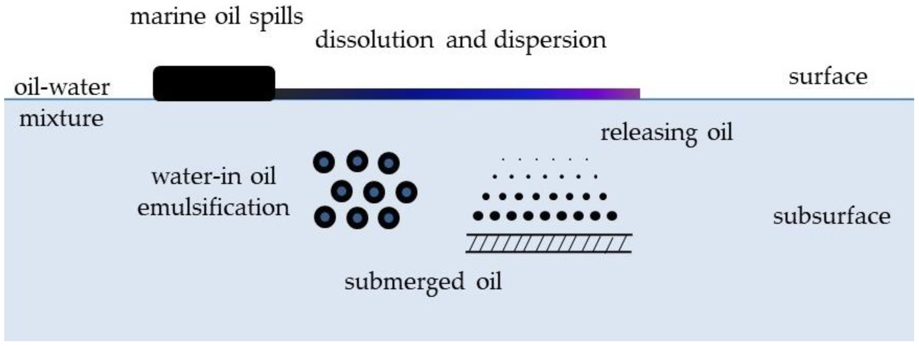
2. Related Works
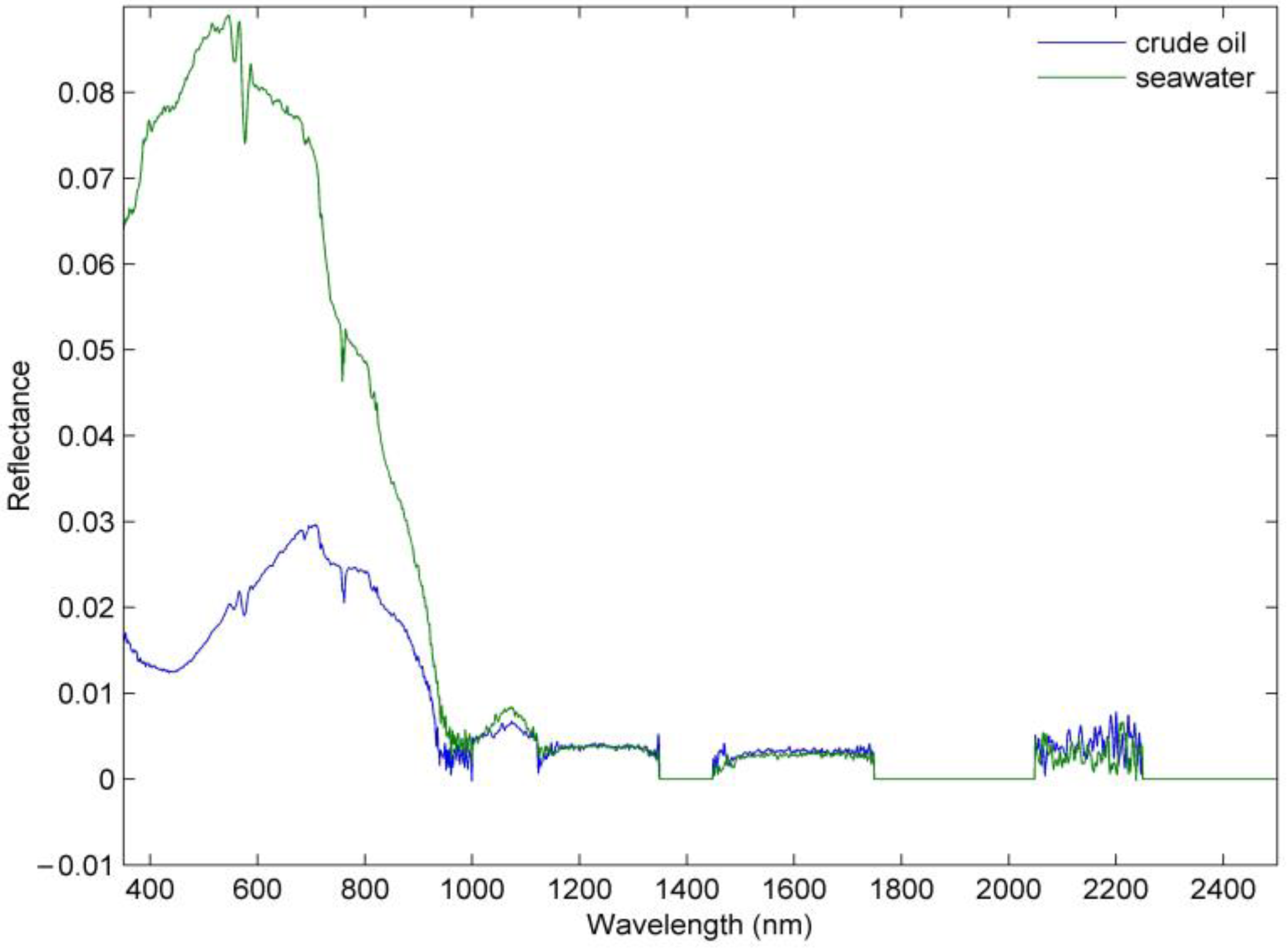
3. Methods
3.1. Normalized PSM
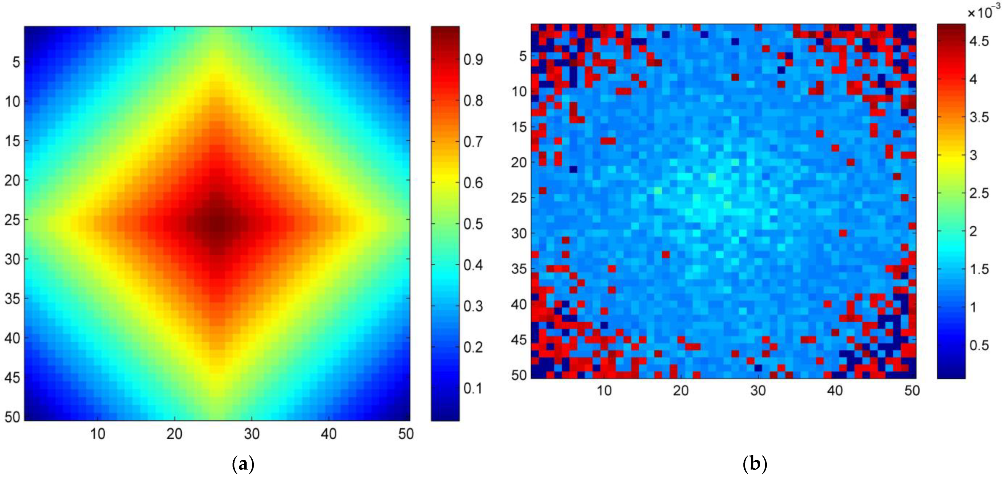
3.2. Energy-Based Wavelet Package Decomposition Method
3.3. ENPSM Unmixing Method
4. Experiments and Results
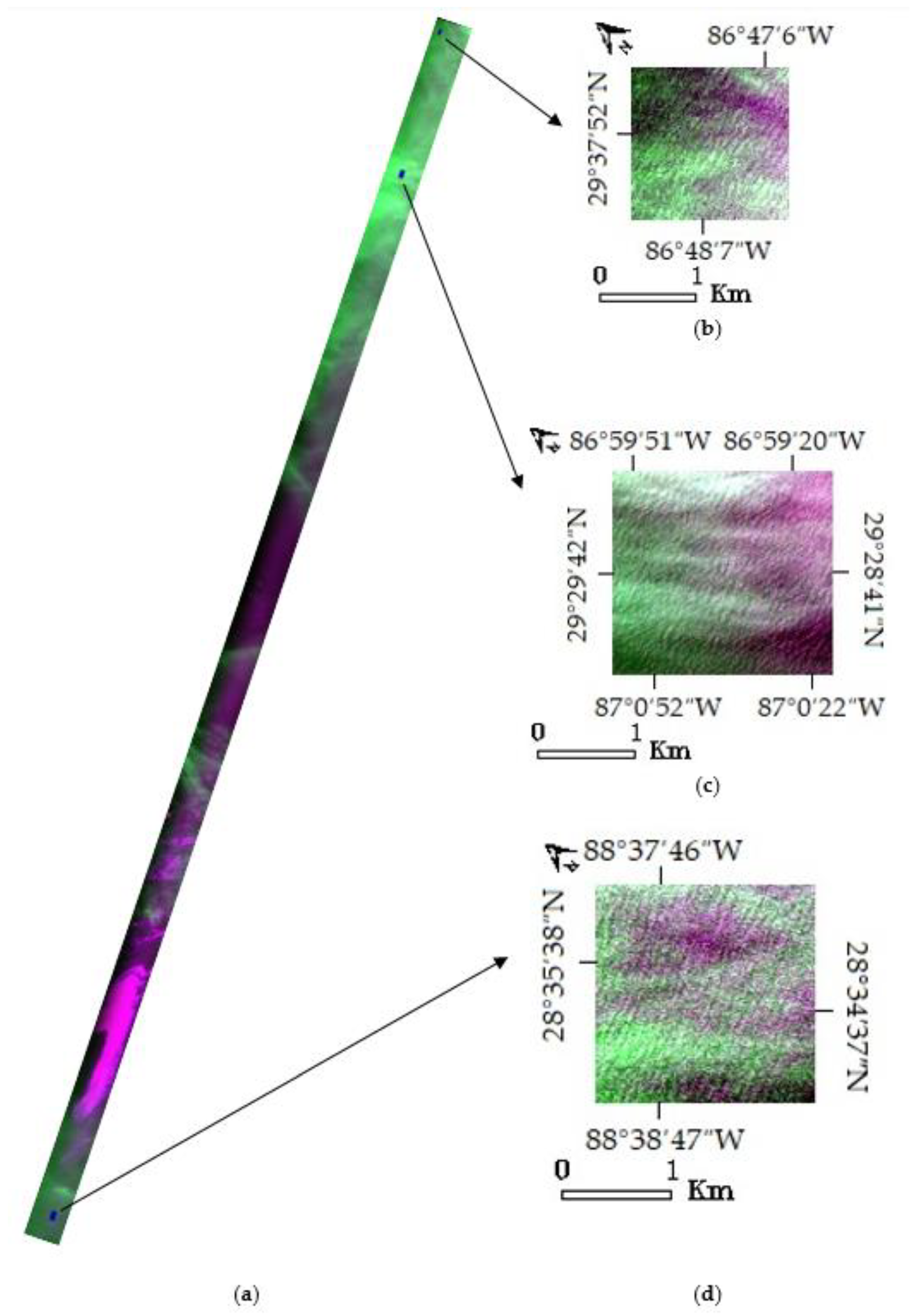
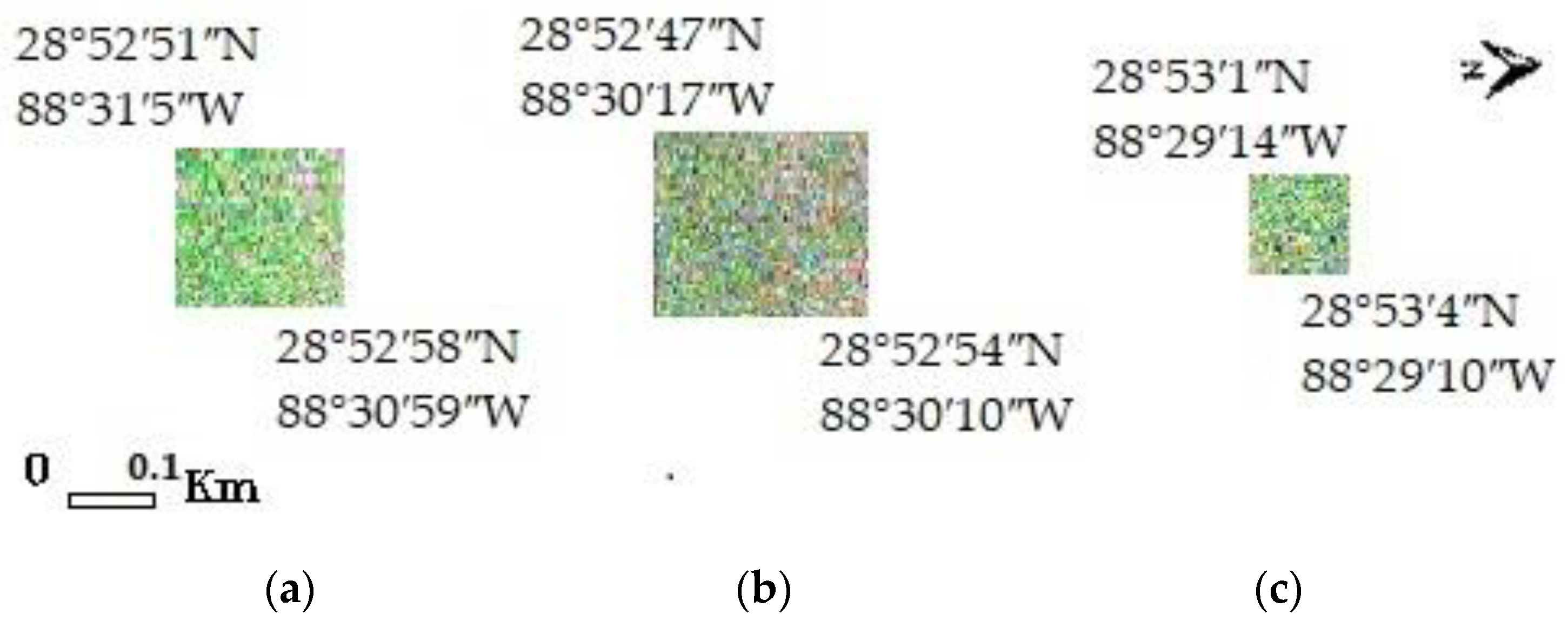
4.1. Experimental Data
4.2. Validation Approach
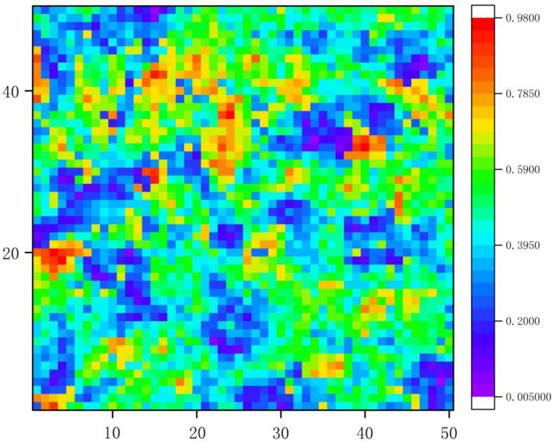
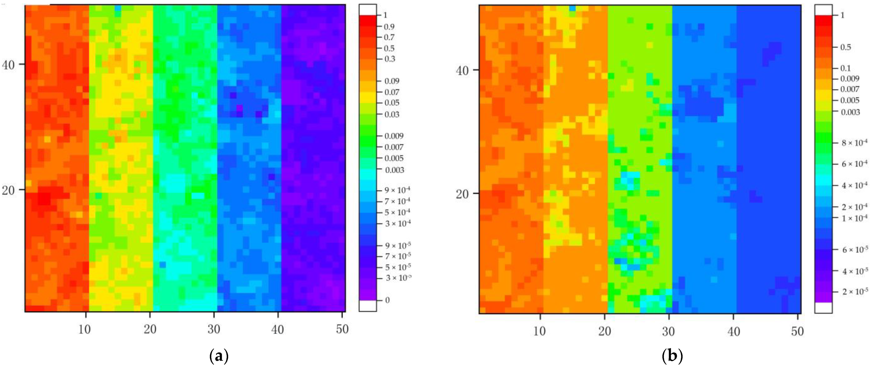
4.3. Synthetic Data
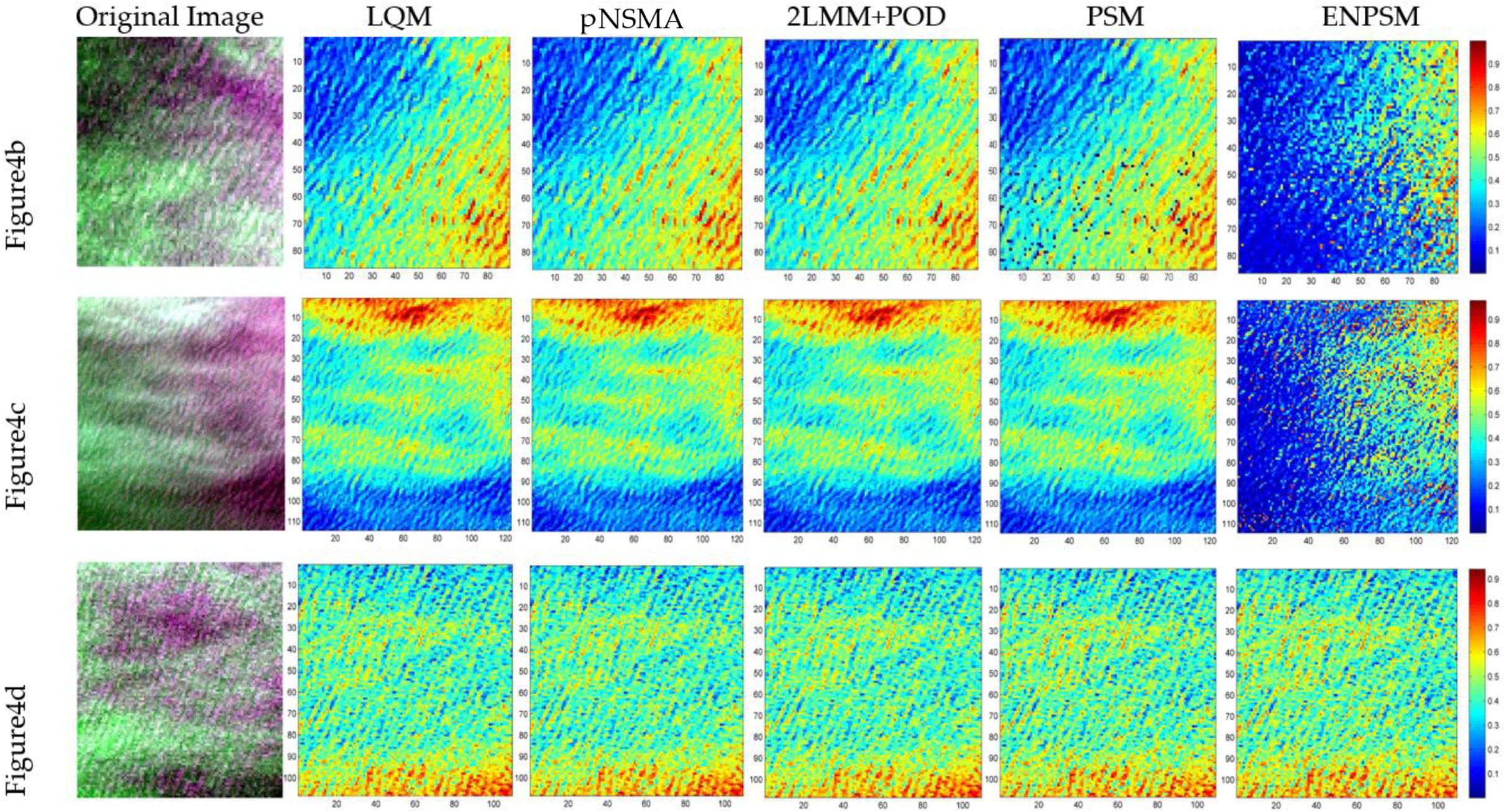
4.4. Oil Spill in the Gulf of Mexico
4.5. Constructed Oil Spill Imagery
5. Discussion
5.1. Comparison of Three Validation Approaches
5.2. Comparison of Five Unmixing Methods
5.3. Limitation
6. Conclusions
Author Contributions
Funding
Conflicts of Interest
References
- Irving, A.; Mendelssohn, G.L.A.; Donald, M.B.; Rex, H.C.; Kevin, R.C.; John, W.F.; Samantha, B.J.; Qianxin, L.; Edward, M.; Edward, B.O.; et al. Oil Impacts on Coastal Wetlands: Implications for the Mississippi River Delta Ecosystem after the Deepwater Horizon Oil Spill. BioScience 2012, 62, 562–574. [Google Scholar] [CrossRef]
- Whitehead, A.; Dubansky, B.; Bodinier, C.; Garcia, T.I.; Miles, S.; Pilley, C.; Raghunathan, V.; Roach, J.L.; Walker, N.; Walter, R.B.; et al. Genomic and physiological footprint of the Deepwater Horizon oil spill on resident marsh fishes. Proc. Natl. Acad. Sci. USA 2012, 109, 20298–20302. [Google Scholar] [CrossRef] [Green Version]
- Dimitri, V.; Anusha, R.; Swapan, P.; Gonasageran, N. Oil induces chlorophyll deficient propagules in mangroves. Mar. Pollut. Bull. 2020, 150, 1–5. [Google Scholar] [CrossRef]
- Chelsea, C.; Lauren, L.; Charles, B.; Michael, K.; Fernando, G. Transgenerational effects of parental crude oil exposure on the morphology of adult Fundulus grandis. Aquat. Toxicol. 2022, 249, 106209. [Google Scholar] [CrossRef]
- Culbertson, J.B.; Valiela, I.; Pickart, M.; Peacock, E.E.; Reddy, C.M. Long-term consequences of residual petroleum on salt marsh grass. J. Appl. Ecol. 2008, 45, 1284–1292. [Google Scholar] [CrossRef]
- Gilfillan, E.S.; Maher, N.P.; Krejsa, C.M.; Lanphear, M.E.; Ball, C.D.; Meltzer, J.B.; Page, D.S. Use of remote sensing to document changes in marsh vegetation following the Amoco Cadiz oil spill (Brittany, France, 1978). Mar. Pollut. Bull. 1995, 30, 780–787. [Google Scholar] [CrossRef]
- Kokaly, R.F.; Couvillion, B.R.; Holloway, J.M.; Roberts, D.A.; Ustin, S.L.; Peterson, S.H.; Khanna, S.; Piazza, S.C. Spectroscopic remote sensing of the distribution and persistence of oil from the Deepwater Horizon spill in Barataria Bay marshes. Remote Sens. Environ. 2013, 129, 210–230. [Google Scholar] [CrossRef] [Green Version]
- Peterson, S.H.; Roberts, D.A.; Beland, M. Oil detection in the coastal marshes of Louisiana using MESMA applied to band subsets of AVIRIS data. Remote Sens. Environ. 2015, 159, 222–231. [Google Scholar] [CrossRef]
- Ira, L.; Lehr, W.J.; Debra, S.-B. State of the art satellite and airborne marine oil spill remote sensing: Application to the BP Deepwater Horizon oil spill. Remote Sens. Environ. 2012, 124, 185–209. [Google Scholar] [CrossRef] [Green Version]
- Bingxin, L.; Ying, L.; Chengyu, L.; Feng, X.; Jan-Peter, P. Hyperspectral features of oil polluted sea ice and the response to the contamination area fraction. Sensors 2018, 18, 234. [Google Scholar] [CrossRef] [Green Version]
- Xudong, K.; Zihao, W.; Puhong, D.; Xiaohui, W. The Potential of Hyperspectral Image Classification for Oil Spill Mapping. IEEE Trans. Geosci. Remote Sens. 2022, 60, 5538415. [Google Scholar] [CrossRef]
- Dobigeon, N.; Tourneret, J.Y.; Richard, C.; Bermudez, J.C.M.; McLaughlin, S.; Hero, A.O. Nonlinear Unmixing of Hyperspectral Images. IEEE Signal Process. Mag. 2014, 31, 82–94. [Google Scholar] [CrossRef] [Green Version]
- Seyyedsalehi, S.F.; Rabiee, H.R.; Soltani-Farani, A.; Zarezade, A. A Probabilistic Joint Sparse Regression Model for Semisupervised Hyperspectral Unmixing. IEEE Geosci. Remote Sens. Lett. 2007, 14, 592–596. [Google Scholar] [CrossRef]
- Johannes, R.; Knut-Frode, D.; Helene, A.; Tor, N.J.S.; Cathleen, E.J.; Camilla, B. The effect of vertical mixing on the horizontal drift of oil spills. Ocean. Sci. 2018, 14, 1581–1601. [Google Scholar] [CrossRef] [Green Version]
- Gruninger, J.; Ratkowski, A.J.; Hoke, M.L. The sequential maximum angle convex cone (SMACC) endmember model. In Proceedings of the Conference on Algorithms and Technologies for Multispectral, Hyperspectral, and Ultraspectral Imagery X, Orlando, FL, USA, 12–15 April 2004. [Google Scholar]
- Nascimento, J.M.; Dias, J.M.B. Vertex component analysis: A fast algorithm to unmix hyperspectral data. IEEE Trans. Geosci. Remote Sens. 2005, 43, 898–910. [Google Scholar] [CrossRef] [Green Version]
- Jun, L.; Dias, J.M.B. Minimum volume simplex analysis: A fast algorithm to unmix hyperspectral data. In Proceedings of the 2008 IEEE International Geoscience and Remote sensing Symposium (IGARSS), Boston, MA, USA, 6–11 July 2008. [Google Scholar]
- Hapke, B. Bidirectional reflectance spectroscopy. I. Theory. J. Geophys. Res. 1981, 86, 3039–3054. [Google Scholar] [CrossRef] [Green Version]
- Hapke, B. Bidirectional reflectance spectroscopy, 3: Correction for macroscopic roughness. Icarus 1984, 59, 41–59. [Google Scholar] [CrossRef] [Green Version]
- Hapke, B. Bidirectional reflectance spectroscopy, 4: The extinction coefficient and opposition effect. Icarus 1986, 67, 264–280. [Google Scholar] [CrossRef] [Green Version]
- Hapke, B. Scattering and diffraction of light by particles in planetary regoliths. J. Quant. Spectrosc. Radiat. Transf. 1999, 61, 565–581. [Google Scholar] [CrossRef]
- Draine, B.T. The discrete-dipole approximation and its application to interstellar graphite grains. Astrophys. J. 1988, 333, 848–872. [Google Scholar] [CrossRef]
- Shkuratov, Y.; Starukhina, L.; Hoffmann, H.; Arnold, G. A model of spectral albedo of particulate surfaces: Implication to optical properties of the moon. Icarus 1999, 137, 235–246. [Google Scholar] [CrossRef]
- Meganem, I.; Deliot, P.; Briottet, X.; Deville, Y.; Hosseini, S. Linear-quadratic mixing model for reflectances in urban environments. IEEE Trans. Geosci. Remote Sens. 2014, 52, 544–558. [Google Scholar] [CrossRef]
- Somers, B.; Cools, K.; Delalieux, S.; Stuckens, J.; Van der Zande, D.; Verstraeten, W.W.; Coppin, P. Nonlinear Hyperspectral Mixture Analysis for tree cover estimates in orchards. Remote Sens. Environ. 2009, 113, 1183–1193. [Google Scholar] [CrossRef]
- Nascimento, J.M.P.; Dias, J.M.B. Nonlinear mixture model for hyperspectral unmixing. In Proceedings of the SPIE Image Signal Processing for Remote Sensing XV, Berlin, Germany, 28 September 2009. [Google Scholar]
- Kothandaraman, N.; Kaliaperumal, V. Combined particle swarm optimization and modified bilinear model (PSO-MBM) algorithm for nonlinearity detection and spectral unmixing of satellite imageries. Int. J. Remote Sens. 2021, 42, 5194–5213. [Google Scholar] [CrossRef]
- Xiangming, J.; Maoguo, J.; Tao, J.; Mingyang, J. Multiobjective Endmember Extraction Based on Bilinear Mixture Model. IEEE Trans. Geosci. Remote Sens. 2020, 58, 8192–8210. [Google Scholar] [CrossRef]
- Altmann, Y.; Halimi, A.; Dobigeon, N.; Tourneret, J.-Y. Supervised Nonlinear Spectral Unmixing Using a Postnonlinear Mixing Model for Hyperspectral Imagery. IEEE Trans. Image Pross. 2012, 21, 3017–3025. [Google Scholar] [CrossRef] [PubMed] [Green Version]
- Marinoni, A.; Gamba, P. On the Direct Assessment of endmember fractions in hyperspectral images. In Proceedings of the IGARSS 2017, Fort Worth, TX, USA, 23–28 July 2017. [Google Scholar]
- Marinoni, A.; Plaza, J.; Plaza, A.; Gamba, P. Nonlinear Hyperspectral Unmixing Using Nonlinearity Order Estimation and Polytope Decomposition. IEEE J. Sel. Top. Appl. Earth Obs. Remote Sens. 2015, 8, 2644–2654. [Google Scholar] [CrossRef]
- Marinoni, A.; Gamba, P. A novel approach for efficient p-linear hyperspectral unmixing. IEEE J. Sel. Top. Signal Process. 2015, 9, 1156–1168. [Google Scholar] [CrossRef]
- Marinoni, A.; Gamba, P. Accurate Detection of Anthropogenic Settlements in Hyperspectral Images by Higher Order Nonlinear Unmixing. IEEE J. Sel. Top. Appl. Earth Obs. Remote Sens. 2016, 9, 1792–1801. [Google Scholar] [CrossRef]
- Ying, L.; Huimin, L.; Zhenduo, Z.; Peng, L. A novel nonlinear hyperspectral unmixing approach for images of oil spills at sea. Int. J. Remote Sens. 2020, 41, 4684–4701. [Google Scholar] [CrossRef]
- Taichi, T.; Isao, N.; Yoshiko, M.; Yasuhiro, W. Sliding-Window Normalization to Improve the Performance of Machine-Learning Models for Real-Time Motion Prediction Using Electromyography. Sensor 2022, 22, 5005. [Google Scholar] [CrossRef]
- Yuquan, G.; Lei, L.; Ji, Z.; Ying, L. Spatial-spectral sparse unmixing for hyperspectral imagery based on graph Laplacian. Proc. SPIE 2021, 12064, 1206408. [Google Scholar] [CrossRef]
- Zhou, K.; Lei, D.; He, J.; Zhang, P.; Bai, P.; Zhu, F. Single micro-damage identification and evaluation in concrete using digital image correlation technology and wavelet analysis. Constr. Build. Mater. 2021, 267, 120951. [Google Scholar] [CrossRef]
- He, S.-F.; Zhou, Q.; Wang, F. Local wavelet packet decomposition of soil hyperspectral for SOM estimation. Infrared Phys. Technol. 2022, 125, 104285. [Google Scholar] [CrossRef]
- Uttam, K.; Sangram, G.; Ramakrishna, R.N.; Kumar, S.R.; Cristina, M.; Ruchita, S.; Andrew, M.; Petr, V.; Hirofumi, H.; Shuang, L.; et al. Exploring subpixel learning algorithms for estimating global land cover fractions from satellite data using high performance computing. Remote Sens. 2017, 9, 1105. [Google Scholar] [CrossRef] [Green Version]
- Li, Y.; Huang, W.; Lyu, X.; Liu, S.; Zhao, Z.; Ren, P. An adversarial learning approach to forecasted wind field correction with an application to oil spill drift prediction. Int. J. Appl. Earth Obs. Geoinf. 2022, 112, 102924. [Google Scholar] [CrossRef]
- Marinoni, A.; Plaza, A.; Gamba, P. Harmonic mixture modeling for efficient nonlinear hyperspectral unmixing. IEEE J. Sel. Top. Appl. Earth Obs. Remote Sens. 2016, 9, 4247–4256. [Google Scholar] [CrossRef]
- Lu, Y.; Shi, J.; Wen, Y.; Hu, C.; Zhou, Y.; Sun, S.; Zhang, M.; Mao, Z.; Liu, Y. Optical interpretation of oil emulsions in the ocean—Part I: Laboratory measurements and proof-of-concept with AVIRIS observations. Remote Sens. Environ. 2019, 230, 111183. [Google Scholar] [CrossRef]


| Name | Attribute | |
|---|---|---|
| Sensor | AVIRIS | |
| Spectral range (nm) | 380–2500 | |
| Number of bands | 224 | |
| Date of acquisition | 13 May 2010 | |
| Size (pixels) | Figure 4b | 86 × 89 |
| Figure 4c | 114 × 123 | |
| Figure 4d | 108 × 109 | |
| Date of acquisition | 9 July 2010 | |
| Size (pixels) | Figure 5a | 49 × 52 |
| Figure 5b | 57 × 65 | |
| Figure 5c | 31 × 31 | |
| Images | Mixture Model | Magnitude Order | Reconstruction Performance | LQM | pNSMA | 2LMM + POD | PSM | ENPSM |
|---|---|---|---|---|---|---|---|---|
| Image 1 | LQM | RE | 0.0022 | 0.0022 | 0.0022 | 0.0022 | 0.0024 | |
| RMSE | 0.0327 | 0.0439 | 0.0327 | 0.0334 | 0.0929 | |||
| LOGRMSE | 11.9321 | 0.3378 | 0.6974 | 0.5971 | 0.0802 | |||
| Image 2 | LQM | RE | 0.0023 | 0.0022 | 0.0022 | 0.0022 | 0.0028 | |
| RMSE | 0.0318 | 0.0777 | 0.0318 | 0.0334 | 0.0288 | |||
| LOGRMSE | 97.9863 | 298.5316 | 5.7726 | 5.0710 | 0.3350 | |||
| Image 3 | LQM | RE | 0.0022 | 0.0022 | 0.0022 | 0.0022 | 0.0031 | |
| RMSE | 0.0076 | 0.0076 | 0.0076 | 0.0076 | 0.0065 | |||
| LOGRMSE | 290.4378 | 291.6509 | 16.8534 | 40.6913 | 0.7006 | |||
| Image 4 | Hapke | RE | 0.0022 | 0.0022 | 0.0022 | 0.0022 | 0.0027 | |
| RMSE | 0.0451 | 0.0604 | 0.0441 | 0.0445 | 0.0678 | |||
| LOGRMSE | 0.0348 | 0.0662 | 0.0499 | 0.0838 | 0.0568 | |||
| Image 5 | Hapke | RE | 0.0022 | 0.0022 | 0.0022 | 0.0159 | 0.0039 | |
| RMSE | 0.0574 | 0.0591 | 0.0144 | 0.0159 | 0.0190 | |||
| LOGRMSE | 6.8086 | 6.2395 | 4.3820 | 3.9218 | 0.2243 |
| Figure | Unmixing Method | Number of the Underestimated Pixels | LOGRMSE |
|---|---|---|---|
| Figure 1 | LQM | 4 | 0.0414 |
| Figure 2 | 2LMM + POD | 1 | 0.3856 |
| Figure 2 | PSM | 28 | 0.4156 |
| Figure 5 | 2LMM + POD | 162 | 0.2507 |
| Figure 5 | PSM | 182 | 0.2666 |
| Mixture Model | Magnitude Order | LOGRMSE | Mixture Model | Magnitude Order | LOGRMSE |
|---|---|---|---|---|---|
| LQM | 0.0802 | Hapke | 0.0568 | ||
| 0.3350 | 0.2243 | ||||
| 0.7006 | 0.6466 | ||||
| 0.8798 | 0.8671 | ||||
| 0.5249 | 0.9490 |
| Figure | LQM | pNSMA | 2LMM+POD | PSM | ENPSM |
|---|---|---|---|---|---|
| Figure 4b | 0.0138 | 0.0138 | 0.0138 | 0.0206 | 0.0161 |
| Figure 4c | 0.0119 | 0.0119 | 0.0119 | 0.0179 | 0.0481 |
| Figure 4d | 0.0133 | 0.0134 | 0.0133 | 0.0123 | 0.0147 |
Disclaimer/Publisher’s Note: The statements, opinions and data contained in all publications are solely those of the individual author(s) and contributor(s) and not of MDPI and/or the editor(s). MDPI and/or the editor(s) disclaim responsibility for any injury to people or property resulting from any ideas, methods, instructions or products referred to in the content. |
© 2023 by the authors. Licensee MDPI, Basel, Switzerland. This article is an open access article distributed under the terms and conditions of the Creative Commons Attribution (CC BY) license (https://creativecommons.org/licenses/by/4.0/).
Share and Cite
Lu, H.; Li, Y.; Liu, B. Energy-Based Unmixing Method for Low Background Concentration Oil Spills at Sea. Remote Sens. 2023, 15, 2079. https://doi.org/10.3390/rs15082079
Lu H, Li Y, Liu B. Energy-Based Unmixing Method for Low Background Concentration Oil Spills at Sea. Remote Sensing. 2023; 15(8):2079. https://doi.org/10.3390/rs15082079
Chicago/Turabian StyleLu, Huimin, Ying Li, and Bingxin Liu. 2023. "Energy-Based Unmixing Method for Low Background Concentration Oil Spills at Sea" Remote Sensing 15, no. 8: 2079. https://doi.org/10.3390/rs15082079