Article

Unsupervised Affinity Propagation Clustering Based Clutter Suppression and Target Detection Algorithm for Non-Side-Looking Airborne Radar

1
National Key Laboratory of Radar Signal Processing, Xidian University, Xi’an 710071, China
2
Computer Science Program, University of Southampton Malaysia, Nusajaya 79100, Malaysia
*
Author to whom correspondence should be addressed.
Remote Sens. 2023, 15(8), 2077; https://doi.org/10.3390/rs15082077
Submission received: 3 March 2023 / Revised: 6 April 2023 / Accepted: 11 April 2023 / Published: 14 April 2023

Abstract

:
Aimingat non-side-looking airborne radar, we propose a novel unsupervised affinity propagation (AP) clustering radar detection algorithm to suppress clutter and detect targets. The proposed method first uses selected power points as well as space-time adaptive processing (STAP) weight vector, and designs matrix-transformation-based weighted input data, with which the first unsupervised weighted AP clustering is proposed by means of their similarity matrix, responsibility values and availability values. Then, new reconstructed weighted power inputs are designed, and the second weighted AP clustering is proposed. Finally, with their cluster results, a detection-discriminant criterion is designed for the judgment of target detection, and simultaneously, the clutter is suppressed. Compared with the conventional and important STAP, ADC and JDL algorithms, and several SO-based, GO-based and OS-based CFAR algorithms, the proposed unsupervised algorithm achieves much higher probability of detection and provides distinctly superior target-detection performance. With reasonable computation time, it can better conquer the range dependence in characteristic of clutter and better process non-independent identically distributed (non-IID) samples of non-side-looking radar. Sufficient simulations are performed, and they demonstrate that the proposed unsupervised algorithm is preferable and advantageous.

1. Introduction

Airborne radar garners considerable attention on account of its flexibility and long field of view, but it suffers from the core problem that the strong clutter and its broadened spectrum drowns out weak targets [1,2,3,4]. To deal with clutter and detect targets, the leading technology known as space-time adaptive processing (STAP) [4,5,6] achieves this by estimating the accurate covariance matrix of clutter and noise in applications, and sufficient samples are also required to be independent identically distributed (IID). However, by reason of radar configuration and signal environment, practical clutter characteristics are usually non-uniform, which results in significant degradation of performance for traditional methods of suppressing the clutter and detecting the target. Particularly when the antenna array of airborne radar is configured as non-side-looking, the samples directly cause a failure in IID due to range dependence of clutter [7].
In the range-compensation methods, the common aim is to make the compensated clutter spectra be consistent with each other [8,9,10]. For example, a Doppler warping (DW) method [11,12] is proposed for a non-side-looking array by exploiting the radar navigation parameters. It shifts the two-dimensional clutter spectrum into a one-dimensional spectrum, with which the spectrum becomes coincident with that to be detected upon the direction of Doppler. In addition, a well-known ADC algorithm that is angle Doppler compensation [13] uses an inertial navigation parameter and linear transformation; then, the broadened clutter is improved. In addition to those methods, a high-order Doppler warping (HODW) method [14] considers multiple spatial angle directions to compensate the adjacent range cells. However, most of the existing range-compensation methods rely heavily on the given and the estimated multiple parameters of the inertial navigation system, which indicates that they tend to be non-adaptive methods.
For purpose of overcoming the non-IID condition of clutter characteristic in non-side-looking radar, dimension- and rank-reduction methods usually reduce degrees of freedom (DOF) and select partial samples [15,16,17]. The classical joint domain localized (JDL) algorithm [18] brings in Fourier transformation with two dimensions and picks out a rectangular local region for joint processing. It is worth stressing that the JDL method processes the beamforming and the Doppler frequency simultaneously. Moreover, by constructing the auxiliary beam, the auxiliary cannel processing (ACP) method [19] lessens the system’s DOF from N K to N + K 1 , where N is the number of array elements and K is the number of transmitted pulses in a coherent processing interval. However, reduction of the sample data and the system’s DOF directly leads to performance degradations when suppressing the clutter and detecting the target in the above methods.
Aiming at target detection for airborne radar, a number of methods have been proposed, including the commonly applied constant false alarm rate (CFAR) extended methods [20,21,22,23,24,25,26,27,28], such as cell averaging CFAR (CA-CFAR) [22]; the smallest of CFAR method—that is, SO-CFAR [23]; the greatest of CFAR, abbreviated as GO-CFAR [24]; and order statistic CFAR, abbreviated as OS-CFAR [25]. It is worth mentioning that machine learning developments have contributed some algorithms in signal processing of radar. However, most of the machine learning-based target-detection methods [29,30] for airborne radar concentrate on processing and optimization for synthetic aperture radar (SAR) image. Meanwhile, they usually require a number of labeled data and cannot be directly applied to clutter suppression and target detection for non-side-looking radar with non-IID samples—on which there is also little related clustering literature—although the unsupervised clustering algorithms [31] of machine learning do not require labeled data. For example, an affinity propagation method [32] achieves unsupervised clustering while having no need for specifying the number of clusters in advance, and it finds the final cluster centers from existing data points rather than creating new data points. Moreover, it is insensitive to the initial values of the data. However, when specially applied to radar receive data, the clustering methods suffer challenges, including the design of appropriate input data points, relevant clustering parameters and particular criteria for clutter suppression and target detection. A few of other machine learning-based methods [33,34,35,36] for clutter suppression have been proposed, but they mainly aim at suppressing the clutter by improving the estimation of the clutter characteristics, rather than directly detecting the target by proposing target and clutter classifiers.
To solve these problems mentioned above, an unsupervised affinity propagation (AP) clustering based clutter-suppression and target-detection algorithm for non-side-looking airborne radar is proposed. The work presented here exploits the advantages of machine learning technologies to directly propose a machine learning-based target-detection algorithm, which is suited to airborne non-side-looking radar whose samples are non-IID, and it can detect the target and suppress the clutter simultaneously. Meanwhile, it is an unsupervised algorithm that does not require any labeled data or assigned labels.
Directed at non-side-looking radar, this novel method first uses matrix transformation based on the STAP weight vector and the selected power points including clutter plus noise and signal, and designs weighted input data for target detection. Next, the first unsupervised weighted AP clustering is proposed for the whole designed weighted input, by means of their similarity matrix, responsibility values and availability values. Then, the proposed method designs new reconstructed weighted power input, with which the second weighted AP clustering is further proposed. Finally, with the cluster results of the first and the second weighted AP clusterings, a target detection-discriminant criterion is designed. The proposed unsupervised algorithm can effectively and advantageously detect the target, and simultaneously suppress clutter. Compared with conventional clutter-suppression and target-detection methods, including the STAP, ADC, JDL and several CFAR-based methods, the proposed unsupervised algorithm implements greatly superior target detection and a distinctly higher probability of detection (PD). With reasonable computation time, it better conquers the range dependence of the characteristics of the clutter and better deals with the non-IID-sample circumstance of non-side-looking radar.

2. Signal Model

Consider that the array of airborne radar system is uniform and linear, and it is equipped with N receiving array elements, whose element inner space is generally a half-wavelength represented as d = λ / 2 . In a certain coherent processing interval, the number of transmitted pulses is K, which is specific to a certain pulse repetition frequency. The uniform speed of the moving airborne platform is denoted as v a . Moreover, ϑ is used to represent the non-side-looking angle. Therefore, we have [37,38,39]
a t ( f ¯ d , i ) = [ 1 , e j 2 π f ¯ d , i , , e j 2 π ( K 1 ) f ¯ d , i ]
and
a s ( f ¯ s , i ) = [ 1 , e j 2 π f ¯ s , i , , e j 2 π ( N 1 ) f ¯ s , i ]
where a t ( f ¯ d , i ) and a s ( f ¯ s , i ) stand for temporal and spatial steering vectors, respectively; meanwhile, f ¯ d , i and f ¯ s , i are the normalized Doppler and spatial frequencies, respectively. Then, corresponding to the ith block of clutter, we have
a s t ( f ¯ s , i , f ¯ d , i ) = a t ( f ¯ d , i ) a s ( f ¯ s , i ) C N K × 1
where a s t ( f ¯ s , i , f ¯ d , i ) C N K × 1 denotes the space-time steering vector with dimensions N K × 1 , and ⊗ is the Kronecker product. Based on this, we can express the stacked echo data vector as follows [37]:
x c n , l = i = 1 N c ξ i , l a s t ( f ¯ s , i , f ¯ d , i ) + n l
where scalar l stands for the lth range cell attached to the total L training range cell samples, and vector n l denotes noise with a zero mean. Additionally, N c is the total number of clutter blocks subject to a certain clutter cell; meanwhile, { ξ 1 , l , ξ 2 , l , , ξ N c , l } are their respective complex amplitudes. Then, making use of L training samples and by maximum likelihood estimation, covariance matrix with regard to x c n , l is [40]
R X R ^ X 1 L 1 l = 1 , l l s L x c n , l x c n , l H
where R ^ X is the covariance estimation matrix and ( · ) H is the conjugate transpose. It excludes x c n , l s , which is the sample that may contain the target. Then, to suppress clutter for further target detection, utilizing Lagrange multiplier technology, by solving the minimized variance problem { min w w H R X w , s . t . w H a s t ( f s 0 , f d 0 ) = 1 } , STAP calculates its weight vector w o p t , as follows [37]:
w o p t = R X 1 a s t ( f s 0 , f d 0 ) a s t H ( f s 0 , f d 0 ) R X 1 a s t ( f s 0 , f d 0 )
where ( · ) 1 is an inverse operation. N K × 1 -dimensional a s t ( f s 0 , f d 0 ) corresponds to the target, whose temporal frequency and spatial frequency are f d 0 and f s 0 , respectively. Hence, by adding the weight vector w o p t to the received data x c n , l , further target detection performance of STAP can be achieved by detection methods. Generally, target detection of radar is a binary hypothesis problem, which corresponds to hypotheses H 0 and H 1 on behalf of nonexistence and existence of the target, respectively—that is [25,26,27],
H 0 : x l = x c n , l , | x l | η 0 H 1 : x l = x c n , l + x s , l , | x l | > η 0
where x c n , l is composed of clutter plus noise, x s , l is the received target echo, and for STAP, x l is replaced by w o p t H x l . Moreover, η 0 = T h × Z c n is the threshold value of detection, with T h and Z c n being the threshold factor and the clutter-plus-noise power level. Specifically, as one of the classical methods of target detection, the OS-CFAR detection method estimates Z c n by firstly processing the order of the selected R reference cell samples from small to large x 1 x 2 x R , and then the R K th ordered sample x R K becomes the judgment threshold for total clutter-plus-noise power. This can be written as [23]
Z c n = α x R K
where α is the scale factor, whose value is related to the false-alarm probability. Unfortunately, target detection is degraded seriously when the estimated power Z c n is inaccurate. The most significant reason is the non-IID training sample circumstance in non-side-looking radar. In this case, clutter distribution changes along with the range, and the clutter statistics for different range cells are not identical. Traditional dimension and rank reduction methods solve this problem at the expense of a reduction in the system’s degree of freedom, and the clutter suppression STAP method suffers degradation on account of inaccurate estimation of R X . In addition, traditional range-compensation methods for this problem usually rely heavily on the multiple parameters of the inertial navigation system, and they are non-adaptive methods.

3. The Proposed Algorithm

The proposed method designs an unsupervised, weighted AP clustering algorithm for detecting targets in clutter, relying on clustering different clutter and target data twice, which are exploited to further the detection discriminant criterion based on AP clustering. Specifically, the power points including clutter, noise and signal, are brought in first, as follows:
P o w S ( l , m ) = 1 a s t H ( f ¯ s l , f ¯ d m ) R X S a s t ( f ¯ s l , f ¯ d m )
where P o w S ( l , m ) stands for the ( l , m ) th element of the matrix P o w S C L × M composed of the power points, and different from R X for clutter plus noise, R X S is derived from all samples that may contain detected targets. Furthermore, f ¯ d m in a s t ( f ¯ s l , f ¯ d m ) , derived from Equation (3), denotes the normalized Doppler frequency corresponding to the mth point in the interested temporal domain, whose total number of the assigned points is M. Meanwhile, f ¯ s l represents the lth normalized spatial frequency of the power points in the spatial distribution. In the matrix P o w S C L × M , L can be set as the number introduced after Equation (4) for more easily comprehending the further design of weighted operation. Then, the weights used to construct the weighted data as the input of the designed clustering for clutter plus noise and target are proposed as
E c n s ( l ) = ( ϖ m a x ϖ m i n ) ( w o p t H x c n , l min { w o p t H X c n s } ) max { w o p t H X c n s } min { w o p t H X c n s } + ϖ m i n
for l = 1 , 2 , , L , and w o p t can be obtained from Equation (6). Moreover, max { · } stands for taking the maximum, whereas min { · } stands for taking the minimum. For Equation (10), ϖ m a x and ϖ m i n are the desired maximum and minimum after the normalization. With E c n s , the weight matrix E ^ c n s in the proposed method is organized as
E ^ c n s = [ E c n s ( 1 ) , E c n s ( 2 ) , , E c n s ( L ) ; ; E c n s ( 1 ) , E c n s ( 2 ) , , E c n s ( L ) ] C M × L
where L has been defined after Equation (4). Hence, the final weighted data for the proposed detection clustering are designed as follows:
F ^ w ( m , l ) = [ 10 log 10 ( | P o w S | D m a x ) ] H ( m , l ) [ E ^ c n s ( m , l ) ] η
with which the final weighted input matrix is
F ^ ˜ w = | F ^ w | max { | F ^ w | }
where in Equations (12) and (13), | · | denotes the absolute value matrix for each of its elements, and D m a x = max { | P o w S | } . In addition, [ · ] ( m , l ) and [ · ] η are the ( m , l ) th element and the η th power of [ · ] , respectively, and 10 log 10 ( · ) is the logarithmic function. The setting of η , ϖ m a x , and ϖ m i n adjust the effect of the weights E ^ c n s ( m , l ) on the constructed weighted input data for the detection clustering.
The proposed weighted AP clustering algorithm for radar clutter suppression and target detection performs the clustering twice and then designs the detection-discriminant criterion, by which the consequence of clutter is eliminated and the target can be detected. The first AP clustering is based on the whole designed weighted input data F ^ ˜ w , and affinity propagation is clustered on the similarity matrix of these data points. The AP clustering treats all of the inputs as possible cluster centers, which are called exemplars. Since the goal of clustering is to minimize distance, the Euclidean distance can be chosen as the metrics of similarity—that is, the similarity of any two points is written as
s ( i , j ) = d E 2 [ F ^ ˜ w ( i , : ) , F ^ ˜ w ( j , : ) ] = l = 1 L [ F ^ ˜ w ( i , l ) F ^ ˜ w ( j , l ) ] 2 , i j
where F ^ ˜ w ( i , : ) represents a certain row and { i , j } = 1 , 2 , , M . The similarity s ( i , j ) can form a similarity matrix S C M × M . When i = j , s ( i , j ) is defined as
s ( i , j ) = P i , i = j
where P i is known as the preference, whose value and the maximum iteration number T can be assigned. The proposed unsupervised algorithm sets the ith preference element P i as
P i = p r e · mean { S ˜ } , i = 1 , 2 , , M
where p r e is the adjustment parameter for the preference and mean { · } stands for the mean of all the elements in { · } . Furthermore, the detailed representation of S ˜ is
S ˜ = s ( 1 , 2 ) s ( 1 , 3 ) s ( 1 , 4 ) s ( 1 , M ) s ( 2 , 1 ) s ( 2 , 3 ) s ( 2 , 4 ) s ( 2 , M ) s ( 3 , 1 ) s ( 3 , 2 ) s ( 3 , 4 ) s ( 3 , M ) s ( M , 1 ) s ( M , 2 ) s ( M , 3 ) s ( M , M 1 ) C M × ( M 1 )
Next, based on s ( i , j ) , to achieve the clustering of the clutter plus noise and signal, it is important to calculate the responsibility value ( i , j ) and the availability value β ( i , j ) for the data points F ^ ˜ w . They represent different categories of data information. More specifically, with respect to point i, ( i , j ) stands for the degree of suitability of point j serving as its exemplar, and ( i , j ) is expressed in detail as [32]
( i , j ) = s ( i , j ) max h j { s ( i , h ) + β ( i , h ) } , h = 1 , 2 , , M
where the initial value of β ( i , h ) is zero. Particularly, we directly have
( j , j ) = p r e · mean { S ˜ } max h j { s ( j , h ) + β ( j , h ) }
for i = j . On the other hand, for the availability β ( i , j ) , as the other evaluation information between different points, it stands for the degree of suitability that point i picks j as the exemplar, and it is calculated from
β ( i , j ) = min { 0 , ( j , j ) + p i , p j max { 0 , ( p , j ) } } , i j , p = 1 , 2 , , M
and otherwise
β ( i , j ) = β ( j , j ) = p j max { 0 , ( p , j ) } , i = j
where 1 p M . The iterative processing of AP clustering is alternately updating ( i , j ) and β ( i , j ) . To avoid oscillations, a damping factor λ [ 0.5 , 1 ) is introduced, and the stability of the iterative process can be guaranteed. With the damping factor, the updating of ( i , j ) for i j is expressed as
( t ) ( i , j ) = λ ( t 1 ) ( i , j ) + ( 1 λ ) [ s ( i , j ) max h j { s ( i , h ) + β ( t ) ( i , h ) } ]
where t T , and the updating of β ( i , j ) for i j is
β ( t ) ( i , j ) = λ β ( t 1 ) ( i , j ) + ( 1 λ ) [ min { 0 , ( t ) ( j , j ) + p i , j max { 0 , ( t ) ( p , j ) } } ]
where above ( t ) ( i , j ) and β ( t ) ( i , j ) are the updated ( i , j ) and β ( i , j ) for the tth iteration containing the damping factor. Meanwhile, the special circumstance for i = j should be separately calculated as the following different results:
( t ) ( j , j ) = λ ( t 1 ) ( j , j ) + ( 1 λ ) [ p r e · mean { S ˜ } max h j { s ( j , h ) + β ( t ) ( j , h ) } ]
where the adjustment parameter p r e will be designed especially by the proposed unsupervised algorithm. In addition, another result for i = j is
β ( t ) ( j , j ) = λ β ( t 1 ) ( j , j ) + ( 1 λ ) [ p j max { 0 , ( t ) ( p , j ) } ]
Hence, AP clustering determines the exemplar by combining the reliability ( i , j ) and the validity β ( i , j ) . That is, when a certain point j makes ( i , j ) + β ( i , j ) reach the maximum value, we have
I j = arg j max { ( t ) ( i , j ) + β ( t ) ( i , j ) } , i
together with
Q 1 = num { I 1 , I 2 , , I Q 1 }
where I j is regarded as cluster center of the ith point; in addition, arg max { · } finds the argument for maximization and num { · } counts the total number of elements. With the defining of Q 1 , the adjustment parameter p r e is specially pointed out, because its design satisfies
| arg p r e { Q 1 = 2 } | < p r e | arg p r e { Q 1 = 1 } |
where p r e is a positive value. Larger preference P i contributes to more final cluster centers [32]; meanwhile, the negative preference P i is obtained from the negative matrix S ˜ and the positive p r e . Therefore, a larger preference P i is obtained from a smaller p r e , which means that the p r e for Q 1 = 2 is smaller than the p r e for Q 1 = 1 .
Finally, if the iteration totality becomes more than the assigned T or cluster centers do not change in several iterations, the first clustering in the proposed unsupervised algorithm can be deemed as finished by taking down the total cluster number Q 1 and their corresponding cluster centers [ I 1 , I 2 , , I Q 1 ] . With regard to the final clusters, their total number Q 1 for the proposed first clustering is controlled as Q 1 = 1 by adjusting the designed preference adjustment parameter p r e in advance.
The proposed method further designs the second clustering by constructing new data input that contains the clutter plus noise. Therefore, the differences between the first clustering and the second clustering are fully utilized to distinguish if there is a target in the non-IID clutter. More specifically, reconstruct the data input for the proposed weighted AP clustering as follows:
Y ˜ w = F ^ ˜ w ( 1 , 1 ) F ^ ˜ w ( 1 , 2 ) F ^ ˜ w ( 1 , M 2 l s e 1 ) F ^ ˜ w ( 2 , 1 ) F ^ ˜ w ( 2 , 2 ) F ^ ˜ w ( 2 , M 2 l s e 1 ) F ^ ˜ w ( M 2 l s e 1 , 1 ) F ^ ˜ w ( M 2 l s e 1 , 2 ) F ^ ˜ w ( M 2 l s e 1 , M 2 l s e 1 ) F ^ ˜ w ( M 2 + l s e 2 , M 2 + l s e 2 ) F ^ ˜ w ( M 2 + l s e 2 , M 2 + l s e 2 + 1 ) F ^ ˜ w ( M 2 + l s e 2 , M ) F ^ ˜ w ( M 2 + l s e 2 + 1 , M 2 + l s e 2 ) F ^ ˜ w ( M 2 + l s e 2 + 1 , M 2 + l s e 2 + 1 ) F ^ ˜ w ( M 2 + l s e 2 + 1 , M ) F ^ ˜ w ( M , M 2 + l s e 2 ) F ^ ˜ w ( M , M 2 + l s e 2 + 1 ) F ^ ˜ w ( M , M )
where l s e 1 and l s e 2 = l s e 1 + 1 are the size parameters, which determine the reconstructed data that remove a number of points, including the removed central entries around F ^ ˜ w ( M / 2 , M / 2 ) . Furthermore, we express the detailed dimension of the designed Y ˜ w as follows:
Y ˜ w C [ M + 1 ( l s e 1 + l s e 2 ) ] × ( M 2 l s e 1 )
Taking advantage of the designed Y ˜ w , the proposed method performs the second clustering expressed as
{ I j Y } j = 1 , 2 , , Q 2 = arg j max { γ i j ( Y ˜ w , P Y ) + α i j ( Y ˜ w , P Y ) }
where γ i j ( Y ˜ w , P Y ) and α i j ( Y ˜ w , P Y ) represent the obtained ( i , j ) and β ( i , j ) with the cluster processing elaborated from Equation (14) to Equation (25) under new input Y ˜ w and new preference P Y . By exploiting the updated preference, Q 2 is the number of the final stable clusters with the corresponding centers [ I 1 Y , I 2 Y , , I Q 2 Y ] . Furthermore, P Y is the preference matrix for the proposed second clustering, and its element P i Y is put forward as
P i Y = p r e Y · P i = p r e Y · p r e · mean { S } , i = 1 , 2 , , M + 1 ( l s e 1 + l s e 2 )
where P i , p r e and S ˜ are defined in Equations (16) and (17), and p r e Y is another adjustment parameter of the preference for the second clustering. Once obtained, Q 1 , Q 2 , [ I 1 , I 2 , , I Q 1 ] and [ I 1 Y , I 2 Y , , I Q 2 Y ] are all used by the proposed method. By exploring and distinguishing their differences, we further design a detection-discriminant criterion for radar detection, as follows:
H 1 : x l = x c n , l + x s , l , when Q 1 = Q 2 = 1 , u d 1 I 1 Y u d 2 , u d 3 I 1 u d 4 H 1 : x l = x c n , l + x s , l , when Q 1 = Q 2 = 1 , I 1 Y = u d 5 , u d 3 I 1 u d 4 H 1 : x l = x c n , l + x s , l , when Q 1 = 1 , Q 2 = 2 , | x l | > η 0 H 0 : x l = x c n , l , otherwise
where hypotheses H 1 and H 0 are, respectively, on behalf of target-existence and target-nonexistence. Moreover, u d 1 to u d 5 are the parameters used to define the judgment interval for target detection, and η 0 is the detection threshold of OS-CFAR. They indicate that when both of the numbers of the cluster centers for the first and the second clusterings are Q 1 = Q 2 = 1 and the two centers are located in their own judgment intervals, and when Q 1 = 1 and Q 2 = 2 with | x l | > η 0 , the proposed method determines the target’s presence. Otherwise, the proposed method determines that there is only clutter and noise in the detected range cell. The conclusion of the processing procedure for the proposed unsupervised detection algorithm can be found in Table 1.

4. Simulation Results

The proposed unsupervised AP algorithm for radar detection in clutter is preferable and advantageous, as verified in the following simulations. Except for the corresponding settings specifically pointed out in some simulations, the system and parameter settings for radar are as follows. For airborne radar, its height is H = 6000 m, its number of array elements is N = 10 and the inner distance is d = 0.3 m. Additionally, the pulse number defined before Equation (1) is K = 10 , and the wavelength is λ = 0.15 m.
In addition, for the proposed method, the parameter settings are p r e = 16.68 , p r e Y = 1.05 , l s e 1 = 5 , l s e 2 = 6 , u d 1 = 8 , u d 2 = 10 , u d 3 = 11 , u d 4 = 30 and u d 5 = 42 , respectively, where p r e and p r e Y are the preferences for the first and second clusterings of the proposed method. In addition, l s e 1 = 5 and l s e 2 = 6 are used for reconstructing the new data of the the second clustering with M = 60 . Meanwhile, u d 1 to u d 5 are the corresponding settings of the judgment interval in the detection-discriminant criterion for target detection. Furthermore, in the following descriptions, SNR is used to represent signal-to-noise ratio, and CNR is used to stand for clutter-to-noise ratio, with the clutter distribution being the complex Gaussian. The varied parameters required by performance comparisons will be pointed out in detail in the following. The results of the simulation curves are obtained from 400 Monte Carlo experiments.

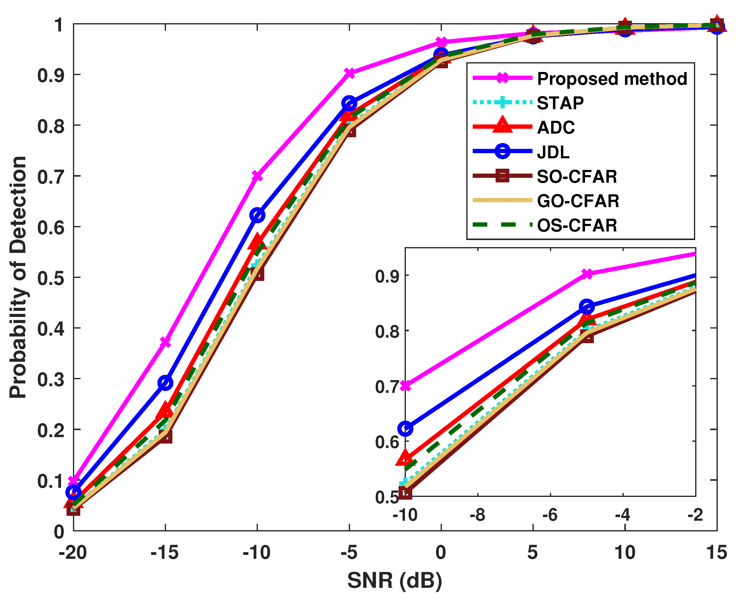
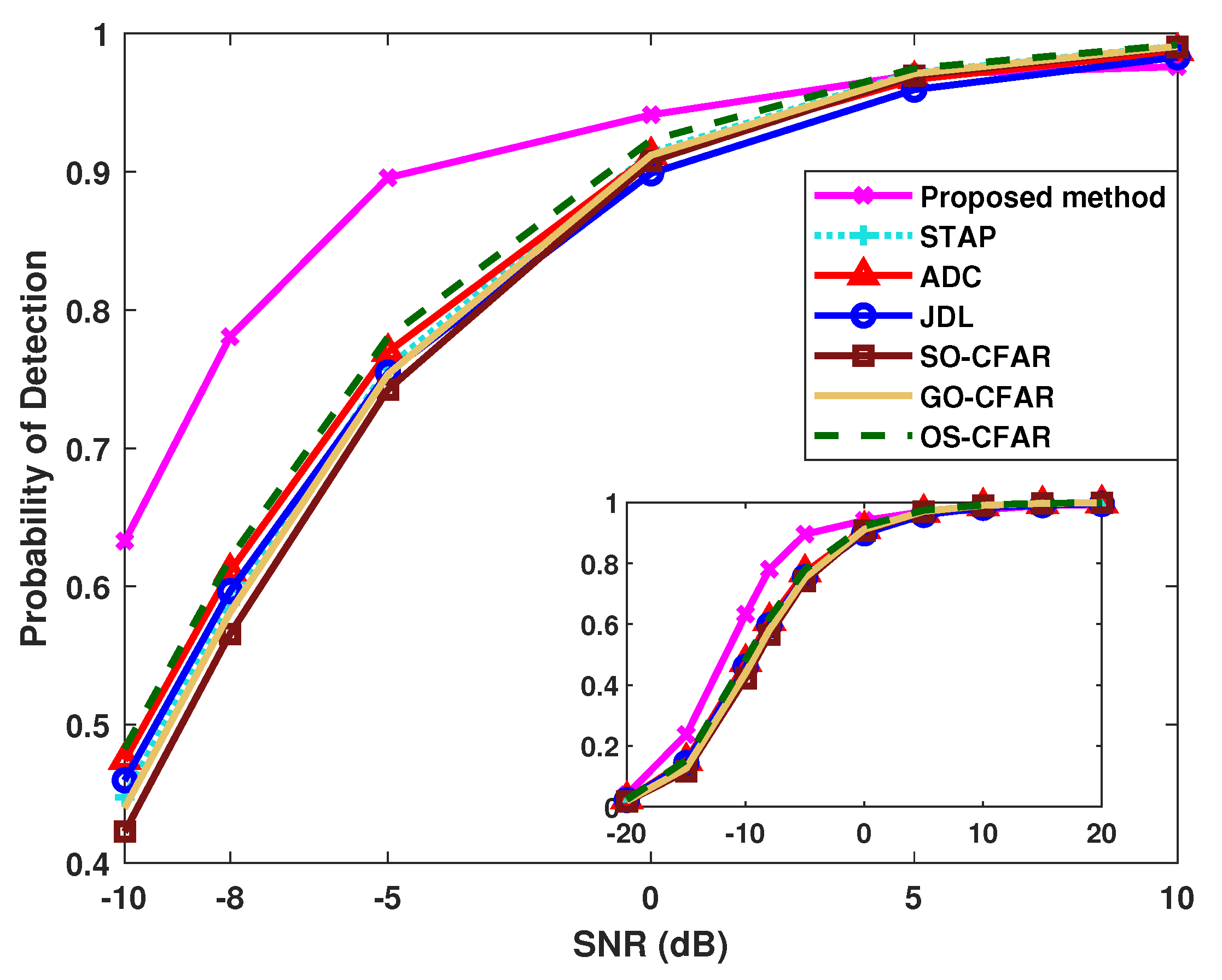
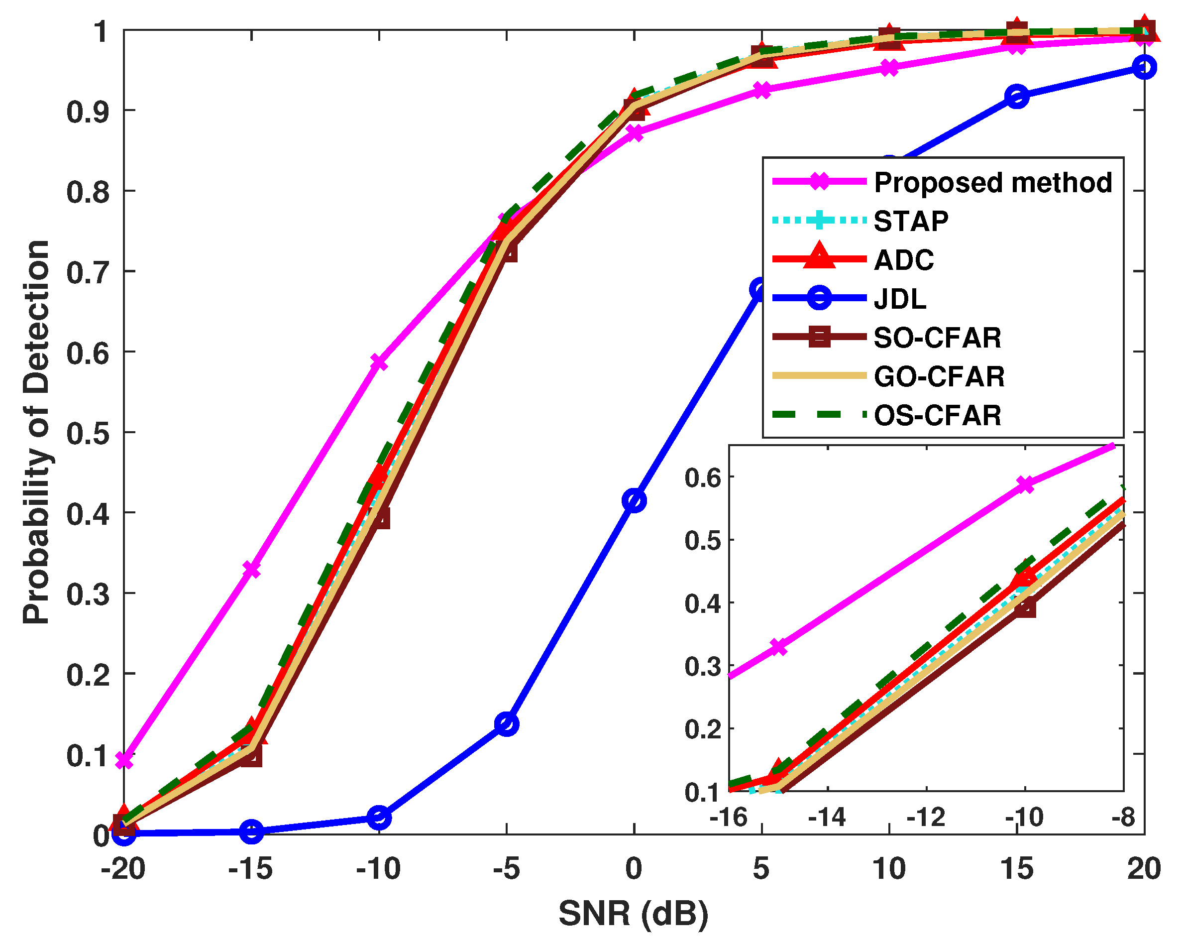
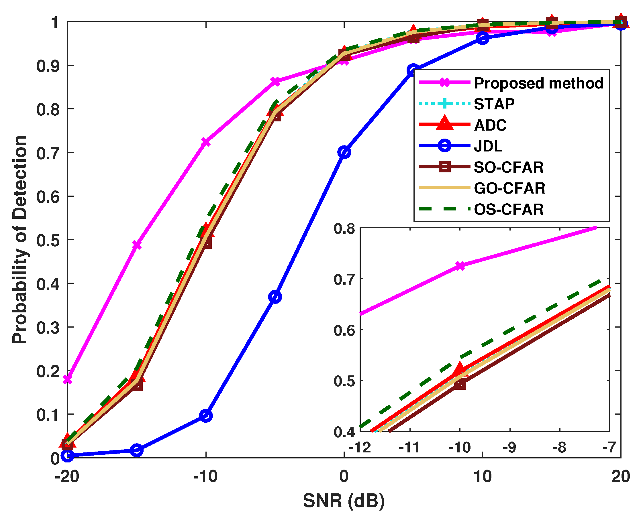
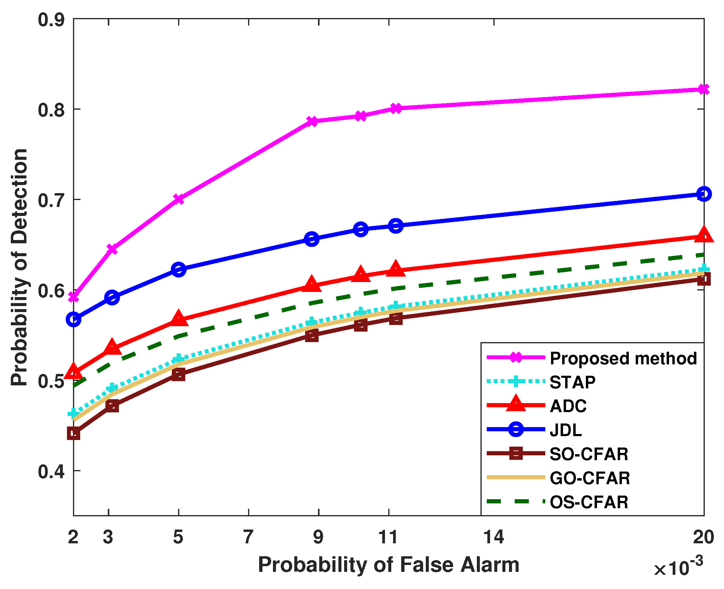
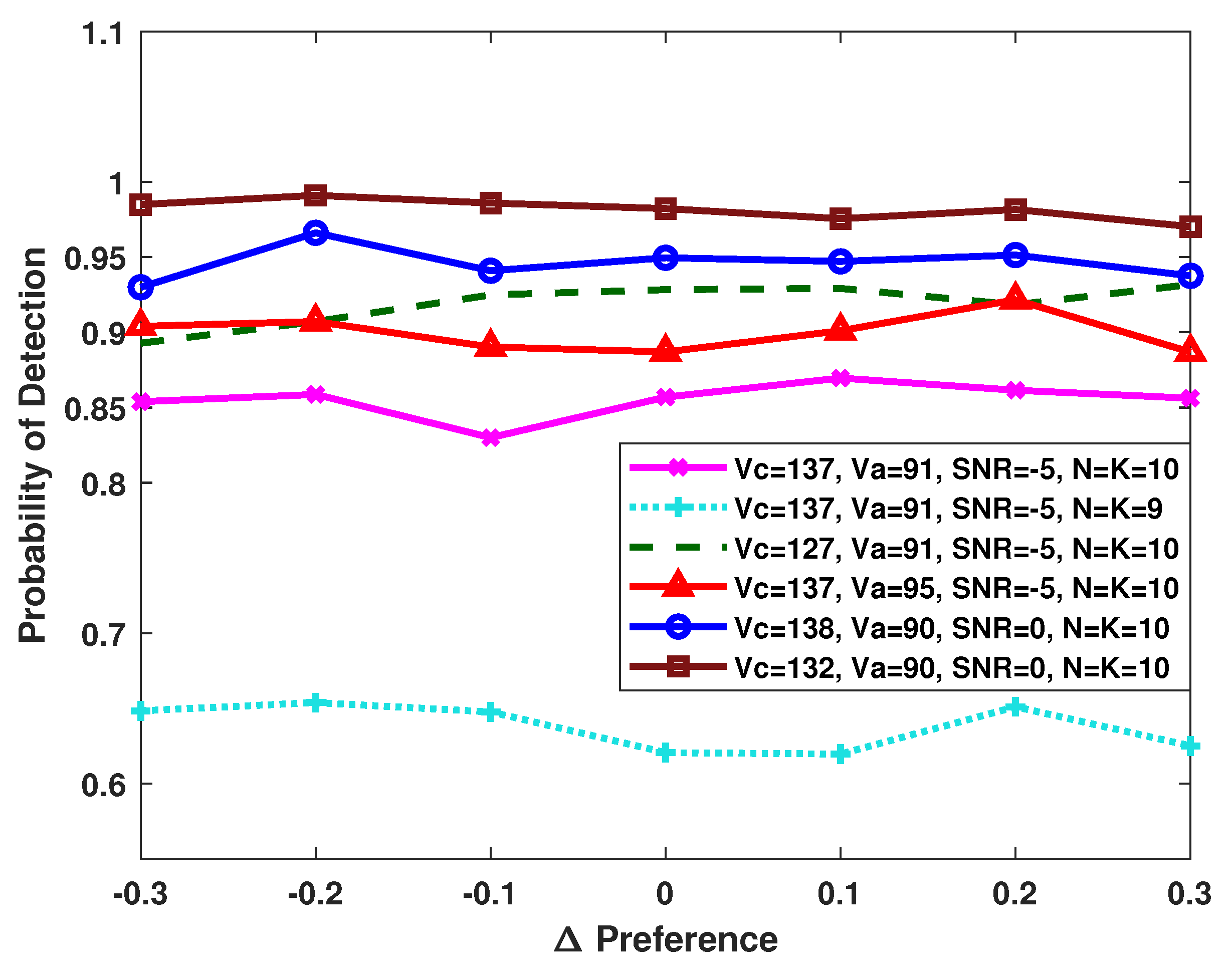
4.1. Results of the Probability of Detection

Figure 1 shows the performance of radar detection in clutter as a function of SNR. Radar is forward-looking, and its ϑ = 90 is known as the non-side-looking angle described before Equation (1). Moreover, the target azimuth velocity is v c = 138 m/s, and the airborne radar velocity is v a = 90 m/s. The collected samples from different cells are L = 60 in total, and it is assumed that the target is located at the ( L / 4 ) th range cell; meanwhile, CNR = 35 dB. The abbreviated PFA is used to express the probability of false alarms, which is set to be PFA = 5 × 10 3 for all the algorithms, including the proposed method. Specifically, we evaluate the STAP method [5], ADC method [13], JDL method [18], SO-CFAR method [23], GO-CFAR method [24] and OS-CFAR method [25]. The classical CA-CFAR method [22] is utilized for the target detection of the clutter suppression and range-compensation methods STAP, ADC and JDL. This simulation verifies that this proposed unsupervised method successfully suppresses the clutter in forward-looking radar. It overcomes the non-IID sample condition and the range dependence of clutter. It provides obviously better target detection performance than the other methods.
Figure 2 shows the radar-detection probabilities at various SNRs for different methods, under different conditions from Figure 1. We distinguish Figure 2 from Figure 1 by the fact that for Figure 2, the airborne radar velocity is v a = 91 m/s, the target azimuth velocity is v c = 137 m/s, CNR = 30 dB and the false alarm is PFA = 0.001 . The other circumstances are the same with those of Figure 1. In these conditions, OS-CFAR obtains slightly better detection than the other methods except for the proposed method. When the SNR is higher than about 12 dB, all of the detection algorithms can successfully realize the accurate detection of the moving target. Nevertheless, when the SNR is lower than about 10 dB, the proposed method achieves the highest probability of detection.
For further comparisons, a non-side-looking array with ϑ = 75 is used to show the detection with various SNRs in Figure 3. Furthermore, different v a = 100 m/s, v c = 130 m/s and CNR = 40 dB are used. PFA = 5 × 10 4 for all of the analyzed methods. In these simulation situations, the JDL method provides the lowest detection probability. With about 5 dB SNR 20 dB, the detection outcomes of STAP, ADC, SO-CFAR, GO-CFAR and OS-CFAR methods are good. However, when SNR is located at SNR = 20 to SNR = 5 dB, the proposed method performs the best.
To evaluate the influences of different situations, Figure 4 verifies the corresponding detection performance with various SNRs for the methods with a non-side-looking array whose ϑ = 25 ; meanwhile, v a = 80 m/s, v c = 130 m/s and CNR = 50 dB. For the proposed unsupervised algorithm, parameters are specified as u d 1 = 35 , u d 2 = 36 , u d 3 = 9 , u d 4 = 28 and u d 5 = 1 . The other conditions for the radar system and for the parameters are kept the same as those for Figure 1. From these results, we can analyze that the proposed unsupervised algorithm still maintains a distinct advantages in target detection over the other methods when SNR is below about SNR = 1 dB.
To visually show the target detected by different methods in Figure 4, space-time spectrum distributions without a target and with a target with respect to Figure 4 can be found in the upper subfigures of Figure 5. Additionally, the clutter and target distributions of the spectra corresponding to Figure 1 are also representatively depicted in the lower subfigures of Figure 5. Their respective SNRs are SNR = 20 dB and SNR = 30 dB. From the power spectra, we can analyze that broadened clutter ridges and targets make it difficult to achieve the target detection, especially in the low SNR region. However, in these conditions, the proposed unsupervised algorithm is effective. It performs well and is preferable to the other analyzed methods.
Figure 6 shows the comparison of different methods for the probability of detection with the variation in the probability of false alarm. The simulation conditions remain the same as those in Figure 1, except for the fixed SNR = 10 dB. The judgment intervals in the detection-discriminant criterion of the proposed method for radar detection are used to adjust the PFA. Specifically, the settings are { u d 2 = 8 and u d 3 = 12 } for PFA = 1.9 × 10 3 and { u d 2 = 8 } for PFA = 3.1 × 10 3 and { u d 2 = 10 } for PFA = 5 × 10 3 and { u d 1 = 7 } for PFA = 8.8 × 10 3 and { u d 1 = 6 } for PFA = 1.02 × 10 2 and { u d 1 = 6 , u d 5 = 40 45 } for PFA = 1.12 × 10 2 and { u d 1 = 1 , u d 5 = 50 } for PFA = 1.9 × 10 2 . For { u d i } i = 1 , 2 , 3 , 4 , 5 corresponding to each PFA, the other parameter settings that are not pointed out in particular stay the same as the parameters in Figure 1. With the same probabilities of false alarm mentioned above, the corresponding detection probabilities of the STAP, ADC, JDL, SO-CFAR, GO-CFAR and OS-CFAR methods are also evaluated. Figure 1 shows that increasing the PFA contributes to raising the detection probability for all of the methods. Moreover, the proposed method provides clear advantages over the other analyzed methods under different PFA conditions.

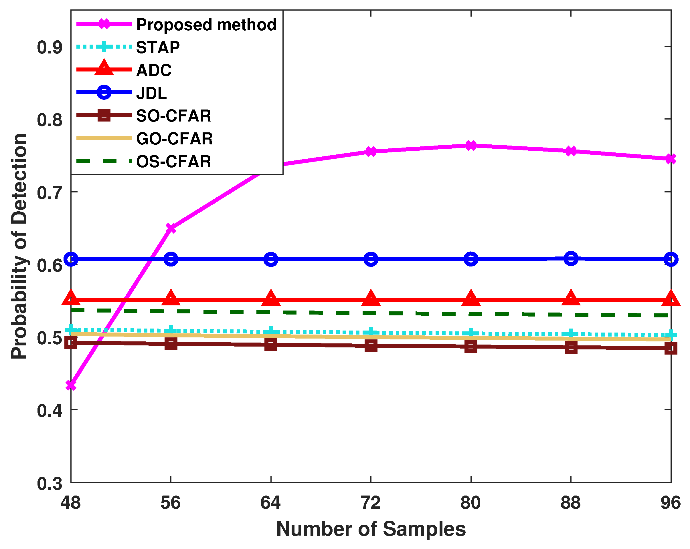
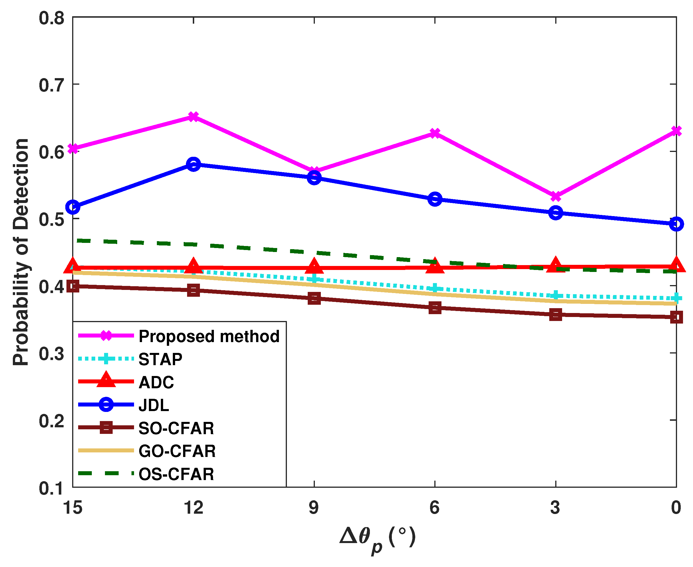
4.2. Influences of Sample Condition and Radar System Configuration

For evaluating different numbers of samples, Figure 7 reflects the comparison of detection probabilities with sample number variation at SNR = 10 dB, and the other conditions coincide with Figure 1. The number varies from L = 48 to L = 96 . It indicates that the range compensation method ADC for non-side-looking radar provides a higher probability of detection than STAP, JDL, SO-CFAR, GO-CFAR, and OS-CFAR methods. Furthermore, compared with those methods, JDL is superior in this situation. As the number grows gradually, the probability of detection rises to stability for the proposed method, which possess an apparent advantage over the others when the samples are more than about L = 54 . This is because the more exact power spectrum of clutter-plus-signal used to be the input for the proposed weighted clustering algorithm, contributes to more accurate numbers and centers of the clusters for the judgment of the designed detection-discriminant criterion.
The adaptation level of the proposed unsupervised algorithm for different ϑ of non-side-looking arrays is verified in Figure 8, where the non-side-looking angle described before Equation (1) is defined as ϑ = ( 90 + Δ θ p ) , and Δ θ p changes from Δ θ p = 0 to Δ θ p = 15 . In addition, SNR = 10 dB, PFA = 5 × 10 4 and the others are the same as those of Figure 1. For the proposed clustering algorithm, the changes of the radar system configurations cause different input data. Therefore, based on the original parameter settings, the parameters are adjusted to u d 1 = 8 Δ u , u d 2 = 10 Δ u , u d 3 = 11 Δ u , u d 4 = 30 Δ u and u d 5 = 42 Δ u , where Δ u = ceil { ( Δ θ p + 1 ) / 5 } 1 , with ceil { · } being an integer that is not less than { · } . From Figure 8, we can analyze that with the variations in ϑ , there are fluctuations in detection performance. For further improvement of the detection of the proposed method, more precise parameter settings can be introduced. However, on the whole, in Figure 8, the proposed unsupervised algorithm still performs far better than the others.

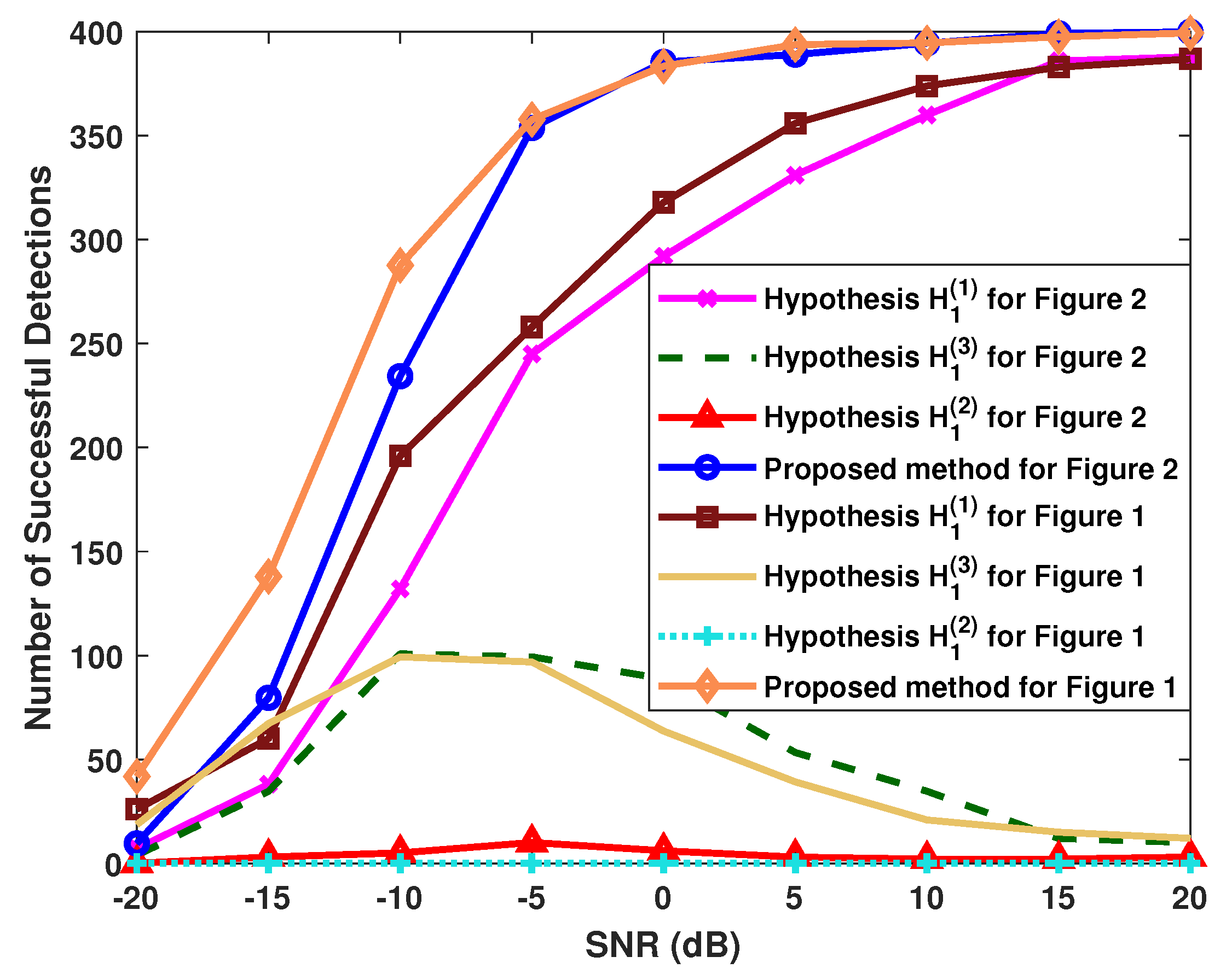
4.3. Influences of Parameters and Designed Hypotheses

Figure 9 evaluates the effects of the parameter settings of clustering preference p r e Y on detection probability for the proposed unsupervised algorithm, where preference is defined as p r e Y = 1.05 + Δ Preference with Δ Preference varying from Δ Preference = 0.3 to Δ Preference = 0.3 . The influences on different radar system configurations and moving target environments are considered. The differences in v c , v a , SNR , N and K for all the curves are indicated in Figure 9. It can be seen from Figure 9 that generally, as an empirical parameter, an appropriate setting of the preference can contribute to the desired performance of target detection. Furthermore, the setting of the clustering preference affects the probability of detection slightly, and the current settings in the proposed method are effective for all of the analyzed configurations and environments.
As the designed detection-discriminant criterion in the proposed method contains several hypotheses, including u d 1 to u d 5 and η 0 defined in Equation (33), their different contributions for accurate target detection are demonstrated. In this figure, { H 1 : x l = x c n , l + x s , l , when Q 1 = Q 2 = 1 , u d 1 I 1 Y u d 2 , u d 3 I 1 u d 4 } , { H 1 : x l = x c n , l + x s , l , when Q 1 = Q 2 = 1 , I 1 Y = u d 5 , u d 3 I 1 u d 4 } and { H 1 : x l = x c n , l + x s , l , when Q 1 = 1 , Q 2 = 2 , | x l | > η 0 } are briefly represented by the hypotheses H 1 ( 1 ) , H 1 ( 2 ) and H 1 ( 3 ) , respectively. Figure 10 reflects that the difference between the numbers Q 1 and Q 2 of the final formed clusters, that is, the designed H 1 ( 1 ) , contributes the most to accurate target detection. Especially at high SNR and SCR, this determines the vast majority of accurate detections. By contrast, a small percentage about one in eight of detections is provided from the hypothesis H 1 ( 3 ) . The one supplementary point u d 5 provides the least detections, and it can be flexibly adjusted with demand in different situations.

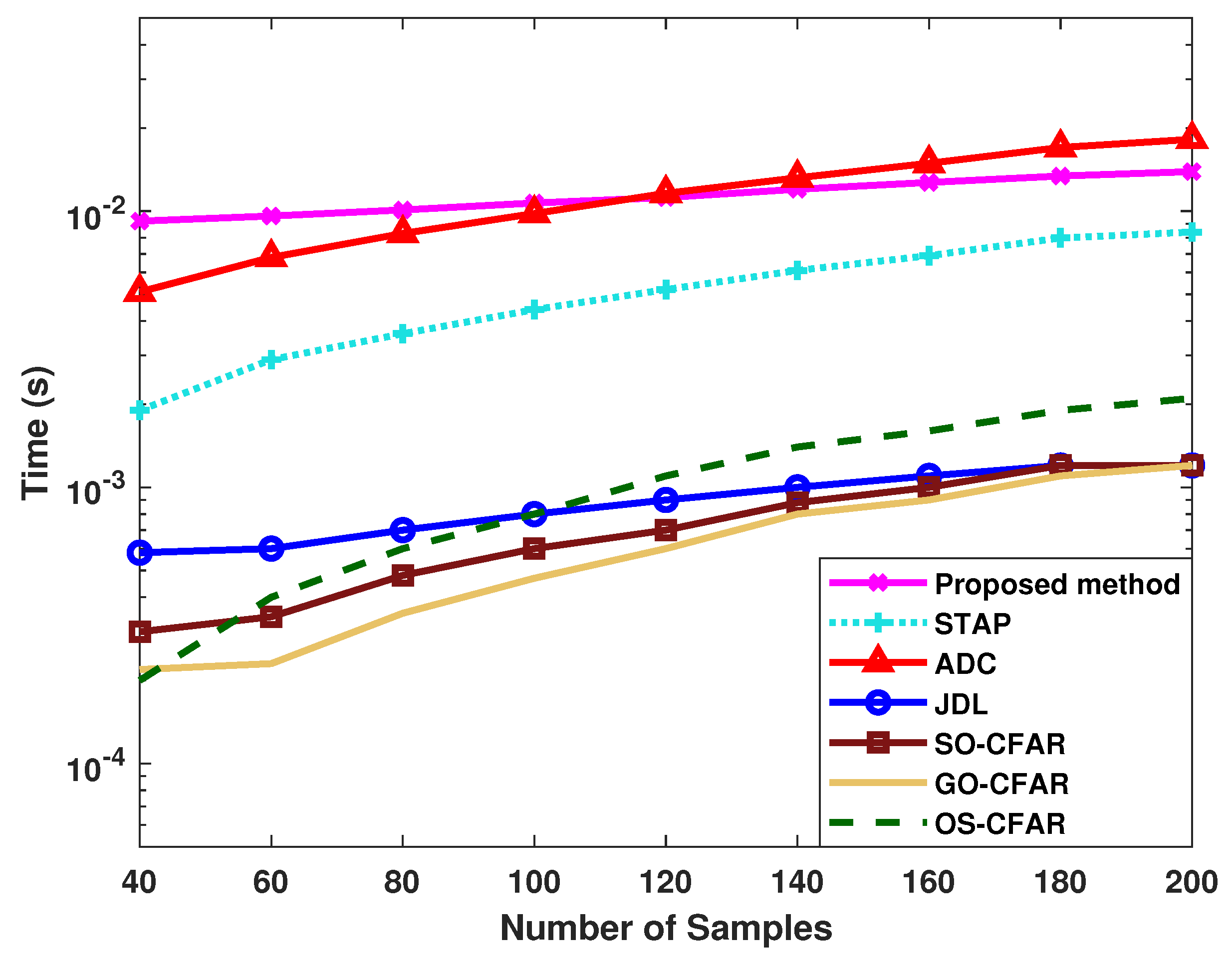
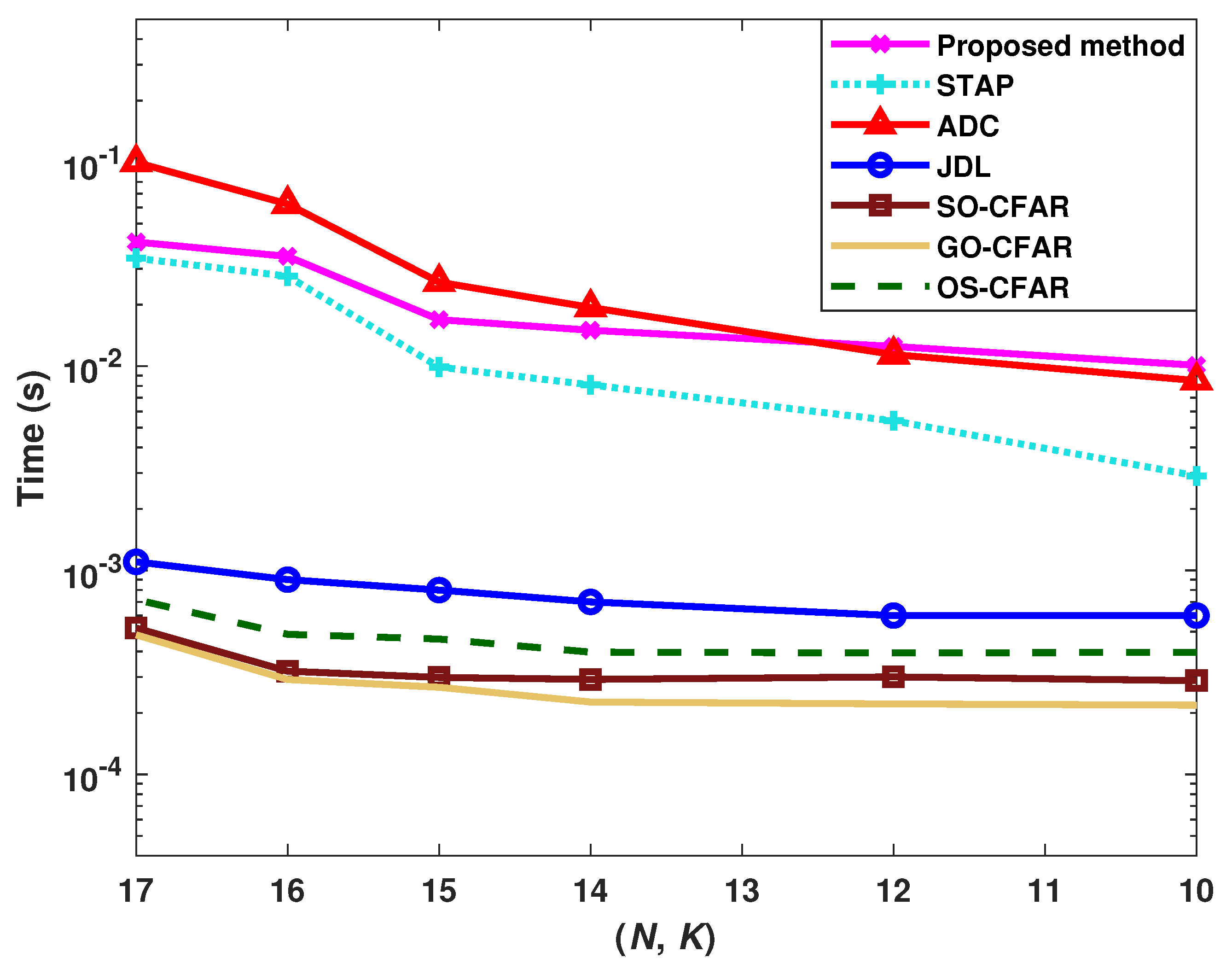
4.4. Computation Time of Different Methods

Figure 11 demonstrates the computation time versus different numbers L of training samples, and the conditions coincide with those in Figure 1. Various algorithms are included. The figure indicates that the computation time of JDL method, SO-CFAR method, GO-CFAR method and OS-CFAR method is relatively low. In contrast, the STAP method, the range compensation ADC method and the proposed method spend more time. The processes of ADC and the proposed unsupervised algorithm spend spend similar time when L is about L = 120 . With reasonable computation time, the proposed algorithm can achieve preferable performance in moving target detection.
Using various values of N and K, Figure 12 reflects the relationship between processing time and numbers of array elements and pules. Different methods are shown, and the conditions of Figure 1 are used with SNR = −10 dB. As N and K decrease, all the methods take less time. The processing of the proposed unsupervised algorithm requires less time than that of ADC when N and K are greater than about N = K = 12 , and its computation time is slightly greater than that of STAP. The computational complexity of the proposed method is about O { ( N K ) 3 + N 2 L + M 3 + [ M + 1 ( l s e 1 + l s e 2 ) ] 3 } , and the matrix sizes of the original received data and the designed clustering input data are the main factors that affect the computational complexity. As ADC makes pointed processing for the non-IID circumstance of the range dependence, and for this the proposed method proposes the unique design of distinguishing the two clustering processes, it is reasonable for them to have higher computational costs than STAP without compensation. The proposed unsupervised algorithm is obviously advantageous for its performance.

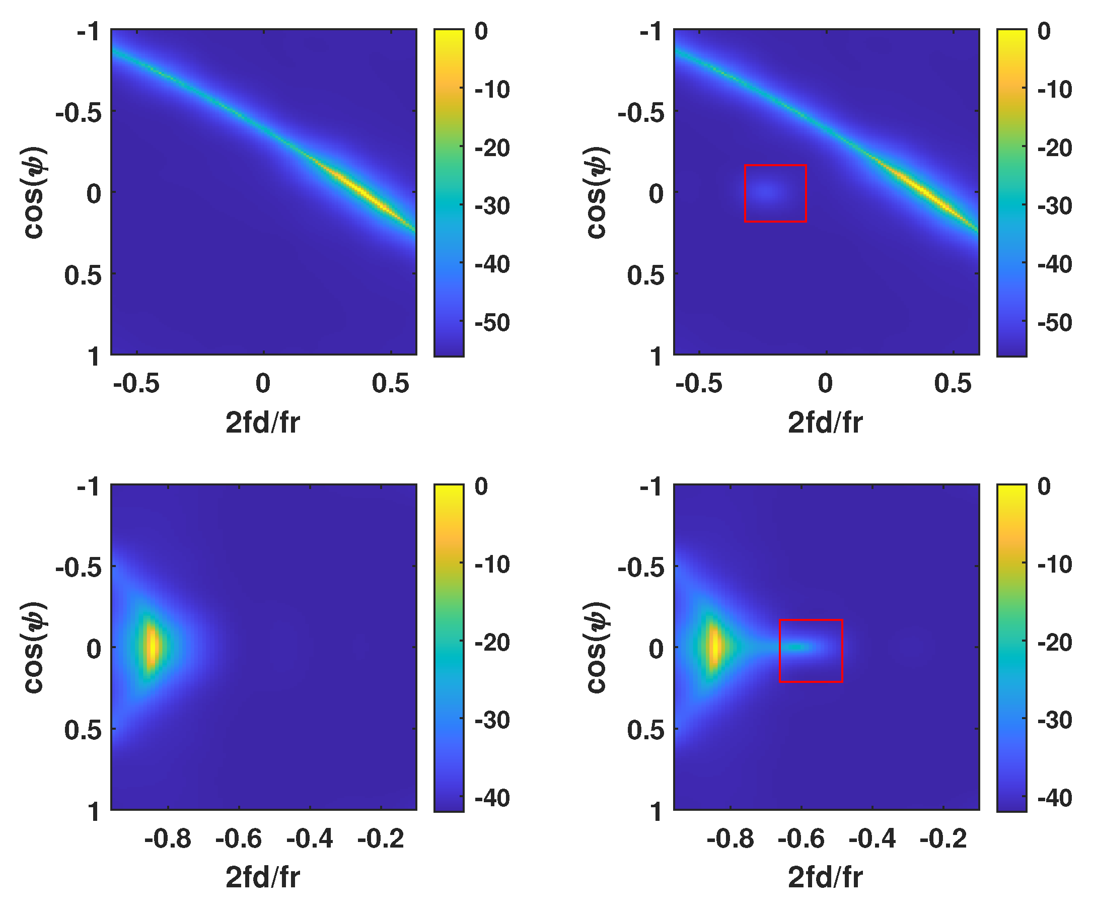
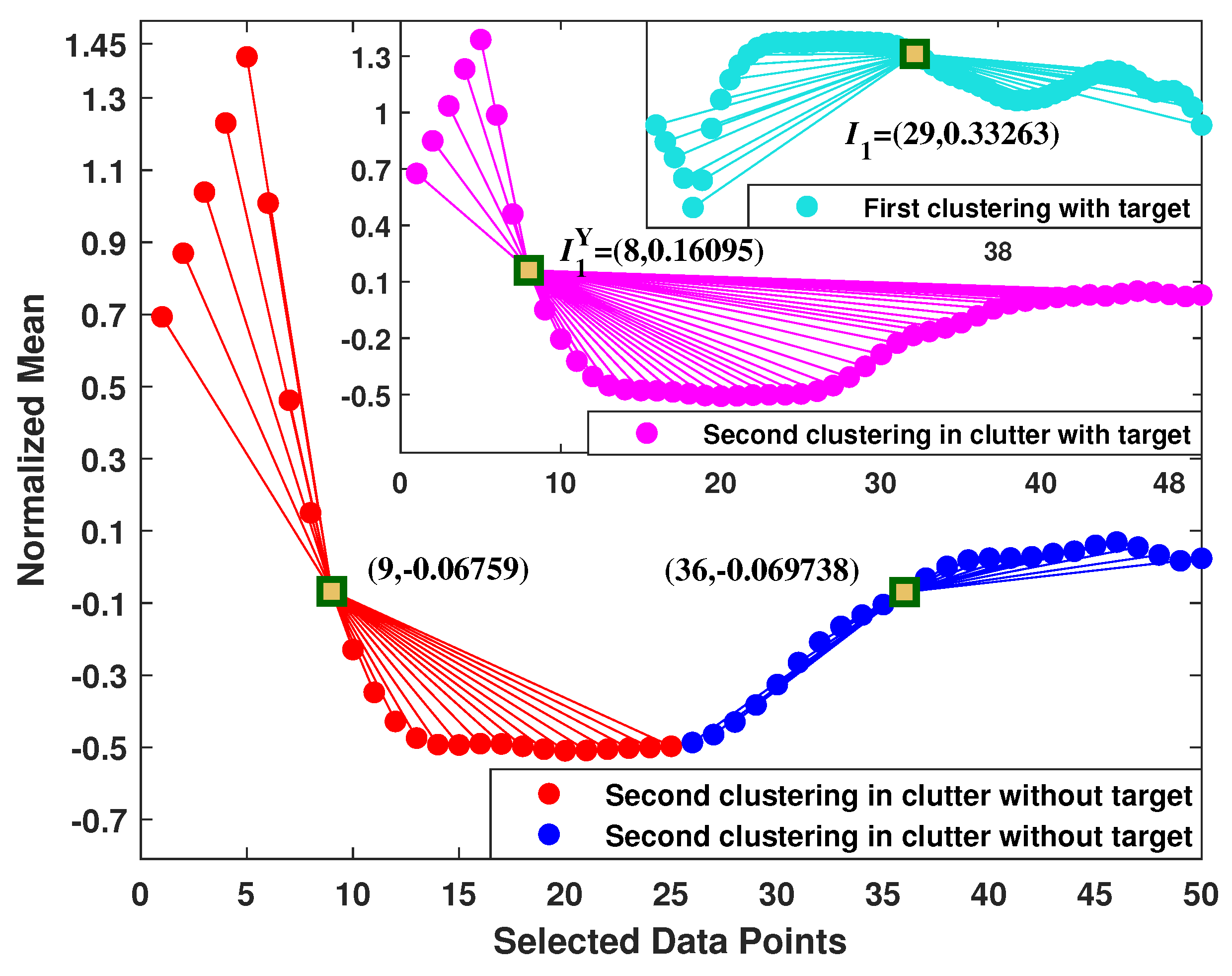
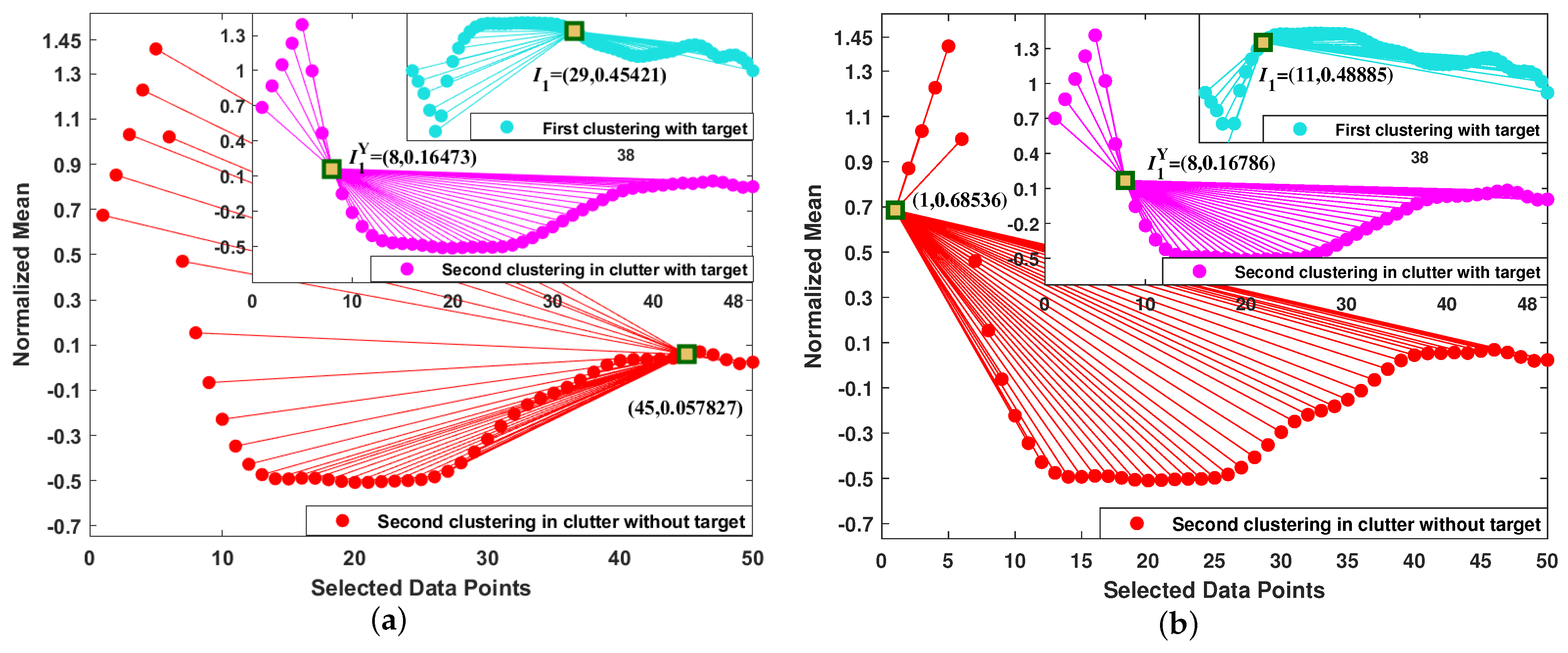
4.5. Visualization of the Formed Clusters

The clustering results are visually shown using the next simulation with visual data points. For directly representing different points, as a principal characteristic, the normalized mean value of the designed weighted input with respect to each range cell is brought in. The cluster centers are specially marked; meanwhile, their central locations with different horizontal and vertical coordinates are also indicated. SNR = 0 dB, and the other conditions coincide with Figure 2. Three circumstances of the designed second clustering containing the clutter without a target, the designed second clustering containing the clutter with a target, and the first clustering containing the clutter with a target, are considered for cluster visual comparison.
Without the target, the second clustering usually tends to split the points into two clusters, as seen in Figure 13, and the first clustering in this case provides one cluster, whose center is located at I 1 Y = ( 8 , 0.16095 ) . Figure 13 reflects that for the different circumstances mentioned above, the proposed detection clusterings can be distinguished from each other based on their numbers of final clusters, which are exploited for the designed detection-discriminant criterion.
There are only a few circumstances in which the second clustering in clutter without a target tends to produce one cluster, whose visualizations in various circumstances are shown in Figure 14a,b, where SNR = 0 dB. For the better cluster visualizations, Figure 13 and Figure 14 show one characteristic on the vertical axis. In fact, the proposed unsupervised algorithm fully excavates multiple potential characteristics used for target detection in clutter.
In Figure 14a, the only center for the second clustering in clutter without a target is I 1 Y = ( 45 , 0.057827 ) , whereas in Figure 14b, the center of the final formed cluster is I 1 Y = ( 1 , 0.68536 ) . In spite of the one cluster center occurring in the proposed second clustering under circumstance of target nonexistence, its center location is remote and and even near the size boundary of the selected data points. Therefore, it is not within the desired scope of locations proposed by the detection-discriminant criterion of Equation (33). Then, the circumstance in Figure 14 is determined as the target-nonexistence situation, along with the circumstance in Figure 13. Figure 14 reflects that for different circumstances, the proposed detection clusterings can be distinguished from each other based on their cluster centers, which are all exploited for the proposed detection discriminate criterion.

5. Discussion

Discussion 1: For parameters u d 1 to u d 5 in the detection-discriminant criterion, generally, a small interval of 1 u d 2 u d 1 4 can be considered, and u d 5 is regarded as the one supplementary point that may be another location of the cluster center. In addition, for the final weighted input matrix F ^ ˜ w designed from Equation (9) to Equation (13), if the changes of its dimension C M × L take place, u d 1 to u d 5 can be adjusted to desired target locations, which are not near the size boundary of the designed data point inputs F ^ ˜ w and Y ˜ w to be clustered. It is worth mentioning that with the same M, when constructing the power point matrix as the data input, unless major changes in the configurations happen, the empirical parameters u d 1 to u d 5 may remain unchanged for different radar system configurations and clutter-plus-noise environments, as demonstrated in the simulations.
Discussion 2: With regard to the numbers Q 1 and Q 2 of the final clusters and their respective cluster centers [ I 1 , I 2 , , I Q 2 ] and [ I 1 Y , I 2 Y , , I Q 2 Y ] , their analyses are as follows. In high proportions, there are two clusters with respective centers I 1 Y and I 2 Y for the second clustering of clutter without a target, whereas there is only one for the second clustering with a target. Although in a few cases, the second clustering without a target has one cluster center, its center location I 1 Y is remote and excluded from the proposed discriminate criterion for a target’s existence. As a consequence, unlike other radar detections, the proposed algorithm makes full use of clustering advantages, and its improved performance is well-founded and verifiable.
Discussion 3: Additionally, with respect to p r e and p r e Y involved in the preferences, to help to distinguish the differences between the two clustering processes for radar target detection, the preference adjustment parameter p r e Y for the designed second clustering can be a real number that is close to one, instead of being equal to one. In addition, by controlling the number of clusters, the aim of the first clustering is mainly finding an appropriate adjustment parameter p r e for the preference required by the proposed clusterings, which are specifically designed for radar data with clutter and target.

6. Conclusions

For non-side-looking airborne radar, an unsupervised AP clustering target detection algorithm is proposed, and simultaneously, it suppresses the clutter. The proposed unsupervised algorithm performs the designed unsupervised weighted AP clustering twice, with the corresponding constructed matrix-transformation based different weighted power inputs. Then, a detection-discriminant criterion based on the cluster results is further designed for the judgment of target detection, and simultaneously, the clutter is suppressed. With reasonable processing time, the proposed unsupervised algorithm achieves obviously higher probabilities of detection than the STAP, ADC, JDL, SO-CFAR, GO-CFAR and OS-CFAR algorithms. Moreover, it can better overcome the clutter-range dependence and better deal with the non-IID sample circumstances of non-side-looking radar than the others.

Author Contributions

Conceptualization, J.L. and G.L.; methodology, J.L.; software, J.L.; formal analysis, J.L. and F.H.J.; resources, J.L., G.L., C.Z. and J.X.; writing—original draft preparation, J.L.; writing—review and editing, J.L. and F.H.J.; project administration, J.L. and J.X.; funding acquisition, G.L., J.L., J.X., C.Z. and S.Z.; supervision, J.L. and F.H.J. All authors have read and agreed to the published version of the manuscript.

Funding

This work was supported by National Natural Science Foundation of China (NSFC) under grant 61901340, grant 61931016 and grant 62071344; the stabilization support of National Radar Signal Processing Laboratory under Grant KGJ20230X; and the Young Talent Starlet in Science and Technology in Shaanxi under No. 2022KJXX-38. In addition, it was supported by the Shaanxi Innovation Team 2022TD-38.

Data Availability Statement

Not applicable.

Conflicts of Interest

The authors declare no conflict of interest.

References

  1. Gong, M.G.; Cao, Y.; Wu, Q.D. A Neighborhood-Based Ratio Approach for Change Detection in SAR Images. IEEE Geosci. Remote Sens. Lett. 2012, 9, 307–311. [Google Scholar] [CrossRef]
  2. Kang, M.S.; Kim, K.T. Automatic SAR Image Registration via Tsallis Entropy and Iterative Search Process. IEEE Sens. J. 2020, 20, 7711–7720. [Google Scholar] [CrossRef]
  3. Hakim, W.L.; Achmad, A.R.; Eom, J.; Lee, C.W. Land Subsidence Measurement of Jakarta Coastal Area Using Time Series Interferometry with Sentinel-1 SAR Data. J. Coast. Res. 2020, 102, 75–81. [Google Scholar] [CrossRef]
  4. Ward, J. Space-Time Adaptive Processing for Airborne Radar; Technical Report; MIT Lincoln Laboratory: Lexington, KY, USA, 1998. [Google Scholar]
  5. Klemm, R. Principles of Space-Time Adaptive Processing; The Institution of Electrical Engineers: London, UK, 2002. [Google Scholar]
  6. Reed, I.S.; Mallett, J.D.; Brennan, L.E. Rapid convergence rate in adaptive arrays. IEEE Trans. Aerosp. Electron. Syst. 1974, AES-10, 853–863. [Google Scholar] [CrossRef]
  7. Lapierre, F.D.; Ries, P.; Verly, J.G. Foundation for mitigating range dependence in radar space-time adaptive processing. IET Radar Sonar Navig. 2009, 3, 18–29. [Google Scholar] [CrossRef] [Green Version]
  8. Lapierre, F.; Droogenbroeck, M.V.; Verly, J.G. New methods for handling the dependence of the clutter spectrum in non-sidelooking monostatic STAP radars. In Proceedings of the IEEE International Conference on Acoustics, Speech, and Signal Processing, Hong Kong, China, 6–10 April 2003; pp. 73–76. [Google Scholar]
  9. Lapierre, F.; Verly, J.G. Registration-based range dependence compensation for bistatic STAP radars. EURASIP J. Appl. Signal Process. 2005, 1, 85–98. [Google Scholar] [CrossRef] [Green Version]
  10. Lapierre, F.; Verly, J.G. Computationally-efficient range dependence compensation method for bistatic radar STAP. In Proceedings of the International Radar Conference, Arlington, VA, USA, 9–12 May 2005; pp. 714–719. [Google Scholar]
  11. Borsari, G.K. Mitigating effects on STAP processing caused by an inclined array. In Proceedings of the 1998 IEEE Radar Conference, Dallas, TX, USA, 12–13 May 1998; pp. 135–140. [Google Scholar]
  12. Kreyenkamp, O.; Klemm, R. Doppler compensation in forward-looking STAP radar. IEEE Proc. Radar Sonar Navig. 2001, 148, 253–258. [Google Scholar] [CrossRef]
  13. Himed, B.; Zhang, Y.; Hajjari, A. STAP with angle-Doppler compensation for bistatic airborne radars. In Proceedings of the IEEE Radar Conference, Long Beach, CA, USA, 22–25 April 2002; pp. 311–317. [Google Scholar]
  14. Pearson, F.; Borsari, G. Simulation and analysis of adaptive interference suppression for bistatic surveillance radars. In Proceedings of the Adaptive Sensor Array Process; LincoIn Laboratory: VIrkshop, MA, USA, 2001. [Google Scholar]
  15. Guerci, J.R.; Goldstein, J.S.; Reed, I.S. Optimal and adaptive reduced-rank STAP. IEEE Trans. Aerosp. Electron. Syst. 2000, 36, 647–663. [Google Scholar] [CrossRef]
  16. Liao, G.S.; Bao, Z.; Xu, Z.Y. A framework of rank-reduced space-time adaptive processing for airborne radar and its applications. Sci. China Ser. Technol. Sci. 1997, 40, 505–512. [Google Scholar] [CrossRef]
  17. Goldstein, J.S. Reduced rank adaptive filtering. IEEE Trans. Signal Process 1997, 45, 492–496. [Google Scholar] [CrossRef]
  18. Wang, Y.; Peng, Y. Space-time joint processing method for simultaneous clutter and jamming rejection in airborne radar. Electron. Lett. 1996, 32, 258. [Google Scholar] [CrossRef]
  19. Wang, W.L.; Liao, G.S.; Zhang, G.B. Improvement on the performance of the auxiliary channel STAP in the non-homogeneous environment. J. Xidian Univ. 2004, 20, 426–429. [Google Scholar]
  20. Gini, F.; Greco, M. Covariance matrix estimation for CFAR detection in correlated heavy tailed clutter. Signal Process. 2002, 82, 1847–1859. [Google Scholar] [CrossRef]
  21. Hammoudi, Z.; Soltani, F. Distributed CA-CFAR and OS-CFAR detection using fuzzy spaces and fuzzy fusion rules. IEE Proc.-Radar Sonar Navig. 2004, 15, 135–142. [Google Scholar] [CrossRef]
  22. Zaimbashi, A. An adaptive cell averaging-based CFAR detector for interfering targets and clutter-edge situations. Digit. Signal Process. 2014, 31, 59–68. [Google Scholar] [CrossRef]
  23. Trunk, G.V. Range resolution of targets using automatic detectors. IEEE Trans. Aerosp. Electron. Syst. 1978, 14, 750–755. [Google Scholar] [CrossRef]
  24. Gandhi, P.; Kassam, S. Analysis of CFAR processors in nonhomogeneous background. IEEE Trans. Aerosp. Electron. Syst. 1988, 24, 427–445. [Google Scholar] [CrossRef]
  25. Rohling, H. Radar CFAR thresholding in clutter and multiple target situations. IEEE Trans. Aerosp. Electron. Syst. 1983, 19, 608–621. [Google Scholar] [CrossRef]
  26. Wang, P.; Li, H.; Himed, B. A New Parametric GLRT for Multichannel Adaptive Signal Detection. IEEE Trans. Signal Process. 2010, 58, 317–325. [Google Scholar] [CrossRef]
  27. Liu, W.J.; Liu, J.; Hao, C.P.; Gao, Y.C.; Wang, Y.L. Multichannel adaptive signal detection: Basic theory and literature review. Sci. China Inf. Sci. 2022, 65, 121301. [Google Scholar] [CrossRef]
  28. Shi, B.; Hao, C.P.; Hou, C.H.; Ma, X.C.; Peng, C.Y. Parametric Rao test for multichannel adaptive detection of range-spread target in partially homogeneous environments. Signal Process. 2015, 108, 421–429. [Google Scholar] [CrossRef]
  29. Liao, L.Y.; Du, L.; Guo, Y.C. Semi-supervised SAR target detection based on an improved faster R-CNN. Remote Sens. 2022, 14, 143. [Google Scholar] [CrossRef]
  30. Zhang, F.; Du, B.; Zhang, L.; Xu, M. Weakly Supervised Learning Based on Coupled Convolutional Neural Networks for Aircraft Detection. IEEE Trans. Geosci. Remote Sens. 2016, 54, 5553–5563. [Google Scholar] [CrossRef]
  31. Frey, B.J.; Dueck, D. Clustering by passing messages between data points. Science 2007, 315, 972–976. [Google Scholar] [CrossRef] [Green Version]
  32. Wang, K.; Zhang, J.; Li, D.; Zhang, X.; Guo, T. Adaptive affinity propagation clustering. Acta Autom. Sin. 2007, 33, 1242–1246. [Google Scholar]
  33. Liu, J.; Liao, G.S.; Xu, J.W.; Zhu, S.Q.; Juwono, F.J.; Zeng, C. Autoencoder neural network-based STAP algorithm for airborne radar with inadequate training samples. Remote Sens. 2022, 14, 6021. [Google Scholar] [CrossRef]
  34. Zou, B.; Wang, X.; Feng, W.; Zhu, H.; Lu, F. DU-CG-STAP method based on sparse recovery and unsupervised learning for airborne radar clutter suppression. Remote Sens. 2022, 14, 3472. [Google Scholar] [CrossRef]
  35. Duan, K.; Chen, H.; Xie, W.; Wang, Y. Deep learning for high-resolution estimation of clutter angle-Doppler spectrum in STAP. IET Radar Sonar Navig. 2022, 16, 193–207. [Google Scholar] [CrossRef]
  36. Zhu, H.; Feng, W.; Feng, C.; Zou, B.; Lu, F. Deep Unfolding Based Space-Time Adaptive Processing Method for Airborne Radar. J. Radars 2022, 11, 1–16. [Google Scholar]
  37. Xu, J.W.; Liao, G.S.; Huang, L.; Zhu, S.Q. Joint magnitude and phase constrained STAP approach. Digital Signal Process. 2015, 46, 32–40. [Google Scholar] [CrossRef]
  38. Cui, W.; Wang, T.; Wang, D.; Liu, C. An improved iterative reweighted STAP algorithm for airborne radar. Remote Sens. 2023, 15, 130. [Google Scholar] [CrossRef]
  39. Wang, D.; Wang, T.; Cui, W.; Liu, C. Adaptive support-driven sparse recovery STAP method with subspace penalty. Remote Sens. 2022, 14, 4463. [Google Scholar] [CrossRef]
  40. Ottersten, B.; Stoica, P.; Roy, R. Covariance matching estimation techniques for array signal processing applications. Digital Signal Process. 1998, 8, 185–210. [Google Scholar] [CrossRef]
Figure 1. Comparison of detection probabilities with various SNRs.
Remotesensing 15 02077 g001
Figure 2. Comparison of detection probabilities with various SNRs.
Remotesensing 15 02077 g002
Figure 3. Relationship between PD and SNR.
Remotesensing 15 02077 g003
Figure 4. Relationship between PD and SNR.
Remotesensing 15 02077 g004
Figure 5. Space-time spectrum distributions of clutter without a target (left column) and with the target (right column).
Remotesensing 15 02077 g005
Figure 6. Probability of detection versus probability of false alarm for different methods.
Remotesensing 15 02077 g006
Figure 7. PD with variation in the number of training samples.
Remotesensing 15 02077 g007
Figure 8. Probability of detection versus non-side-looking angle for different methods.
Remotesensing 15 02077 g008
Figure 9. Probability of detection versus different clustering preferences.
Remotesensing 15 02077 g009
Figure 10. Comparison of the contributions of different hypotheses.
Remotesensing 15 02077 g010
Figure 11. Relationship between computation time and number of samples.
Remotesensing 15 02077 g011
Figure 12. Computation time versus numbers of array elements and pules (N and K).
Remotesensing 15 02077 g012
Figure 13. Visualization of the formed clusters when Q 2 = 2 .
Remotesensing 15 02077 g013
Figure 14. Visualizations of the formed clusters when Q 2 = 1 . (a) I 1 Y = ( 45 , 0.057827 ) in clutter without a target. (b) I 1 Y = ( 1 , 0.68536 ) in clutter without a target.
Remotesensing 15 02077 g014
Table 1. The processing procedure of the proposed unsupervised algorithm.
1.
After the matched filtering, the stacked vector with K pulses composes the received radar data as seen in Equation (4).
2.
On the basis of the power characteristics of clutter plus noise and signal, matrix transformation based weighted input data matrix F ^ ˜ w is proposed.
(a)
The power data points are selected as Equation (9), and the STAP weight vector is calculated from Equation (6);
(b)
A series of matrix transformations, are proposed as Equations (10)–(13).
3.
Exploiting the designed F ^ ˜ w , the proposed method performs the first unsupervised weighted AP clustering by means of similarity s ( i , j ) , responsibility ( i , j ) and availability β ( i , j ) for 1 i , j M .
(a)
The similarity of any two points is obtained from Equations (14) and (15);
(b)
The preference for the clustering is designed as Equation (16);
(c)
The responsibility and availability are updated by Equations (18)–(25), until the number of the final clusters Q 1 and the corresponding cluster centers [ I 1 , I 2 , , I Q 1 ] are obtained.
4.
New reconstructed weighted power inputs Y ˜ w are proposed as Equation (29).
5.
The proposed method further designs the second unsupervised weighted AP clustering denoted as Equation (31), with the new designed preference in Equation (32). Therefore, the number of the final clusters Q 2 and the corresponding cluster centers [ I 1 Y , I 2 Y , , I Q 2 Y ] are obtained.
6.
With their cluster results, a detection-discriminant criterion is designed for the judgement of target detection as Equation (33).
Disclaimer/Publisher’s Note: The statements, opinions and data contained in all publications are solely those of the individual author(s) and contributor(s) and not of MDPI and/or the editor(s). MDPI and/or the editor(s) disclaim responsibility for any injury to people or property resulting from any ideas, methods, instructions or products referred to in the content.

