Article

Global Mangrove Watch: Monthly Alerts of Mangrove Loss for Africa

1
Department Geography and Earth Sciences, Aberystwyth University, Aberystwyth SY23 3DB, UK
2
Wetlands International, 6700 AL Wageningen, The Netherlands
3
solo Earth Observation (soloEO), Tokyo 104-0054, Japan
4
Wetlands International Eastern Africa, Nairobi PQ7X+5J7, Kenya
5
Wetlands International West Africa, Dakar MGXW+333, Senegal
*
Author to whom correspondence should be addressed.
Remote Sens. 2023, 15(8), 2050; https://doi.org/10.3390/rs15082050
Submission received: 30 January 2023 / Revised: 30 March 2023 / Accepted: 6 April 2023 / Published: 12 April 2023
(This article belongs to the Special Issue Remote Sensing in Mangroves III)

Abstract

:
Current mangrove mapping efforts, such as the Global Mangrove Watch (GMW), have focused on providing one-off or annual maps of mangrove forests, while such maps may be most useful for reporting regional, national and sub-national extent of mangrove forests, they may be of more limited use for the day-to-day management of mangroves and for supporting the Global Mangrove Alliance (GMA) goal of halting global mangrove loss. To this end, a prototype change mangrove loss alert system has been developed to identify mangrove losses on a monthly basis. Implemented on the Microsoft Planetary Computer, the Global Mangrove Watch v3.0 mangrove baseline extent map for 2018 was refined and used to define the mangrove extent mask under which potential losses would be identified. The study period was from 2018 to 2022 due to the availability of Sentinel-2 imagery used for the study. The mangrove loss alert system is based on optimised normalised difference vegetation index (NDVI) thresholds used to identify mangrove losses and a temporal scoring system to filter false positives. The mangrove loss alert system was found to have an estimated overall accuracy of 92.1%, with the alert commission and omission estimated to be 10.4% and 20.6%, respectively. Africa was selected for the mangrove loss alert system prototype, where significant losses were identified in the study period, with 90% of the mangrove loss alerts identified in Nigeria, Guinea-Bissau, Madagascar, Mozambique and Guinea. The primary drivers of these losses ranged from economic activities that dominated West Africa and Northern East Africa (mainly agricultural conversion and infrastructure development) to climatic in Southern East Africa (primarily storm frequency and intensity). The production of the monthly mangrove loss alerts for Africa will be continued as part of the wider Global Mangrove Watch project, and the spatial coverage is expected to be expanded to other regions over the coming months and years. The mangrove loss alerts will be published on the Global Mangrove Watch online portal and updated monthly.

Graphical Abstract

1. Introduction

Mangroves are a globally important [1] and dynamic [2] ecosystem providing a range of ecosystem services, including blue carbon [3,4], biodiversity [5], fisheries [6], coastal protection [7,8], and tourism [9]. Mangroves are an ecosystem under pressure [10,11] with significant losses occurring since the 1980s [12,13]. The Global Mangrove Alliance (GMA [14]) has set the goals of halting mangrove loss, increasing the amount of mangrove restoration and increasing mangrove protection through building awareness.
The Global Mangrove Watch (GMW) mangrove extent layers [15,16,17,18] cover eleven annual epochs between 1996 and 2020, and provide the most up to date historical extents of mangroves globally. They are available through the Global Mangrove Watch online Portal [19]. However, given their annual update cycle, these layers may be of limited use for users looking to manage regions and protected areas containing mangrove forests. For efficient protection from human activities and informing on natural events disrupting mangroves, losses need to be identified as close to the loss event as possible and provided to users in a form they can easily use.
The GMW Portal [19] is subject to ongoing development, with additional functionality and improvements to hosted datasets being added at regular intervals. For example, an early version of the mangrove loss alerts was provided when the portal launched in July 2021 and has subsequently been updated with the results of this study in February 2023. This enables users without technical GIS or remote sensing skills to access and analyse mangrove loss alerts in near-real time. Users of the GMW datasets and the GMW Portal fall into several categories, including those who (a) seek a national or regional view of mangrove changes, with these tending to be academic or policy users, and (b) are tasked with managing and protecting small regions of mangroves (e.g., a national park, a single delta or section of coastline). Practitioners focused on small regions of mangroves would commonly have significant knowledge of the area in which they work. Therefore, global maps of annual mangrove changes may be of limited use. However, regularly visiting all parts of their area of interest is often not feasible. Therefore, being alerted to mangrove losses that have recently occurred can be useful, even if identifying illegal or unintended losses that could be stopped if caught in time.
For the reasons outlined above, the GMW Mangrove Loss Alerts were developed to provide a system for mapping mangrove losses in a timely manner, such that information can be provided to users allowing them to act accordingly [20]. To achieve this aim, the following objectives were identified for the system proposed within this article:
  • Provide updates at least monthly, thereby allowing end users to respond to ongoing activities or be informed of natural events that compromise the integrity or existence of mangroves.
  • Provide a low number of false positives; alerts might be ignored if false alerts are generated regularly.
  • Provide a basis for an operational system; implemented in a suitable computing platform with a maintainable code base.
  • To be computationally viable to scale to mangrove regions globally.
Africa was selected for prototype development and validation of the GMW Mangrove Loss Alerts system as it is a geographically discrete continent and sufficiently large in area to test scalability. It also comprises a range of mangrove types and conditions with areas, such as the Niger Delta known to have significant ongoing changes. There is significant variability between western and eastern Africa in terms of cloud cover and climate, with East Africa typically drier [21] and the South East witnessing a number of cyclones each year. Areas of West Africa are often characterised by significant cloud cover, allowing any limitations in the use of optical satellite data due to cloud cover to be identified. Finally, through GMA partners, such as Wetlands International, local knowledge of many regions could be collected and fed into optimising and validating the system. The monthly GMW Mangrove Loss Alerts dataset is available to users through the Global Mangrove Watch online Portal [19]. The version available on the GMW Portal was updated with the results of this study in February 2023 and will be updated on a monthly basis going forward.

2. Background

Many studies (e.g., [2,15,22,23,24]) have considered mapping land cover change, including forest loss, through remote sensing imagery using various sensors, modalities and methods. There are a number of approaches to mapping land cover change, but these fit within four broad categories, (1) map-to-map, (2) image-to-image, (3) map-to-image and (4) time series approaches. Map-to-map approaches (e.g., [25]) detect change by producing two or more classifications and comparing the resulting categorical maps. The advantages of such approaches are that they are independent of the datasets used to derive the maps, and therefore, different modalities can be used and compared. However, they can also find false positives due to errors within the classifications. Image-to-image approaches (e.g., [26]) require no supplementary data, such as a map and/or training data, but the imagery does need to be comparable. However, it is common for changes in image pixel values to not necessarily relate to a change in land cover but to changes in the season and/or condition of the land cover. Map-to-image approaches (e.g., [15]) require that each class has a defined response (e.g., reflectance or backscatter) within the remotely sensed imagery and that a change in land cover will cause that response to change such that it is identifiably different from the original class. These approaches often merge the advantages of the map-to-map and image-to-image approaches while mitigating many of the negatives. Time series approaches (e.g., [27,28,29,30]) model each pixel within a scene, either mapping the trend of each pixel or allowing the future pixel responses to be predicted and therefore compared to the observed response. A significant difference between the observed and predicted or the slope for the trend crossing a predetermined threshold allows for a change to be identified. These methodologies allow for seasonality and natural variations in response to be taken into account, thereby reducing the number of false positives for changes. Additionally, these methodologies can also assess long-term trends in response, providing the possibility for condition-based changes to be mapped (e.g., [31]). However, time series approaches are computationally expensive, requiring significant computational resources to fit the models and predict further observations. Computational costs can be reduced by reducing the frequency in which the models are re-fitted, such as re-fitting monthly or quarterly rather than after each observation. However, this can reduce the accuracy of the modelling approach.
There are two systems which provide publicly available forest loss alerts. The Global Forest Watch (GFW) alerts are provided from a combination of Global Land Analysis and Discovery lab (GLAD; [32]) and radar for detecting deforestation (RADD; [33]) systems. The Japan International Cooperation Agency (JICA) and Japan Aerospace Exploration Agency (JAXA) provide the JICA-JAXA Forest Early Warning System (JJ-FAST; [34]) alerts. While other systems have been proposed (e.g., [35,36]), many are based on lower spatial resolution datasets, such as MODIS, and/or have provided alerts for a specific country and therefore are not directly relevant to this study.
The GLAD alerts [32] are derived from USGS Landsat imagery with a pixel resolution of 30 m. A bagged tree machine learning classification algorithm is used and applied to each scene to identify possible areas of change. The system confirms a change if at least two from four consecutive scenes identify a pixel as a change. For a case study in Peru, the users accuracy was estimated at 86.5% ± 2.0 (13.5% commission) and producers as 67.0% ± 7.4 (33.0% omission).
The RADD [33] system uses Copernicus Sentinel-1 C-band SAR imagery with a spatial pixel resolution of 10 m and an updated period of 6–12 days. Although, with the failure of Sentinel-1B in December 2021, the RADD system is limited until the launch of Sentinel-1C, expected in 2023. The Sentinel-1 VH and VV backscatter are converted into per-pixel forest and non-forest probabilities using historical Gaussian mixture models. A non-forest threshold is then used to identify forest loss alerts, and Bayesian updating is applied to confirm alerts using subsequent observations. Using a case study from the Congo Basin, the users and producers accuracies were estimated as 97.6% (2.4% commission) and 95.0% (5% omission), respectively.
The JJ-FAST system [34] uses JAXA ALOS-2/PALSAR-2 ScanSAR L-band SAR data to provide deforestation alerts for 77 countries every 42 days with a spatial pixel resolution of 50 m. The approach has evolved with a number of versions of the algorithm released, all based on a system of thresholds. A number of global reference sites were used to define the thresholds. The users and producers accuracies for Version-3 of the alerts were estimated at 85.0% (15% commission) and 63.8% (36.2% omission), respectively.
The system proposed by this study used a map-to-image approach to identify mangrove loss alerts. A refined version of the GMW 2018 mangrove extent was used to define the mangrove extent, and a computationally simple normalised difference vegetation index (NDVI)-based threshold methodology was developed to identify the mangrove loss alerts on a monthly basis. Our system has similarities to the JJ-FAST approach in that a set of optimised thresholds are used to define change, rather than a machine learning-based classification or modelling approach. However, it is also similar to the GLAD alerts system as the proposed system uses multiple observations to confirm a change.

3. Methods

The analysis for the GMW Mangrove Loss Alerts was undertaken via the Microsoft Planetary Computer [37,38], which provides access to the many spatial datasets, including the full Sentinel-2 archive, hosted within an Azure storage bucket and searchable via a STAC API [39]. Using the freely provided jupyter-lab [40] Kubernetes [41] deployment, the Microsoft Planetary Computer allows access to a Dask [42] cluster to scale data analysis. For this study, the items identified through the STAC search API were loaded as a Xarray [43] into the Dask [42] cluster using the Open Data Cube (ODC) STAC API [44]. In the future, when computer requirements go beyond those provided in the free Kubernetes deployment, scaling can be achieved through the deployment of a custom Kubernetes deployment within the Microsoft Azure Cloud.
Analysis was undertaken on a 1 × 1 degree grid (Figure 1) with all data resampled into the WGS84 (EPSG:4326) coordinate system. A pixel size of 0.0002 degrees (∼22 m) was used, resulting in output images for each 1 × 1 degree tile of 5000 × 5000 pixels. Therefore, each mangrove loss alert point represents a 0.0002 × 0.0002 degree pixel (i.e., 0.0484 ha) in the final results. In total, there were 199 tiles intersecting with mangrove regions in Africa (Figure 1).
To generate the mangrove loss alerts, two main steps were required (Figure 2). Firstly, the refinement of the GMW v3.0 2018 mangrove extent mask to remove pixels affected by misregistration [15] within that dataset, when compared to the Sentinel-2 dataset. Secondly, a change analysis based on NDVI thresholding on a monthly basis producing monthly mangrove loss alerts. These two steps form the mangrove loss alerting system that is in use in support of the GMW, where the monthly change analysis executed each month allows the GMW portal to be updated with mangrove loss alerts for the previous month. For this study, a further analysis was undertaken to annotate the mangrove loss alerts with the drivers and pressures causing those losses and an accuracy assessment was carried out, with this also allowing comparison to the JICA-JAXA JJ-FAST and GFW forest loss alerts.

3.1. Datasets

This analysis was undertaken using Copernicus Sentinel-2 optical and Sentinel-1 C-band radar data, where pre-processed versions (e.g., level-2 atmospheric corrected Sentinel-2 product) of these data were provided through the Microsoft Planetary Computer. The Sentinel-2A and -2B satellites were launched in 2015 and 2017, respectively, and 2018 was thus the first year for which full coverage using both Sentinel-2 satellites was available. The Sentinel-2 imagery spanning from January 2018 to October 2022 were provided corrected to surface reflectance and cloud masked using the Sen2Cor [45] tool. All scenes with a cloud cover of less than 50% were used. Additionally, all Sentinel-1 C-band SAR data acquired over the regions of interest in 2018 were used to refine the mangrove baseline, helping to remove non-mangrove pixels from the GMW 2018 mangrove mask. The Sentinel-1 data were provided radiometrically terrain corrected (RTC) with a correction algorithm based on Small [46], using the PlanetDEM digital elevation model (DEM).

3.2. Mangrove Baseline

To define the extent of mangroves across Africa, the GMW v3.0 mangrove layer for 2018 was used [15]. As outlined by Bunting et al. [15], the spatial baseline of these data were derived from L-band SAR global mosaics from the Japanese Earth Resources Satellite (JERS-1) synthetic aperture radar (SAR), the Advanced Land Observing Satellite (ALOS)-Phased Arrayed L-band SAR (PALSAR) and ALOS-2 PALSAR-2 missions from the Japan Aerospace Exploration Agency (JAXA) [47]. Due to inherent geolocation uncertainty in the version of the L-band SAR mosaics used for the generation of the GMW v3.0 layers, amounting up to 100 m in certain locations, some additional post-processing of the 2018 mangrove extent baseline was required to avoid false mangrove loss alerts in the mangrove/non-mangrove boundary regions occurring due to misregistration with the Sentinel-2 data. JAXA are subsequently (in 2022 and 2023) replacing all mosaic products with geolocation errors with re-processed products [48], which will be used for the next version (v4.0) of the GMW extent products. The GMW v4.0 products are scheduled for release in 2023.
The post-processing of the 2018 mangrove baseline was undertaken in two steps. Firstly, a classification of non-mangrove pixels was undertaken within the 2018 mangrove mask, and secondly, a morphological erosion was conducted to remove the remaining boundary non-mangrove pixels. The classification of non-mangrove pixels was undertaken using four optical indices: the normalised difference vegetation index (NDVI; Equation (1)), mangrove vegetation index (MVI; Equation (2) [49]), normalised difference water index (NDWI; Equation (3)), and the modified normalized difference water index (MNDWI; Equation (4)), as well as the minimum Sentinel-1 cross-polarisation (VH) backscatter for 2018.
N D V I = N I R R e d N I R + R e d
M V I = N I R G r e e n S W I R 1 G r e e n
N D W I = G r e e n N I R G r e e n + N I R
M N D W I = G r e e n S W I R 1 G r e e n + S W I R 1
The four optical indices were calculated for each Sentinel-2 scene independently, and a count of the number of times a specified non-mangrove threshold (Table 1) was crossed (i.e., above or below a predefined threshold depending on the index) was made for each pixel and each index. These counts were subsequently thresholded (Table 1) to provide four masks of non-mangrove pixels, each of which was removed from the GMW v3 2018 mangrove extent mask. For the Sentinel-1 data, where low VH backscatter typically indicates open water, the minimum VH backscatter across all the scenes from 2018 was calculated for each pixel, and a threshold was applied to mask out non-mangrove pixels (e.g., water and mudflats) from the GMW v3 2018 mangrove baseline.
The optical index thresholds were derived through a sensitivity analysis using a set of reference masks (e.g., Figure 3c), where thresholds from −0.3 to 0.5, in steps of 0.05, were tested for each index. The count thresholds were also optimised with values tested from 1 to 10. For the Sentinel-1 data, VH backscatter values were extracted and intersected with the reference mangrove masks, and the optimal threshold differentiating mangroves and non-mangroves was selected. The reference mangrove masks (e.g., Figure 3c) were generated from 21 1 × 1 degree tiles randomly selected across the African coastline (Figure 1), within which 44 regions of approximately 5 × 5 km were identified. Within the 44 regions, pixels incorrectly identified as mangroves (i.e., false positives, primarily due to misregistration) within the GMW v3 2018 mask were digitised with a visual inspection of the Planet imagery for 2018, providing the reference dataset. The thresholds (Table 1) with the best agreement for removing the non-mangrove pixels within the 44 regions were then applied to the whole study area. Finally, a morphological erosion, using a 5 × 5 circular operator, was applied to the revised 2018 mangrove extent mask to remove any remaining edge effects due to misregistration. This operation removed approximately two pixels (∼40 m) from all the mangrove boundaries.
These post-processing steps result in a refined mangrove baseline mask that minimises the errors associated with misregistration and avoids the associated false positives for change that might otherwise be found. However, it also means that true mangrove pixels are missing from the refined baseline mask and particularly those on the boundaries between mangrove and non-mangrove regions susceptible to erosion and other pressures leading to change.

3.3. Identification of Mangrove Loss

Only pixels within the refined 2018 mangrove mask were considered to identify mangrove loss alerts, and the analysis was executed for each month, providing monthly alerts of mangrove losses. Using fewer indices for the change analysis reduces the computational effort of the analysis. Therefore, the 44 reference regions used to identify non-mangrove thresholds were further analysed to identify the indices to be used for the change detection. Using each index as the base, Figure 4 illustrates the number of additional non-mangrove pixels identified by the other indices for the 44 reference regions. The NDVI and NDWI individually identified the most non-mangrove pixels within these reference regions (Figure 4), and these were therefore taken forward for the change analysis. Subsequently, a parameter optimisation for the change analysis (see below) found that only the NDVI was required for the identification of the mangrove loss alerts.
The NDVI was thresholded to identify mangrove change from each Sentinel-2 scene. An absolute difference threshold was also applied to confirm changes, comparing the median NDVI of the same month from the previous year to each of the Sentinel-2 observations on a per-pixel basis. Additionally, a scoring system was used to help mitigate noise, such as from misclassified clouds or cloud shadows. The scoring system was applied (Figure 5) on a per-pixel basis and updated with each observation, where 1 was added to the score when a change was found, and 1 was subtracted if no change was found. The score cannot go below 0 or higher than the change score threshold (i.e., 5, identified through the threshold optimisation below). Therefore, to be confirmed as a change, a pixel needed multiple observations to reach the score threshold (i.e., 5) where the NDVI value was consistent with non-mangroves, and the pixel value had changed compared to 12 months earlier.
The thresholds for identifying a change were defined through a sensitivity analysis, where 26 5 × 5 km regions were defined (Figure 1) and the pixels where changes had occurred from the 2018 baseline to October 2022 were digitised (e.g., Figure 3d). A set of values for each threshold (Table 2) were then applied, and those most accurately identifying the reference changes while minimising the identification of false positives were selected and applied for the analysis.
From the sensitivity analysis, it was found that the NDVI captured change more reliably than the NDWI. The NDVI also captured the majority of the changes identified by the NDWI. Therefore, to increase the computational efficiency of the processing, it was decided only to use the NDVI for the analysis.
It was observed that alerts for true losses of mangroves were generally clustered, while false positives tended to be isolated. Therefore, a process to remove isolated mangrove loss alerts was applied. The individual mangrove loss alert pixels were vectorised to points, creating the data product provided to end users from this analysis. Each mangrove loss alert point represents a single 0.0002 × 0.0002 degree (i.e., 22 × 22 m) pixel, for the month the alert was confirmed. The vectorised mangrove loss alert points were populated with the number of mangrove loss alerts within 222 m (10 pixels) and 444 m (20 pixels) radii, from either the month of confirmation or the months since the start of the analysis. For example, for the mangrove loss alerts confirmed in October 2022, the alerts from January 2019 to October 2022 will be used to find the isolated alerts in October 2022. Mangrove loss alert points were removed using the following criteria: (a) less than five alerts within the 444 m radius and less than four alerts within the 222 m radius, or (b) less than three alerts within the 222 m radius. The thresholds used to identify the isolated mangrove loss alerts were defined through a visual sensitivity analysis across various sites.
Finally, manual quality assurance (QA) was undertaken across the study area. However, it was found that edits were only required in Nigeria and Cameroon, where high cloud cover had resulted in a number of false positives from December 2020 to April 2021. This was attributed to a sequence of images where the cloud masking had failed to fully capture the cloud and shadows within the imagery. The QA process digitised polygons intersecting with alerts identified as false positives, which were removed from the dataset. The manual QA process took approximately 3 h and was therefore not considered a significant overhead. The QA process was simple to perform and is recommended to be routinely undertaken before every public release of new GMW Mangrove Loss Alerts on the Global Mangrove Watch Portal.
It should be emphasised that the mangrove loss alerts are designed to indicate the spatial density and temporal frequency of mangrove losses within a region and should not be used for area calculations. This is, in part, due to the filtering applied to the 2018 mangrove baseline, particularly the erosion required due to the inherent geolocation errors in the GMW v3.0 baseline due to the use of the old version of the JAXA L-band SAR mosaic dataset.

3.4. Accuracy Assessment

To assess the accuracy of the mangrove loss alerts, a 1 km hexagonal grid was constructed from which a random set of hexagons were selected. A hexagonal grid can have advantages over a square grid [50]. Specifically, the former helps to minimise sampling bias due to edge effects related to the grid shape due to the low perimeter-to-area ratio. Additionally, hexagonal grids can represent curved patterns within the data more naturally than square grids. The selected grid cells were visually annotated as to whether a mangrove loss had occurred, using the very-high-resolution Planet satellite mosaics provided through Norway’s International Climate and Forests Initiative Satellite Data Program (NICFI) as a reference [51]. The annotation was a binary decision based on the presence or absence of a mangrove loss within the period of interest intersecting the 1 km hexagon. The 1 km grid was considered the scale at which users can be expected to use the mangrove loss alerts within their areas of interest. A 10% sample was taken (270) for the accuracy assessment of the hexagons intersecting with the mangrove loss alerts. An additional 1000 hexagons were randomly sampled from the whole mangrove area (107,146 hexagons) to assess false negatives.
The assessment was carried out without reference to the mangrove extent baseline with the mangrove extent interpreted from the Planet imagery. Using a mangrove extent baseline to constrain the accuracy assessment would bias the results, ignoring true mangrove loss alerts that may occur outside the GMW 2018 baseline. This is particularly important due to the refinement applied to the GMW 2018 baseline to mitigate the geolocation errors within that layer. This refinement is likely to result in some omission of mangrove regions and, therefore, errors of omission within the resulting mangrove loss alerts. To quantify the errors of omission directly resulting from the 2018 baseline, rather than the change detection approach, a further assessment of the reference hexagons was made only considering the losses within the refined 2018 baseline.
The methodology described in Bunting et al. [15] was used to validate that a sufficient number of reference samples were used to estimate the accuracy metrics accurately. The 1270 reference samples were split into five random subsets, each with 254 reference samples and cumulatively combined to assess whether the accuracy metrics significantly changed by adding further reference sets. Bootstrapping was used to estimate accuracy metrics and the 95% confidence interval [2], using a 30% sample with replacement and 1000 iterations.
To assess the temporal accuracy of the mangrove loss alerts, a sample of 100 alerts was randomly selected from the whole dataset. A reference date was derived for each mangrove loss alert using the NICFI Planet monthly mosaic imagery and compared to the date at which a change was first observed.

3.5. Causes of Change

During the analysis, it was noted that different pressures dominated the causes of mangrove loss within particular regions. To assess this, the NICFI Planet mosaics were used to visually assess and manually annotate the 2678 1 km hexagons to a dominant change pressure. The pressures considered were related to: agriculture (Figure 6a), infrastructure (Figure 6b), clearing (Figure 6c), erosion (Figure 6d) and ‘other’ (Figure 6e). While agriculture and infrastructure are sub-classes of clearing, they were labelled separately as they can be readily identified where field systems or roads have been built and are visible within the NICFI Planet mosaics. Erosion is a sub-class of natural processes, but identifiable through the context within the imagery. The ‘other’ class was used for situations where the cause of the change was unclear and where no clear anthropogenic signatures (e.g., straight lines) were present. It should also be noted that many processes occurring within the mangroves might naturally occur but have anthropogenic causes (e.g., changes in sediment supply due to deforestation or dam building or pollution events such as oil spills). Identifying these secondary pressures was not possible using satellite imagery alone, and therefore changes associated with these are likely to be within the ‘other’ class.

4. Results

From January 2019 to October 2022, 72,389 individual mangrove loss alerts were identified. As shown in Figure 7 and Table 3, Guinea-Bissau, Guinea and Nigeria represent the most significant hot spots of mangrove losses in West Africa, whilst, in East Africa, the most significant losses were found to occur in Madagascar and Mozambique.
However, the assessment indicates that the pressures causing the losses vary between the countries. For example, in Guinea and Guinea-Bissau, most alerts appear to be associated with agricultural expansion and development (Figure 8a). In contrast, in Nigeria, the development of infrastructure, particularly for oil and gas development [52], dominated (Table 3). Nigeria was also found to have significant losses in the ‘other’ class, with areas of mangroves appearing degraded and dying. These areas in Nigeria, allocated to the ‘other’ class, often coincide with areas of intense oil extraction. Therefore, these changes can likely be attributed to the significant pollution events reported to have occurred in the area [52] and be considered an effect of anthropogenic activities. Within northern Nigeria, there is also a substantive area of coastal erosion, as seen within Figure 8b, and this has had a significant impact on those who live within the area, resulting in a large number of homes being washed away over just the four year period of this study.
In Eastern Africa, particularly in Madagascar and Mozambique, the alerts identified are primarily associated with the ‘other’ class (Table 3), with some smaller areas of infrastructure development, such as in Kenya, where the alert system identified a new ferry port development (Figure 8c). These extensive areas of mangrove loss in Madagascar and Mozambique include areas of canopy dieback (e.g., Figure 8d), which are thought to be due to storm damage. However, there are many pressures and associated events and processes that can result in mangrove loss, including disturbed hydrology (e.g., through dam building and coastal engineering [53,54]), extreme weather events such as cyclones [55,56], pollution [52,57], sea-level changes [58] and seasonal (including lunar) cycles [59]. From the imagery alone, it is not possible to identify the cause.
Considering the number of alerts per mangrove area (Table 3), there appears to be no obvious relationship between the extent of mangroves within a country and the number of alerts. However, this does highlight some countries of interest, such as the Democratic Republic of the Congo, where just 12 alerts were identified with the 23,659 hectares of mangroves. In the Seychelles, 42 alerts were identified within only 382 ha of mangroves, with the majority thought to be due to storm damage.
Using the five countries with the most mangrove loss alerts, Figure 9a illustrates the frequency of alerts over the study period. For Nigeria, it can be seen that there is a pattern, with alerts mainly occurring from November to March. However, this was attributed to the low availability of cloud-free Sentinel-2 imagery rather than the timings of mangrove losses.
In some cases, individual events can result in a significant number of mangrove loss alerts. For example, in Mozambique, a significant number of alerts (8220; 68%) were identified in 2019, seeming to correspond to Cyclone Idai (Figure 10d [60]), which struck the region in March 2019. A similar but smaller peak was also noted in Madagascar, with 2703 (21%) alerts found in areas where Cyclone Idai might have impacted. The Mozambique Channel witnessed 16 cyclones over the study period (Figure 10c), the most significant of which was Idai. It is also interesting to note that before the study period, four years of reduced cyclone activity occurred (Figure 10a,b), with fewer cyclones and low wind speeds. This might explain the high number of alerts identified within this region during the study period compared to the other countries in East and West Africa.

4.1. Accuracy Assessment

Based on the 1 km hexagon grid used for the assessment, the overall accuracy of the mangrove loss alerts was estimated to be 92.1% with a 95th confidence ranging from 89.0% to 95.7% (Table 4). The omission and commission of mangrove loss alerts were estimated to be 20.6% and 10.4%, respectively. This assessment was independent of the mangrove extent mask used for the analysis. However, if only pixels within the refined mangrove extent are considered for the accuracy assessment, the overall accuracy increased to 97.2% (94.8–98.8%), with the omission decreasing to 9.7%. This demonstrates that the refined mangrove extent baseline is the cause for approximately half the omission of mangrove losses, particularly those close to the mangrove edges (e.g., coastal erosion). The baseline can be expected to be improved in 2023 with the new GMW v4.0 mangrove extent dataset based on the reprocessed L-Band SAR global mosaic datasets from JAXA. For omissions primarily associated with the change detection, there are no clear patterns or systematic errors which have been observed.
Errors of commission were primarily found in narrow river channels included within the mangrove extent mask (e.g., Figure 11). While the baseline refinement removed many of these channels, some narrower channels with many mixed pixels remained. The change threshold to the previous year also reduced the number of these false positives (commissions) that were identified as mangrove loss alerts, but given the tidal nature of these systems, some change in reflectance can occur within these river channels without a loss of mangroves.
To ensure that a sufficient number of samples were taken for the accuracy assessment, the accuracy metrics were calculated cumulatively using five subsets, each with 254 samples. Figure 12 illustrates that increasing the number of samples does not significantly alter the resulting accuracy metrics, with the mangrove loss alert class having the greatest variability. This is to be expected as change is rare. The variation in the mangrove loss alerts F1-score was from 0.952 (254 samples) to 0.943 with 1270 samples. The 95% confidence range decreased from 0.135 with 254 samples to 0.065 with 1270 samples. Therefore, it can be considered that adding further samples will not significantly alter the estimates of the individual class accuracies or overall accuracy but might reduce the range of the 95% confidence.

4.2. Accuracy of Alert Timing

Using a sample of 100 reference points, an assessment was made of the alert timings, as identified by the system. Of the 100 reference points, five were found to be either incorrectly identified as changes or there was insufficient NICFI Planet imagery (e.g., due to cloud cover) to identify the timing of the loss. From the remaining 95 points, 75% of the alerts were identified within three months of the change identified within the NICFI Planet imagery (Figure 9c). As shown in Figure 9b, the offset from the alert date to the actual date the change occurred was largely consistent throughout the study period.

4.3. Comparison to JJ-FAST and GLAD Alerts

To compare the GMW Mangrove Loss Alerts (this study) with other early warning systems, such as the JICA-JAXA Forest Early Warning System in the Tropics (JJ-FAST) [34] and the Global Forest Watch (GFW) alerts (combined GLAD [32] and RADD [33] alerts), a further accuracy assessment was undertaken. The JJ-FAST and GFW alerts were intersected with the 1 km hexagonal grid used to assess the GMW Mangrove Loss Alert accuracy. The intersection identified 1665 hexagons for the GFW alerts and 1047 for the JJ-FAST alerts, compared to 2678 for the GMW Mangrove Loss Alerts. As shown in Table 5, the number of intersections between the different alert products is low, with 14% of the GFW alert hexagons intersecting with GMW Mangrove Loss Alerts and 5% for JJ-FAST.
To assess the accuracy of the different alert systems for mangroves, the reference hexagons defined to assess the GMW Mangrove Loss Alerts were used. An additional 10% sample of hexagons was taken for the GFW and JJ-FAST alerts. These samples were assigned to mangrove change and no-change classes with reference to the NICFI Planet imagery. The outputs from the analysis are shown in Table 6, where the GMW Mangrove Loss Alerts are demonstrated to be more accurate for alerting to mangrove losses. It should be noted that the GMW Mangrove Loss Alerts are specifically focused on mangrove forests, while the GFW alerts and JJ-FAST alerts are generically applied to all forests. Given the larger area of terrestrial forests, these systems have naturally been developed and tested in these areas rather than mangroves. The low accuracy for JJ-FAST alerts over mangroves is primarily because there are few alerts within the mangrove extent. However, there are many terrestrial forest losses that the JJ-FAST system has correctly identified on the mangrove–terrestrial forest boundary. However, as a consequence of the lower 50 m pixel resolution and geolocation error in the older ALOS-2 PALSAR-2 ScanSAR products used to produce these alerts, there are cases of overlap with the mangrove mask. There are many false positives in the mangrove regions for the GFW alerts, which are often small in size and similar to the alerts that the distance-based filtering removed from the GMW Mangrove Loss Alerts dataset. The GFW alerts system also fails to detect a significant number of losses within the mangrove area, with an omission of 67.9%. However, it also identified some mangrove losses that the GMW Mangrove Loss Alerts system failed to identify.
The comparisons of accuracy indicate that the GMW Mangrove Loss Alerts system is better suited to detect mangrove losses; however, the JJ-FAST and GFW alert systems also work well within terrestrial forest areas. Therefore, while not appropriate for mapping mangrove loss per se, the JJ-FAST and GFW systems can provide important complementary information on the catchment area influencing the mangrove, with deforestation and degradation of terrestrial forests potentially impacting the mangroves.

5. Discussion

This study has demonstrated that mangroves are under pressure in many areas of Africa. A significant number of losses have occurred between 2019 and 2022 in Nigeria, Guinea-Bissau and Guinea in West Africa and Madagascar and Mozambique in the East. However, the drivers of these mangrove losses vary between regions and therefore, management responses should also differ. For example, in West Africa, the drivers are largely economic, with mangroves being primarily removed for agricultural development and infrastructure. These economic activities can also produce significant secondary pressures, such as pollution events (e.g., [52]), which may cause the dieback of mangroves. To achieve the Global Mangrove Alliance (GMA) goals for mangrove conservation and restoration, these areas need increased protection and conservation to halt further losses, and where possible, regions of loss should be restored.
In East Africa, there are anthropogenic losses caused by agricultural development (e.g., Rufiji Delta in Tanzania), illegal logging (e.g., Mtwapa and Kilifi in Kenya) and infrastructure development (e.g., Mombasa in Kenya). However, the majority of mangrove loss alerts were focused around the Mozambique Channel, where it is likely that significant storm (e.g., Cyclone Idai) damage occurred within the mangrove regions. For these regions, further study is required to understand whether the changes witnessed between 2019 and 2022 are within the realms of normality, where recovery will naturally occur or whether these are part of a longer decline in mangroves.
Mangroves are naturally dynamic, and when in equilibrium, it would be expected that while some regions experience losses (e.g., erosion), others are expanding, or where regions experience dieback due to storm damage, others might be recovering. Future studies could use data, such as the historical GMW global extent layers, to assess whether regions are in equilibrium, at what spatial scale equilibrium occurs, and whether further protection or restoration efforts are required. Mangroves are complex systems, and future protections might also consider the wider ecosystem, such as the development of upstream infrastructures, including dams that can reduce sediment supply [53] or terrestrial deforestation or mining that can increase sediment supply [61].

5.1. Case Study from Guinea-Bissau

During the development of the mangrove loss alert system, an early version of the system found a dense patch of alerts in Guinea-Bissau (Figure 13) and a Wetlands International team from Guinea-Bissau were able to visit the site on 7 April 2021. The team found that a dam (Figure 14a) had been built to reclaim land for rice paddies, locally known as “bolanha’s”, and behind the dam, the mangroves were already being removed (Figure 14b). These bolanha’s belonged to the villages of Ntus and Blom, within the Safim region and were previous rice paddies before 1993. However, they were forced to be abandoned in 1993 due to saltwater intrusion. An unsuccessful attempt was made to restore these fields in 1998, and the current intervention was started in 2017. In this case, the Guinea-Bissau government funded the project as part of a framework of food self-sufficiency for rural communities. Therefore, while the loss was identified and enabled a conversation, it could not prevent mangrove loss or allow restoration.
This case study highlights the complex nature of mangrove conservation, where many competing needs exist. Identification and notification of a mangrove loss, such as provided through this system and the GMW Portal [19], is an important first step but requires further ‘on the ground’ work to understand the causes and background.

5.2. Case Study from Kenya

Within Kenya, a number of mangrove loss alerts were identified within the county of Kilifi (Figure 15). Wetlands International staff were able to visit this area in November and December 2022 with support from the Kenya Forest Service. They verified the alerts as true losses of mangroves (Figure 16) and, through discussion with local authorities and community members, found that the cause of the mangrove losses was clearing for charcoal production. These were not areas that had witnessed extensive harvesting before, but with the COVID-19 pandemic, access to charcoal (the primary residential fuel source in the area) was reduced. During the pandemic lockdowns, local people were without work, and the cheap charcoal imported from other areas was unavailable. Additionally, others moved back home to the area from other regions where they had been working as jobs were no longer available. Therefore, local charcoal production was unofficially undertaken, and these areas of mangroves were identified as suitable harvestable wood sources. In addition, local authorities were unable to patrol due to the lockdowns, and consequently, these illegal harvesting activities went unchecked. At the time of the visit, local authorities had already started mangrove rehabilitation activities in the area (Figure 16).
This case study highlights the vulnerability of mangroves to changes in social and economic conditions. While the alerts provided through this study alone cannot stop such mangrove losses, they can help to identify that such losses are occurring. However, it also highlights the need for the time between a loss occurring and being identified to be as small as possible, with the potential for cumulative losses within as little as three months becoming significant.

5.3. Computational Scalability

Implemented using the Microsoft Planetary Computer [37,38], the system took approximately 18 h to run for all 199 tiles across the whole (2018–2022) time period. This was executed as five jobs, running simultaneously, each requesting a Dask cluster with up to 24 cores. The study area represents 13% of the 1521 1 × 1 degree tiles covering the mangrove regions globally. Therefore, using the same environment, the system could be executed globally in approximately one week. However, on a monthly basis, the execution will be faster, with only one month rather than 46 months to be processed. It would be expected that globally the monthly updates would take a few days of computing time.

5.4. Future Developments

Future developments might consider using Sentinel-1 imagery following the launch of Sentinel-1C, expected in 2023, particularly in areas such as the Niger Delta where persistent cloud cover limits the use of optical satellite data. Approaches might also consider whether Sentinel-1 and -2 could be used in combination. However, noting that L-band SAR from the ALOS PALSAR and ALOS-2 PALSAR-2 missions have been demonstrated to be well suited for mapping mangrove loss [62], looking to future missions, the forthcoming NASA-ISRO SAR (NISAR) mission is anticipated to provide global L-band SAR coverage every 12 days [63] and might be well suited for near real-time mangrove monitoring.
More complex change detection algorithms might be considered, such as the continuous monitoring of land disturbance (COLD) algorithm [30], which has already been demonstrated for mangrove applications [24,31]. These approaches make better use of the full time series with model fitting allowing regions with more variability in response (e.g., inter-tidal areas with open canopies) to be taken into account and reducing the number of false positives. Additionally, the long-term change trend in response might also be a useful metric, where changes can occur gradually over a longer period of time. The GMW Mangrove Loss Alerts system demonstrated here requires a significant mangrove change to occur within the 12-month period for a change to be identified. Considering the long-term trend after a change has been identified might also allow recovery (e.g., after a storm) to be identified and, therefore, cases where change occurs multiple times to be identified following a period(s) of recovery. Within the current system, once a change is identified, that pixel is removed from the mangrove mask, and a change cannot be flagged again.

6. Conclusions

This study is the first to have demonstrated a system for identifying mangrove losses on a monthly basis, with previous studies having focused on annual changes in mangrove extent. The study estimated an overall accuracy of 92.1%, the mangrove loss alert commission was estimated at 10.4% and an omission of 20.6%. The mangrove loss alerts have identified significant losses throughout Africa from 2019 to 2022, with Nigeria, Guinea-Bissau, Madagascar, Mozambique, and Guinea containing 90% of those alerts. The drivers of these changes ranged from those driven largely by economic (e.g., West Africa and northern East Africa) or climate (primarily changes in storm frequency and intensity in East Africa) factors, although both were evident across the continent. Future improvements in the quality of the mangrove loss alerts will be achieved through an updated GMW mangrove extent baseline, to be released in 2023. The results of this study are available through the Global Mangrove Watch (GMW) Portal [19] and will be expanding to further areas of interest over the coming months and years.

Author Contributions

Conceptualization, P.B., L.H., A.R. and R.M.L.; methodology, P.B.; software, P.B.; validation, P.B.; investigation, P.B. and L.H.; data curation, P.B. and L.H.; writing—original draft preparation, P.B.; writing—review and editing, P.B., L.H., A.R., R.M.L., E.K., Y.G. and L.N.; project administration, L.H. All authors have read and agreed to the published version of the manuscript.

Funding

The Global Mangrove Watch is funded by the Oak Foundation, the COmON Foundation, the National Philanthropic Trust, DOB Ecology, and the Dutch Postcode Lottery.

Data Availability Statement

All datasets are available from Zenodo https://doi.org/10.5281/zenodo.7459306 (accessed on 19 December 2022) while the Python code for the analysis is available on GitHub: https://github.com/globalmangrovewatch/gmw_planetary_computer_s2_alerts (accessed on 26 January 2023).

Acknowledgments

Microsoft and those who run the Planetary Computer are thanked for providing this system and the dataset curation. The three anonymous reviewers are also thanked for their comments and corrections, which significantly improved the manuscript before publication.

Conflicts of Interest

The authors declare no conflict of interest.

References

  1. Agaton, C.B.; Collera, A.A. Now or later? Optimal timing of mangrove rehabilitation under climate change uncertainty. For. Ecol. Manag. 2022, 503, 119739. [Google Scholar] [CrossRef]
  2. Murray, N.J.; Worthington, T.A.; Bunting, P.; Duce, S.; Hagger, V.; Lovelock, C.E.; Lucas, R.; Saunders, M.I.; Sheaves, M.; Spalding, M.; et al. High-resolution mapping of losses and gains of Earth’s tidal wetlands. Science 2022, 376, 744–749. [Google Scholar] [CrossRef] [PubMed]
  3. Donato, D.C.; Kauffman, J.B.; Murdiyarso, D.; Kurnianto, S.; Stidham, M.; Kanninen, M. Mangroves among the most carbon-rich forests in the tropics. Nat. Geosci. 2011, 4, 293–297. [Google Scholar] [CrossRef]
  4. Simard, M.; Fatoyinbo, L.; Smetanka, C.; Rivera-Monroy, V.H.; Castañeda-Moya, E.; Thomas, N.; Stocken, T.V.d. Mangrove canopy height globally related to precipitation, temperature and cyclone frequency. Nat. Geosci. 2019, 12, 40–45. [Google Scholar] [CrossRef] [Green Version]
  5. Sievers, M.; Brown, C.J.; Tulloch, V.J.; Pearson, R.M.; Haig, J.A.; Turschwell, M.P.; Connolly, R.M. The Role of Vegetated Coastal Wetlands for Marine Megafauna Conservation. Trends Ecol. Evol. 2019, 34, 807–817. [Google Scholar] [CrossRef]
  6. Ermgassen, P.S.z.; Mukherjee, N.; Worthington, T.A.; Acosta, A.; Araujo, A.R.d.R.; Beitl, C.M.; Castellanos-Galindo, G.A.; Cunha-Lignon, M.; Dahdouh-Guebas, F.; Diele, K.; et al. Fishers who rely on mangroves: Modelling and mapping the global intensity of mangrove-associated fisheries. Estuar. Coast. Shelf Sci. 2021, 248, 107159. [Google Scholar] [CrossRef]
  7. Menéndez, P.; Losada, I.J.; Torres-Ortega, S.; Narayan, S.; Beck, M.W. The Global Flood Protection Benefits of Mangroves. Sci. Rep. 2020, 10, 4404. [Google Scholar] [CrossRef] [PubMed] [Green Version]
  8. Hochard, J.P.; Barbier, E.B.; Hamilton, S.E. Mangroves and coastal topography create economic “safe havens” from tropical storms. Sci. Rep. 2021, 11, 15359. [Google Scholar] [CrossRef] [PubMed]
  9. Spalding, M.; Parrett, C.L. Global patterns in mangrove recreation and tourism. Mar. Policy 2019, 110, 103540. [Google Scholar] [CrossRef]
  10. Thomas, N.; Lucas, R.; Bunting, P.; Hardy, A.; Rosenqvist, A.; Simard, M. Distribution and drivers of global mangrove forest change, 1996–2010. PLoS ONE 2017, 12, e0179302. [Google Scholar] [CrossRef] [Green Version]
  11. Friess, D.A.; Rogers, K.; Lovelock, C.E.; Krauss, K.W.; Hamilton, S.E.; Lee, S.Y.; Lucas, R.; Primavera, J.; Rajkaran, A.; Shi, S. The State of the World’s Mangrove Forests: Past, Present, and Future. Annu. Rev. Environ. Resour. 2019, 44, 1–27. [Google Scholar] [CrossRef] [Green Version]
  12. Wilkie, M.L.; Fortuna, S. Status and Trends in Mangrove Area Extent Worldwide; Technical Report; The Food and Agriculture Organization (FAO): Rome, Italy, 2003; Available online: http://www.fao.org/3/j1533e/J1533E02.htm (accessed on 12 December 2022).
  13. Wilkie, M.L.; Fortuna, S. Forest Resources Assessment (FRA) 2005 Thematic Study on Mangroves; Technical Report; Forest Resources Division, Food and Agriculture Organization of the United Nations: Rome, Italy, 2007. [Google Scholar]
  14. Global Mangrove Alliance. Available online: https://www.mangrovealliance.org (accessed on 12 December 2022).
  15. Bunting, P.; Rosenqvist, A.; Hilarides, L.; Lucas, R.M.; Thomas, N.; Tadono, T.; Worthington, T.A.; Spalding, M.; Murray, N.J.; Rebelo, L.M. Global Mangrove Extent Change 1996–2020: Global Mangrove Watch Version 3.0. Remote Sens. 2022, 14, 3657. [Google Scholar] [CrossRef]
  16. Bunting, P.; Rosenqvist, A.; Hilarides, L.; Lucas, R.M.; Thomas, N. Global Mangrove Watch: Updated 2010 Mangrove Forest Extent (v2.5). Remote Sens. 2022, 14, 1034. [Google Scholar] [CrossRef]
  17. Bunting, P.; Rosenqvist, A.; Lucas, R.; Rebelo, L.M.; Hilarides, L.; Thomas, N.; Hardy, A.; Itoh, T.; Shimada, M.; Finlayson, M. Global Mangrove Watch (1996–2016) Version 2.0; Zenodo: Genève, Switzerland, 2019. [Google Scholar] [CrossRef]
  18. Bunting, P.; Rosenqvist, A.; Lucas, R.; Rebelo, L.M.; Hilarides, L.; Thomas, N.; Hardy, A.; Itoh, T.; Shimada, M.; Finlayson, C. The Global Mangrove Watch—A New 2010 Global Baseline of Mangrove Extent. Remote Sens. 2018, 10, 1669. [Google Scholar] [CrossRef] [Green Version]
  19. Global Mangrove Watch Portal. Available online: https://globalmangrovewatch.org (accessed on 12 December 2022).
  20. Worthington, T.A.; Andradi-Brown, D.A.; Bhargava, R.; Buelow, C.; Bunting, P.; Duncan, C.; Fatoyinbo, L.; Friess, D.A.; Goldberg, L.; Hilarides, L.; et al. Harnessing Big Data to Support the Conservation and Rehabilitation of Mangrove Forests Globally. One Earth 2020, 3, 260. [Google Scholar] [CrossRef]
  21. Camberlin, P. Climate of Eastern Africa. In Oxford Research Encyclopedia of Climate Science; Oxford University Press: Oxford, UK, 2018. [Google Scholar] [CrossRef]
  22. Verburg, P.H.; Neumann, K.; Nol, L. Challenges in using land use and land cover data for global change studies. Glob. Chang. Biol. 2011, 17, 974–989. [Google Scholar] [CrossRef] [Green Version]
  23. Hansen, M.C.; Potapov, P.V.; Moore, R.; Hancher, M.; Turubanova, S.A.; Tyukavina, A.; Thau, D.; Stehman, S.V.; Goetz, S.J.; Loveland, T.R.; et al. High-Resolution Global Maps of 21st-Century Forest Cover Change. Science 2013, 342, 850–853. [Google Scholar] [CrossRef] [Green Version]
  24. Awty-Carroll, K.; Bunting, P.; Hardy, A.; Bell, G. Evaluation of the Continuous Monitoring of Land Disturbance Algorithm for Large-Scale Mangrove Classification. Remote Sens. 2021, 13, 3978. [Google Scholar] [CrossRef]
  25. Serra, P.; Pons, X.; Saurí, D. Post-classification change detection with data from different sensors: Some accuracy considerations. Int. J. Remote Sens. 2003, 24, 3311–3340. [Google Scholar] [CrossRef]
  26. Tewkesbury, A.P.; Comber, A.J.; Tate, N.J.; Lamb, A.; Fisher, P.F. A critical synthesis of remotely sensed optical image change detection techniques. Remote Sens. Environ. 2015, 160, 1–14. [Google Scholar] [CrossRef] [Green Version]
  27. Verbesselt, J.; Hyndman, R.; Newnham, G.; Culvenor, D. Detecting trend and seasonal changes in satellite image time series. Remote Sens. Environ. 2010, 114, 106–115. [Google Scholar] [CrossRef]
  28. Verbesselt, J.; Zeileis, A.; Herold, M. Near real-time disturbance detection using satellite image time series. Remote Sens. Environ. 2012, 123, 98–108. [Google Scholar] [CrossRef]
  29. Zhu, Z.; Woodcock, C.E. Continuous change detection and classification of land cover using all available Landsat data. Remote Sens. Environ. 2014, 144, 152–171. [Google Scholar] [CrossRef] [Green Version]
  30. Zhu, Z.; Zhang, J.; Yang, Z.; Aljaddani, A.H.; Cohen, W.B.; Qiu, S.; Zhou, C. Continuous monitoring of land disturbance based on Landsat time series. Remote Sens. Environ. 2020, 238, 111116. [Google Scholar] [CrossRef]
  31. Awty-Carroll, K.; Bunting, P.; Hardy, A.; Bell, G. Using Continuous Change Detection and Classification of Landsat Data to Investigate Long-Term Mangrove Dynamics in the Sundarbans Region. Remote Sens. 2019, 11, 2833. [Google Scholar] [CrossRef] [Green Version]
  32. Hansen, M.C.; Krylov, A.; Tyukavina, A.; Potapov, P.V.; Turubanova, S.; Zutta, B.; Ifo, S.; Margono, B.; Stolle, F.; Moore, R. Humid tropical forest disturbance alerts using Landsat data. Environ. Res. Lett. 2016, 11, 034008. [Google Scholar] [CrossRef]
  33. Reiche, J.; Mullissa, A.; Slagter, B.; Gou, Y.; Tsendbazar, N.E.; Odongo-Braun, C.; Vollrath, A.; Weisse, M.J.; Stolle, F.; Pickens, A.; et al. Forest disturbance alerts for the Congo Basin using Sentinel-1. Environ. Res. Lett. 2021, 16, 024005. [Google Scholar] [CrossRef]
  34. Watanabe, M.; Koyama, C.N.; Hayashi, M.; Nagatani, I.; Tadono, T.; Shimada, M. Refined algorithm for forest early warning system with ALOS-2/PALSAR-2 ScanSAR data in tropical forest regions. Remote Sens. Environ. 2021, 265, 112643. [Google Scholar] [CrossRef]
  35. Hammer, D.; Kraft, R.; Wheeler, D. Alerts of forest disturbance from MODIS imagery. Int. J. Appl. Earth Obs. Geoinf. 2014, 33, 1–9. [Google Scholar] [CrossRef]
  36. Shimabukuro, Y.E.; Santos, J.R.d.; Formaggio, A.R.; Duarte, V.; Rudorff, B.F.T. The Brazilian Amazon Monitoring Program: PRODES and DETER Projects. In Global Forest Monitoring from Earth Observation; Achard, F., Hansen, M.C., Eds.; Taylor & Francis: Abingdon, UK, 2016; Chapter 9; pp. 153–169. [Google Scholar]
  37. Microsoft Planetary Computer. Available online: https://planetarycomputer.microsoft.com (accessed on 12 December 2022).
  38. McFarland, M.; Emanuele, R.; Morris, D.; Augspurger, T. Microsoft Open Source: Microsoft/PlanetaryComputer: October 2022 (2022.10.28); Zenodo: Genève, Switzerland, 2022. [Google Scholar] [CrossRef]
  39. STAC. STAC: SpatioTemporal Asset Catalogs. 2022. Available online: https://stacspec.org (accessed on 14 November 2022).
  40. Project Jupyter. Available online: https://jupyter.org (accessed on 9 March 2023).
  41. Kubernetes. Available online: https://kubernetes.io/ (accessed on 9 March 2023).
  42. Rocklin, M. Dask: Parallel Computation with Blocked algorithms and Task Scheduling. In Proceedings of the 14th Python in Science Conference, Austin, TX, USA, 6–12 July 2015; pp. 130–136. [Google Scholar]
  43. Hoyer, S.; Hamman, J. Xarray: N-D labeled arrays and datasets in Python. J. Open Res. Softw. 2017, 5. [Google Scholar] [CrossRef] [Green Version]
  44. Open Data Cube STAC API. Available online: https://github.com/opendatacube/odc-stac (accessed on 18 December 2022).
  45. Main-Knorn, M.; Pflug, B.; Louis, J.; Debaecker, V.; Müller-Wilm, U.; Gascon, F. Sen2Cor for Sentinel-2. Image Signal Process. Remote Sens. XXIII 2017, 10427, 1042704. [Google Scholar] [CrossRef] [Green Version]
  46. Small, D. Flattening Gamma: Radiometric Terrain Correction for SAR Imagery. IEEE Trans. Geosci. Remote Sens. 2011, 49, 3081–3093. [Google Scholar] [CrossRef]
  47. Shimada, M.; Itoh, T.; Motooka, T.; Watanabe, M.; Shiraishi, T.; Thapa, R.; Lucas, R. New global forest/non-forest maps from ALOS PALSAR data (2007–2010). Remote Sens. Environ. 2014, 155, 13–31. [Google Scholar] [CrossRef]
  48. PALSAR-2 Mosaic Description v2.1.2. Available online: https://www.eorc.jaxa.jp/ALOS/en/dataset/pdf/DatasetDescription_PALSAR2_Mosaic_ver212.pdf (accessed on 18 December 2022).
  49. Baloloy, A.B.; Blanco, A.C.; Ana, R.R.C.S.; Nadaoka, K. Development and application of a new mangrove vegetation index (MVI) for rapid and accurate mangrove mapping. ISPRS J. Photogramm. Remote Sens. 2020, 166, 95–117. [Google Scholar] [CrossRef]
  50. Birch, C.P.; Oom, S.P.; Beecham, J.A. Rectangular and hexagonal grids used for observation, experiment and simulation in ecology. Ecol. Model. 2007, 206, 347–359. [Google Scholar] [CrossRef]
  51. Norway’s International Climate and Forests Initiative Satellite Data Program. Available online: https://www.planet.com/nicfi/ (accessed on 18 December 2022).
  52. Osuji, L.C.; Erondu, E.S.; Ogali, R.E. Upstream Petroleum Degradation of Mangroves and Intertidal Shores: The Niger Delta Experience. Chem. Biodivers. 2010, 7, 116–128. [Google Scholar] [CrossRef] [PubMed]
  53. Mentaschi, L.; Vousdoukas, M.I.; Pekel, J.F.; Voukouvalas, E.; Feyen, L. Global long-term observations of coastal erosion and accretion. Sci. Rep. 2018, 8, 12876. [Google Scholar] [CrossRef] [PubMed] [Green Version]
  54. Winterwerp, J.C.; Albers, T.; Anthony, E.J.; Friess, D.A.; Mancheño, A.G.; Moseley, K.; Muhari, A.; Naipal, S.; Noordermeer, J.; Oost, A.; et al. Managing erosion of mangrove-mud coasts with permeable dams–lessons learned. Ecol. Eng. 2020, 158, 106078. [Google Scholar] [CrossRef]
  55. Asbridge, E.; Lucas, R.; Rogers, K.; Accad, A. The extent of mangrove change and potential for recovery following severe Tropical Cyclone Yasi, Hinchinbrook Island, Queensland, Australia. Ecol. Evol. 2018, 8, 10416–10434. [Google Scholar] [CrossRef] [Green Version]
  56. Krauss, K.W.; Osland, M.J. Tropical cyclones and the organization of mangrove forests: A review. Ann. Bot. 2019, 125, 213–234. [Google Scholar] [CrossRef] [Green Version]
  57. Sandilyan, S.; Kathiresan, K. Decline of mangroves—A threat of heavy metal poisoning in Asia. Ocean Coast. Manag. 2014, 102, 161–168. [Google Scholar] [CrossRef]
  58. Krauss, K.W.; McKee, K.L.; Lovelock, C.E.; Cahoon, D.R.; Saintilan, N.; Reef, R.; Chen, L. How mangrove forests adjust to rising sea level. New Phytol. 2014, 202, 19–34. [Google Scholar] [CrossRef] [PubMed] [Green Version]
  59. Saintilan, N.; Lymburner, L.; Wen, L.; Haigh, I.D.; Ai, E.; Kelleway, J.J.; Rogers, K.; Pham, T.D.; Lucas, R. The lunar nodal cycle controls mangrove canopy cover on the Australian continent. Sci. Adv. 2022, 8, eabo6602. [Google Scholar] [CrossRef] [PubMed]
  60. Charrua, A.B.; Padmanaban, R.; Cabral, P.; Bandeira, S.; Romeiras, M.M. Impacts of the Tropical Cyclone Idai in Mozambique: A Multi-Temporal Landsat Satellite Imagery Analysis. Remote Sens. 2021, 13, 201. [Google Scholar] [CrossRef]
  61. Maina, J.; Moel, H.d.; Zinke, J.; Madin, J.; McClanahan, T.; Vermaat, J.E. Human deforestation outweighs future climate change impacts of sedimentation on coral reefs. Nat. Commun. 2013, 4, 1986. [Google Scholar] [CrossRef] [Green Version]
  62. Thomas, N.; Lucas, R.; Itoh, T.; Simard, M.; Fatoyinbo, L.; Bunting, P.; Rosenqvist, A. An approach to monitoring mangrove extents through time-series comparison of JERS-1 SAR and ALOS PALSAR data. Wetl. Ecol. Manag. 2014, 23, 3–17. [Google Scholar] [CrossRef]
  63. Rosen, P.A.; Kumar, R. NASA-ISRO SAR (NISAR) Mission Status. In Proceedings of the 2021 IEEE Radar Conference (RadarConf21), Atlanta, GA, USA, 7–14 May 2021; pp. 1–6. [Google Scholar] [CrossRef]
Figure 1. The regions of interest for Africa are defined by the 1 × 1 degree tiles intersecting with the mangrove regions across Africa, as defined by the GMW v3.0 2018 mangrove extent map. The figure also shows the locations of the sites used to optimise the parameters for the baseline refinement (Red) and change detection threshold (Yellow).
Remotesensing 15 02050 g001
Figure 2. Flowchart illustrating the steps involved in the analysis. Acronym definitions: Global Mangrove Watch (GMW), Norway’s International Climate and Forests Initiative Satellite Data Program (NICFI), normalised difference vegetation index (NDVI), normalised difference water index (NDWI), modified normalised difference water index (MNDWI), mangrove vegetation index (MVI).
Remotesensing 15 02050 g002
Figure 3. Examples of the reference images defined for the sensitivity analysis for identifying the baseline thresholds ((c); Table 1) and the change thresholds ((d); Table 2). (a,b) illustrate the 2018 Planet imagery for the area while (c) mangroves that should be within the 2018 baseline (orange) and pixels which should be removed from the mangrove mask by the thresholding (blue). (d) Mangroves that have not been lost (orange) or lost (blue) between 2018 and 2022. (Image courtesy: Planet Labs/NICFI).
Remotesensing 15 02050 g003
Figure 4. Importance of the indices used for the baseline refinement, represented as a count of the number of pixels identified as non-mangroves using the 44 reference sites using each index as a base. Using each index as the base (x-axis), the number of additional non-mangrove pixels identified using each of the other indices is shown. This illustrates that the NDVI and NDWI individually identified more non-mangrove pixels than the MNDWI and MVI pixels, but the MNDWI was more complementary to the other indices. Acronym definitions: normalised difference vegetation index (NDVI), normalised difference water index (NDWI), modified normalised difference water index (MNDWI), mangrove vegetation index (MVI).
Remotesensing 15 02050 g004
Figure 5. Examples for individual pixels illustrating the scoring system. Examples: (a) a change occurring, (b) false positives (e.g., misclassified clouds) ignored by the scoring system, and (c) a more complex example of a change occurring with a false positive and some observations which have missed identified the change.
Remotesensing 15 02050 g005
Figure 6. Examples from within the NICFI Planet mosaics of mangrove losses associated with (a) agriculture, (b) infrastructure, (c) clearing, (d) erosion and (e) ‘other’. The green transparent areas within the first row illustrate the filtered GMW 2018 mangrove extent. (Image courtesy: Planet Labs/NICFI).
Remotesensing 15 02050 g006
Figure 7. The mangrove loss alert hot spots throughout Africa. The hexagon sizes indicate the number of alerts, as does the colour.
Remotesensing 15 02050 g007
Figure 8. Examples of the mangrove loss alerts (red dots) for (a) agriculture conversion in Guinea-Bissau, (b) coastal erosion in Nigeria, (c) infrastructure development in Kenya, and (d) storm damage in Mozambique. Note, the occurrence of geolocation errors between the Planet imagery and the resulting mangrove loss alerts from the Sentinel-2 data, which are most evident in (d)).
Remotesensing 15 02050 g008
Figure 9. Analysis testing the timing of the alerts versus a reference dataset. (a) The number of alerts for the dominant change countries in Africa throughout the period of observation, (b) the observed date of change versus the number of days from the reference, and (c) a box plot for the number of days difference between the observed and reference date of the change (median = 92 days).
Remotesensing 15 02050 g009
Figure 10. Cyclone activity in the Mozambique Channel: (a) the number of storms grouped by 4-year periods, (b) wind speed statistics for the 4-year clustered storms, (c) storm tracks for the storms that occurred during the 2019–2022 study period, and (d) storm track and wind speed of the Idai cyclone (March 2019), the most significant storm within the study period.
Remotesensing 15 02050 g010
Figure 11. Illustrating a common cause of commission errors within the results from the mangrove loss alerts system, where the 2018 refined baseline (green regions) has not captured small river channels and, therefore, false positives (red points) for mangrove loss alerts are identified (Image courtesy: Planet Labs/NICFI).
Remotesensing 15 02050 g011
Figure 12. To illustrate that a sufficient number of accuracy samples has been used for the accuracy assessment, the reference data were subsampled and cumulatively combined to calculate the (a) the F1-score for the mangrove loss alerts, (b) the F1-score for pixels with no mangrove loss and (c) the overall accuracy. The grey areas illustrate the 95th confidence interval of the accuracy metric, where values closer to 1.0 indicate better accuracy. For all three metrics, including additional reference data does not significantly alter the accuracy estimated, and therefore, it can be concluded that sufficient reference data has been sampled.
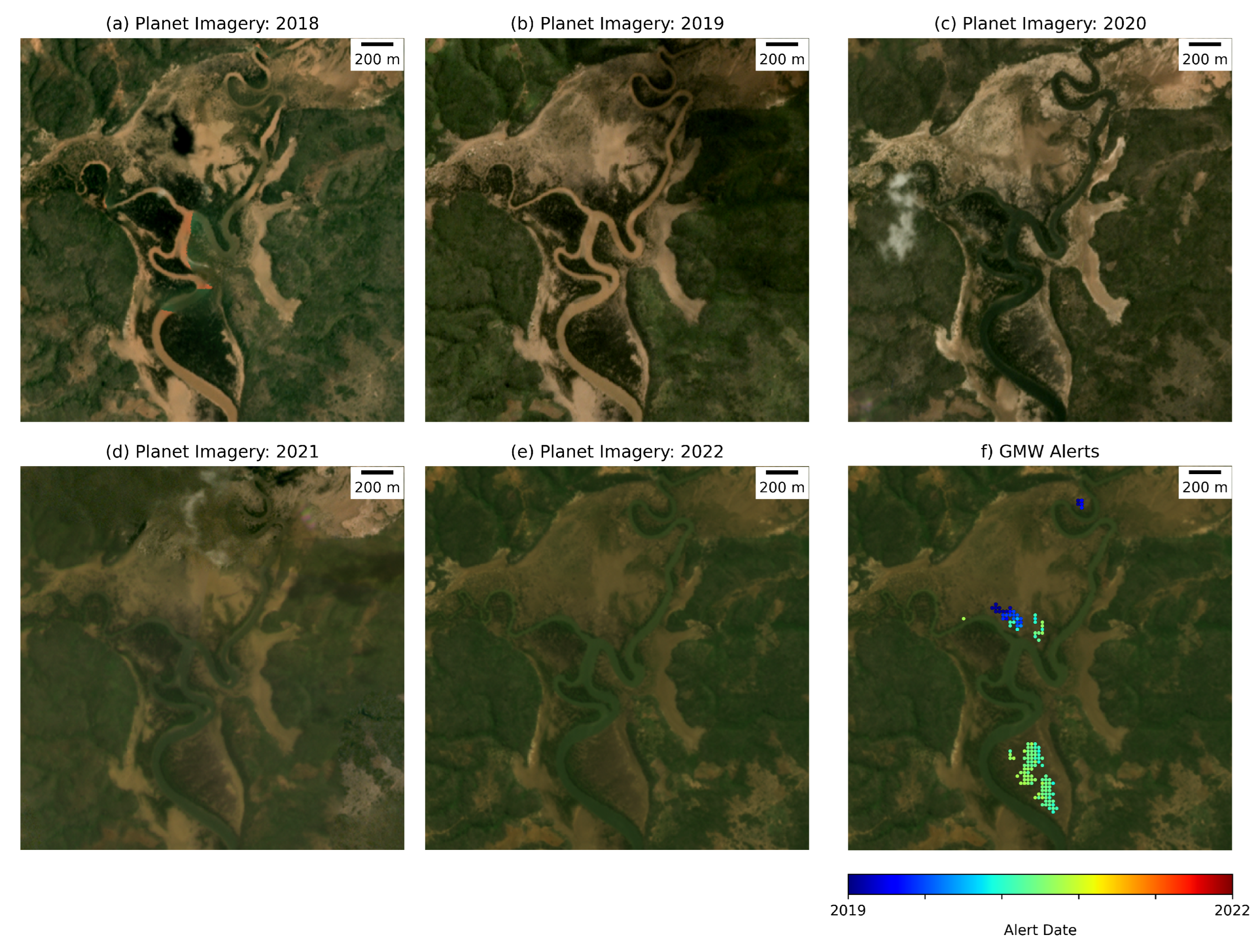
Remotesensing 15 02050 g012
Figure 13. A case study from Guinea-Bissau where a new dam was built, resulting in the mangroves behind the dam being removed for rice cultivation. (a) illustrates the Planet imagery before the dam was built, (be) the dam was built and mangroves lost over the period and (f) the GMW Mangrove Loss Alerts identified over the period. (Image courtesy: Planet Labs/NICFI, 2018).
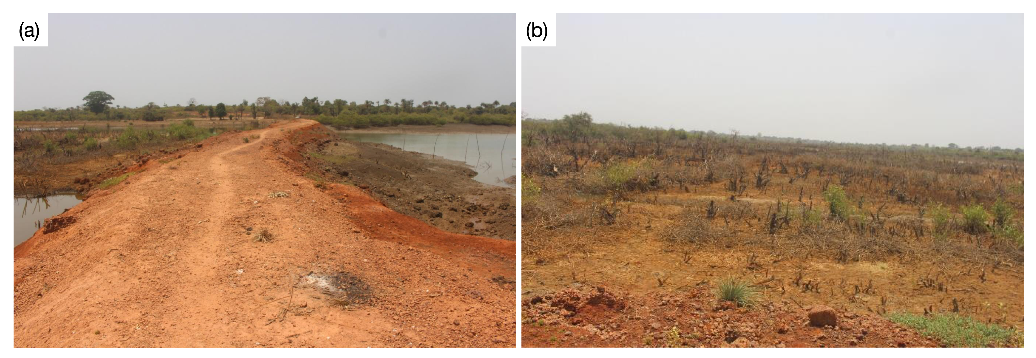
Remotesensing 15 02050 g013
Figure 14. Example field photos taken during the field visits to the area shown in Figure 13. (a) The dam was built to hold back the tidal waters allowing for rice cultivation. (b) An area behind the dam where mangroves have started to be removed to be converted into rice paddies. Credit: Wetlands International; Taken: 7 April 2021.
Remotesensing 15 02050 g014
Figure 15. A case study from Kenya where the alerts identified mangroves being lost due to charcoal production. (a) Illustrates the planet imagery before the mangrove loss, (be) mangroves lost over the period and (f) the GMW Mangrove Loss Alerts identified over the period. (Image courtesy: Planet Labs/NICFI).
Remotesensing 15 02050 g015
Figure 16. An area of mangroves which has been cut for charcoal production within the region shown in Figure 15. Rehabilitation activities have already started, with the mangrove seeding seen in this photo having been planted as part of that activity. Credit: Wetlands International; Taken: 1 December 2022.
Remotesensing 15 02050 g016
Table 1. Optimal thresholds identified for refining the mangrove extent for 2018. The index thresholds were applied to each scene to identify non-mangrove pixels. The count threshold was used to threshold the number of times a pixel has crossed the threshold combining the results from the individual scenes to create a single mask for each index. Acronym definitions: normalised difference vegetation index (NDVI), normalised difference water index (NDWI), mangrove vegetation index (MVI), Sentinel-1 vertical–horizontal (VH) polarisation.
IndexIndex ThresholdCount Threshold
NDVI<0.14
MVI<0.14
NDWI>−0.14
MNDWI>0.154
Min. Sentinel-1 VH<−19 [dB]-
Table 2. The upper part of the table provides the range of values tested during the sensitivity analysis to identify the optimal thresholds for the change analysis. The index threshold is the threshold to find a potential mangrove loss within an individual scene. The absolute difference threshold is the difference in the index between the current scene and the median pixel value for the month from the previous year. The score threshold is related to the number of times a change needs to have occurred for the mangrove loss alert to be confirmed. The bottom part of the table provides the resulting optimal thresholds identified through the sensitivity analysis. Acronym definitions: normalised difference vegetation index (NDVI), normalised difference water index (NDWI).
IndexIndex ThresholdAbs. Diff ThresholdScore Threshold
Sensitivity Analysis Test Values
NDVI0.05, 0.1, 0.15, 0.2, 0.25, 0.30.1, 0.15, 0.2, 0.25, 0.33, 5, 7, 9
NDWI−0.2, −0.15, −0.1, −0.05, 0.0, 0.050.1, 0.15, 0.2, 0.25, 0.33, 5, 7, 9
Optimal Thresholds
NDVI<0.250.155
NDWI>0.050.257
Table 3. Summarising the mangrove loss alerts results on a per-country basis. Including the number of mangrove loss alerts identified within each country, the GMW 2018 mangrove extent for the country, the spatial density of mangrove loss alerts for the country, provided as the number of hectares per mangrove loss alert (Num. ha per Alert; mangrove extent/number of alerts) and the number of mangrove loss alerts assigned to each change pressure for each country.
CountryNumber of Alerts2018 Mangrove Extent (Hectares)Num. ha per AlertAgricultureInfrastructureClearingErosionOther
Nigeria16,380845,3595203266399636115507
Guinea-Bissau13,012269,7782112,021183219922
Madagascar12,964277,2212100053312,431
Mozambique12,140309,56025010077011,360
Guinea10,722222,77421691736217596161068
Sierra Leone2659157,6295959992419082
Senegal1421127,03189000311390
Tanzania845111,542132818110511
Cameroon500196,877394014043353
Ghana48217,9503702400458
Kenya32754,32816607600251
Gambia24061,12225501710069
Angola21828,35813001470071
Benin1702941170060164
Liberia16118,69111606137018
Côte d’Ivoire65541183065000
Seychelles423829000042
Democratic Republic of the Congo1223,6591972000012
South Africa112648241110000
Djibouti1073874000010
Somalia8355444400008
Total72,3892,737,5533819,82642698349601833,927
Table 4. The accuracy assessment metrics using the 1 km hexagons to assess the accuracy of the mangrove loss alerts without reference to a mangrove baseline.
MetricMedian Estimate95th Confidence
Overall Accuracy92.1%89.0–95.7%
Cohen Kappa0.7890.704–0.865
Balanced Overall Accuracy88.0%83.1–93.3%
Macro F1-Score0.8940.851–0.937
Weighted Avg. F1-Score0.9200.887–0.956
Matthews Correlation Coefficient0.7920.709–0.876
Mangrove Loss Alerts
F1-Score0.8420.769–0.907
Precision/Users0.9000.813–0.967
Recall/Producers0.7940.696–0.892
Omission20.6%10.8–30.4%
Commission10.4%3.3–18.6%
No Mangrove Loss Class
F1-Score0.9480.926–0.970
Precision/Producers0.9300.896–0.963
Recall/Users0.9680.940–0.989
Omission3.2%1.1–6.0%
Commission7.0%3.7–10.4%
Table 5. The 1 km hexagon intersections between the GMW Mangrove Loss Alerts (this study), the JJ-Fast alerts [34] and GFW alerts [32,33]. This revealed a low correspondence between the three datasets, with only 14% of the GMW Mangrove Loss Alerts intersecting with the GFW and only 5% of the JJ-FAST and GMW alerts intersecting.
GMWGFWJJ-Fast
GMW2678397121
GFW14%166590
JJ-Fast5%7%1047
Table 6. Comparison of the accuracy of mapping mangrove loss between the GMW Mangrove Loss Alerts (this study), the JJ-FAST alerts [34] and GFW alerts [32,33].
MetricMedian Estimate95th Confidence
GMW Mangrove Loss Accuracy
F1-Score0.8420.769–0.907
Precision/Users0.9000.813–0.967
Recall/Producers0.7940.696–0.892
Omission20.6%10.8–30.4%
Commission10.4%3.3–18.6%
GFW Mangrove Loss Accuracy
F1-Score0.400.298–0.504
Precision/Producers0.5340.400–0.673
Recall/Users0.3210.229–0.425
Omission67.9%57.5–77.1%
Commission46.6%32.7–60.0%
JJ-Fast Mangrove Loss Accuracy
F1-Score0.1480.063–0.244
Precision/Producers0.2690.117–0.448
Recall/Users0.2000.042–0.177
Omission89.7%82.3–95.8%
Commission73.1%55.2–88.3%
Disclaimer/Publisher’s Note: The statements, opinions and data contained in all publications are solely those of the individual author(s) and contributor(s) and not of MDPI and/or the editor(s). MDPI and/or the editor(s) disclaim responsibility for any injury to people or property resulting from any ideas, methods, instructions or products referred to in the content.

