Article

Incorporation of Fused Remote Sensing Imagery to Enhance Soil Organic Carbon Spatial Prediction in an Agricultural Area in Yellow River Basin, China

1
School of Grassland Science, Beijing Forestry University, Beijing 100083, China
2
School of Forest Resources and Conservation—Geomatics Program, University of Florida, 301 Reed Lab, Gainesville, FL 32611, USA
3
Gulf Coast REC/School of Forest Resources and Conservation—Geomatics Program, University of Florida, 1200 N. Park Road, Plant City, FL 33563, USA
*
Author to whom correspondence should be addressed.
Remote Sens. 2023, 15(8), 2017; https://doi.org/10.3390/rs15082017
Submission received: 21 February 2023 / Revised: 4 April 2023 / Accepted: 6 April 2023 / Published: 11 April 2023
(This article belongs to the Section Remote Sensing in Agriculture and Vegetation)

Abstract

:
To overcome spatial, spectral and temporal constraints of different remote sensing products, data fusion is a good technique to improve the prediction capability of soil prediction models. However, few studies have analyzed the effects of image fusion on digital soil mapping (DSM) models. This research fused multispectral (MS) and panchromatic Landsat 8 (L8) bands, and MS Sentinel 2 (S2) and panchromatic L8 bands using the Brovey, Intensity–Hue–Saturation and Gram–Schmidt methods in an agricultural area in Yellow River Basin, China. To analyze the effects of image fusion on DSM models, various SOC prediction models derived from remote sensing image datasets were established by the random forest method. Soil salinity indices and spectral reflectance from all the remote sensing data had relatively strong negative correlations with SOC, and vegetation indices and water indices from all the remote sensing data had relatively strong positive correlations with SOC. Soil moisture and vegetation were the main controlling factors of the SOC spatial pattern in the study area. More spectral indices derived from pansharpened L8 and fused S2–L8 images by all three image fusion methods had stronger relationships with SOC compared with those from MS L8 and MS S2, respectively. All the SOC models established by pansharpened L8 and fused S2–L8 images had higher prediction accuracy than those established by MS L8 and MS S2, respectively. The fusion between S2 and L8 bands had stronger effects on enhancing the prediction accuracy of SOC models compared with the fusion between panchromatic and MS L8 bands. It is concluded that digital soil mapping and image fusion can be utilized to increase the prediction performance of SOC spatial prediction models.

1. Introduction

Soil is a crucial component of the ecological environment and closely related to food security and ecological functions including water retention, carbon sequestration, and climate change mitigation [1]. Assessing the spatial characteristics of soil nutrient contents in farmland can provide important information about soil fertility, sustainable soil management, food security and ecosystem health [2]. Digital soil mapping (DSM) techniques are important tools to show the spatial pattern of soil nutrients in wetland [3], forest [4], grassland [5] and farmland [6,7] areas. DSM can overcome the disadvantages of traditional soil mapping and has been widely utilized to quantify soil information with higher temporal–spatial resolution and model accuracy, and lower uncertainty [8]. Soil properties in agricultural ecosystems are highly dynamic and affected by human-induced activities including irrigation, fertilization, applications of pesticide and desertification [9]. They tend to show large spatial heterogeneity compared with other ecosystems. Unlike DSM research at the continental and national scales [2,10], the soil-landscape attributes of DSM including land use, parent material, climate conditions and topographic attributes at the county and township scales do not demonstrate strong spatial variations. As a result, remote sensing-based spectral indices can explain the spatial distribution of soil nutrients at the county and township scales [11]. Different remote sensing products, however, have their own characteristics and different spatial/spectral/temporal resolutions. The spectral indices derived from various remote sensing sensors have different capabilities to predict soil properties. For instance, L8 bands range from the visible to thermal infrared part of the electromagnetic spectrum. At the same time, L8 lacks a red-edge band and has medium spatial resolution (30 m). Although the spatial resolution of some remote sensing images including WorldView-2 and GeoEye-1 is 2 m, they do not have short-wave infrared and thermal infrared bands [12]. Data fusion of various remote sensing products with different spatial, temporal and spectral resolution is increasingly becoming a strong trend in remote sensing applications, which can provide important environmental factors capable of explaining the variations in soil properties at the local scale.
Among the advantages of data fusion is its outcome or response, which is more than the sum of the involved components [13,14]. Improved models and scientific understanding can be achieved through incorporating various datasets and methods that are coming from diverse disciplines [15,16]. Various studies already proved the importance of geospatial data fusion in different research fields. The authors of [17] fused Landsat 7 images (medium spatial and coarse temporal resolution) and MODIS images (coarse spatial and fine temporal resolution) to derive phenological information of an agricultural system in Germany. Data fusion of aerial photography and LiDAR can achieve automated volcano mapping with high accuracy [18]. The incorporation of multitemporal Synthetic Aperture Radar (SAR) and optical data can achieve higher prediction accuracy of crop types compared with standalone SAR or optical data [19].
The application of data fusion in DSM is still in its infancy, and the effect of data fusion on DSM is an active research topic. The incorporation of complementary satellite data including MODIS and S2 improved the clay content estimation of the topsoil layers in mainland France [20]. The integration of airborne hyperspectral and proximal sensing reduced the uncertainty of soil clay content prediction models [21]. Most research focused on the integration of laboratory spectral or proximal sensing in DSM, and the effect of image fusion on DSM is not clarified. The authors of [22] utilized the Brovey, Gram–Schmit (GS), and Intensity–Hue–Saturation (IHS) methods to fuse the multispectral bands and panchromatic band of L8, and concluded that DSM models of soil total nitrogen based on pansharpened (PAN) L8 had slightly higher prediction accuracy than MS L8-based models. Most of the studies utilizing image fusion just compared the DSM models based on MS and PAN images of the same imaging platform. Few studies have explored the effects of data fusion between different types of remote sensing images on DSM models.
Food security has long been a priority of developing countries due to the major challenges posed by the large population and limited agricultural land [23]. DSM techniques can explore site-specific soil fertility status of the farmland and help farmers identify soil quality problems over a large-scale agricultural area. Fusion and incorporation of different datasets, technologies and approaches can complement each other and improve spatial modeling of soil properties [24]. The aims of this research are to (1) analyze the relationships between soil organic carbon (SOC) and environmental factors including remote sensing predictors; (2) establish DSM models based on MS and fused remote sensing images, and compare prediction performances and predicted maps of DSM models; (3) explore the effects of the remote sensing image fusion on DSM in an agricultural fields in Yellow River Basin, China.

2. Materials and Methods

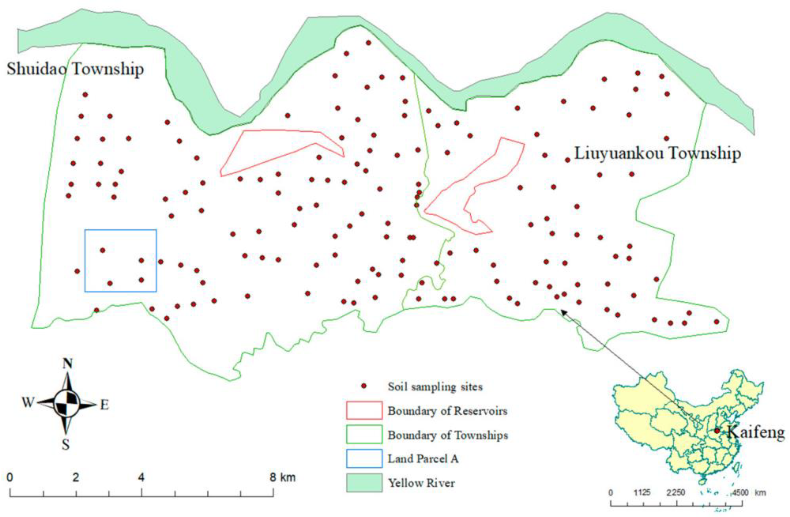
2.1. Study Area Description and Soil Sampling

Two townships called the Shuidao Township and Liuyuankou Township (114°11′–114°26′E, 34°49′–34°56′N) are located in the south of the Yellow River and the northern of Kaifeng City, Henan Province, China (Figure 1). Land Parcel A is in the southwest of the study area (Figure 1). The study area has a typical continental warm temperate zone monsoon climate, and there is a clear distinction between the four seasons. The average annual temperature is 14.52 °C, and average annual precipitation is 627.5 mm. The topography of the study area is dominated by plains, and its topographical relief is uniform. The soil texture in the study area is mainly clay loam and loam. The major crop systems are two double crop rotations including wheat (Triticum aestivum)-maize (Zea mays) and wheat (Triticum aestivum)-cotton (Gossypium hirsutum).
Four top soil samples (0–15 cm) were taken in a 5 m grid and mixed thoroughly into a composite sample. There were 155 composite soil samples acquired in June 2018 (Figure 1). All the soil samples were stored in plastic bags after plants and debris covering the soil surface were removed. Those soil samples were dried for 14 days and passed through a 2 mm sieve in the laboratory. The SOC content was determined using the Walkley–Black method [25].

2.2. Image Fusion

One cloud-free L8 remote sensing image (Acquisition date: 11 June 2018) was collected from the United States Geological Survey (USGS) website (https://earthexplorer.usgs.gov/, accessed on 12 March 2020). One cloud-free Sentinel-2 (Acquisition date: 12 June 2018) was collected from the European Space Agency website (https://scihub.copernicus.eu/, accessed on 12 March 2020). The co-registration of L8 and S2 data was performed using the ENVI software, and the co-registration error was smaller than a pixel.
The Brovey [26], Intensity–Hue–Saturation (IHS) [27] and Gram Schmidt (GS) [28,29] classical image fusion methods were applied to implement the image fusion in ArcGIS 10.4.1. The IHS method is a color-based fusion technique where RGB (red–green–blue) color space is converted to the IHS color space [30]. The Brovey method is an arithmetic-related technique, where each spectral band is first divided by the sum of the three chosen bands and then multiplied with the panchromatic band [31]. The GS method aims to produce a different set of bands by orthogonalizing bands of a remote sensing product [29]. Multispectral (MS) L8 bands (30 m) and panchromatic L8 band (15 m) were fused into Brovey, IHS and GS L8 images (15 m) (Figure S1). After transforming the spatial resolution of all the S2 bands to 20 m by Resample Tool (nearest neighborhood method) in ArcGIS 10.4.1, MS S2 bands (20 m) and panchromatic L8 band (15 m) were fused into Brovey, IHS and GS fused S2–L8 images (15 m) (Figure S3).

2.3. Environmental Data Extraction

Table S1 listed all the environmental variables in this research. Spectral reflectances of different bands, band ratios between different bands, red band-based vegetation indices including the Normalized Difference Vegetation Index (NDVI), red-edge-band-based vegetation indices including the Normalized Difference Red-edge Index (NDVIr), bare soil indices including the Normalized Difference Soil Index (NDSI), water indices including the Normalized Difference Water Index (NDWI), temperature indices including the at-satellite brightness temperature for thermal bands (T1, T2), and salinity indices including Salinity Index 1 (SI1) were acquired from MS L8 image, PAN L8 images, MS S2 image, and fused S2–L8 images. Topographic attributes were extracted from the GTOPO30 digital elevation model (DEM) with 30 m resolution acquired from the USGS website (https://earthexplorer.usgs.gov/, accessed on 20 March 2020). Principal component analysis (PCA) is the algorithm that can identify the optimum linear combination of the original image bands and account for most of the variation in pixel values [32]. PCA of the ArcGIS tool was employed to derive PC scores (P1, P2 and P3) for bands of remote sensing imagery. In addition, geographic attributes and crop types were also chosen as environmental factors in this research. All the environmental data in Table S1 were transformed to the Universal Transverse Mercator map projection (Zone: 50 N; Datum: WGS 1984).

2.4. Model Calibration and Validation

2.4.1. Model Calibration

Soil samples were separated into a calibration dataset (70% of the total samples: 109 samples) and a validation dataset (30% of total samples: 46 samples). The calibration datasets were utilized to establish spatial prediction models of SOC, while the validation datasets were utilized for validation. This research established 8 models including SOC prediction models based on MS L8 (LT model) (spatial resolution: 30 m), Brovey L8 (LTb model) (15 m), IHS L8 (LTi model) (15 m), GS L8 (LTg model) (15 m), MS S2 (ST model) (20 m), Brovey fused S2–L8 (STb model) (15 m), IHS fused S2–L8 (STi model) (15 m), and GS fused S2–L8 (STg model) (15 m). By comparing the model performance and DSM maps of those 8 models, this research aims to reveal the effects of image fusion on DSM.
Environmental factors which are relevant to the SOC were identified using the Boruta algorithm [33]. The Boruta algorithm is an ensemble method in which classification is performed by voting of multiple unbiased weak classifier decision trees, and it can identify linear and nonlinear relationships between soil properties and environmental factors [33,34]. Optimal variables identified by the Boruta algorithm (Figure 2 and Figure 3) were utilized as predictors to develop SOC prediction models based on random forest (RF) method.
RF is a tree-based prediction model developed by [35]. RF method can accommodate different types of input data, and deal with non-linearity between the environmental factors and target soil properties including SOC, and the interaction between the environmental factors. Multiple trees were developed by using a modified bootstrap aggregation (bagging) algorithm. Model predictions are then estimated as weighted averages across all trees. The optimization of the number of trees (ntree), and the number of variables as a predictor at each tree (mtry) were conducted by using different combinations of ntree and mtry. The ntree was set between 100 and 900 at intervals of 200, and the mtry was set between 1 and 15 at 1 interval. Model establishment and soil mapping were conducted using R packages including the “Boruta”, “randomForest”, “raster”, “caret” and “rgdal” in the R statistical software (version: 2.1.1) (R Development Core Team, R Foundation for Statistical Computing, Vienna, Austria, 2013).

2.4.2. Model Validation

Model validation was used to analyze the prediction performance of different SOC models. The results were assessed using the coefficient of determination (R2), root mean square error (RMSE), and ratio of performance to deviation (RPD) obtained from the observed and predicted values of SOC [36].

3. Results

3.1. Statistical Summary of SOC Concentration

The SOC content of the topsoil (0–15 cm) ranged from 2.03 g/kg to 26.28 g/kg. The mean values of the total, calibration and validation datasets were 11.15, 11.10 and 11.27 g/kg, with standard deviations (SDs) of 5.83, 5.75 and 6.10 g/kg. The descriptive statistical summaries of the whole, calibration and validation dataset were similar as shown in Table 1, showing calibration and validation datasets were representative for the model calibration and validation, respectively.

3.2. Relationships between SOC and Remote Sensing Predictors

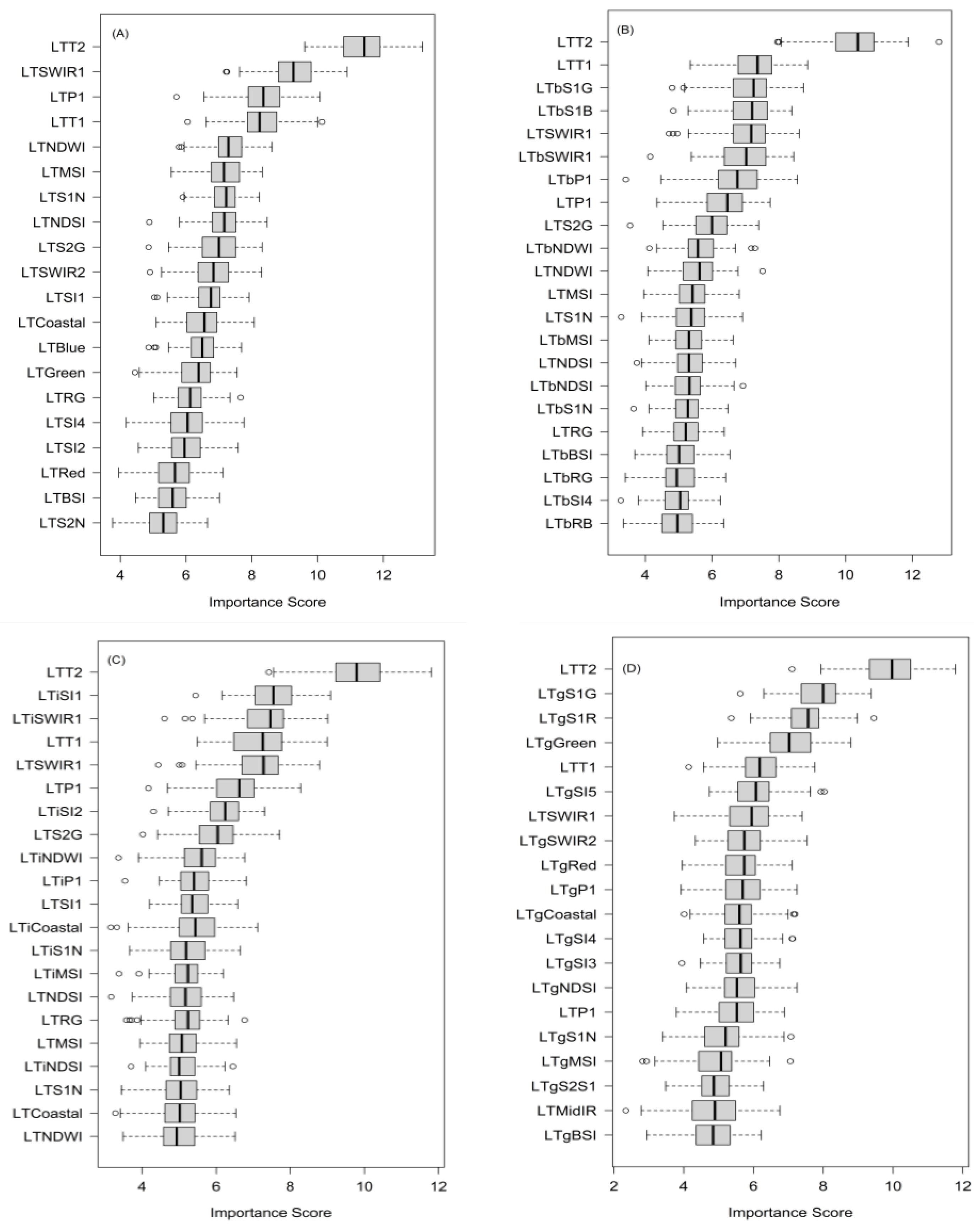
3.2.1. Relationships between SOC and L8-Based Spectral Indices

Multiple L8-based spectral indices showed relatively strong positive or negative linear relationships with SOC (Table 2). Band reflectances including short-wave infrared reflectance (LTSWIR1, LTSWIR2), red reflectance (LTRed) and blue reflectance (LTBlue); band ratios of short-wave infrared (SWIR) bands to near infrared (NIR) band (LTS2N, LTS1N); at-satellite brightness temperatures for L8 band 11 (LTT2); and bare soil indices including the Normalized Difference Soil Index (LTNDSI), and soil salinity indices including Salinity Index 1 (LTSI1) had relatively strong negative correlations with SOC. In contrast, vegetation indices including the Normalized Difference Vegetation Index (LTNDVI) and Simple Ratio (LTSR), and water indices including the Normalized Difference Water Index (LTNDWI) had relatively strong positive correlations with SOC. After incorporating PAN L8 spectral indices, multiple PAN L8-based spectral indices had stronger linear relationships with SOC compared with the MS L8-based spectral indices (Table 2). The ratio of short-wave infrared band 1 to green band (S1G) and the NDWI extracted from GS L8 (LTg) had stronger linear relationships with SOC than all the MS L8-based spectral indices.
The L8-based spectral indices selected by the Boruta algorithm were shown in Figure 2. Those spectral indices were utilized as the predictors in the LT model (Figure 2A), the LTb model (Figure 2B), the LTi model (Figure 2C), and the LTg model (Figure 2D). The at-satellite brightness temperature for L8 band 11 (LTT2) had highest importance score among all the L8 spectral indices. Principal component band 1 for L8 bands (LTP1), short-wave infrared band reflectances (LTSWIR1 and LTSWIR2) and water indices (LTNDWI and LTMSI) also had relatively high importance scores among all the MS L8 spectral indices (Figure 2A). Some Brovey L8 spectral indices including the band ratios of SWIR band 1 to green band (LTbS1G), SWIR band 1 to blue band (LTbS1B), SWIR band 1 spectral reflectance (LTbSWIR1) and principal component score 1 (LTbP1) were also selected as optimal variables with SOC (Figure 2B). Multiple IHS L8 spectral indices including soil salinity indices (LTiSI1 and LTiSI2), LTiSWIR1, and LTiNDWI had high importance scores (Figure 2C). The ratio of short-wave infrared band 1 to green band (LTgS1G), and the ratio of short-wave infrared band 1 to red band (LTgS1R) from GS L8 had relatively higher importance scores than other spectral indices (Figure 2D).

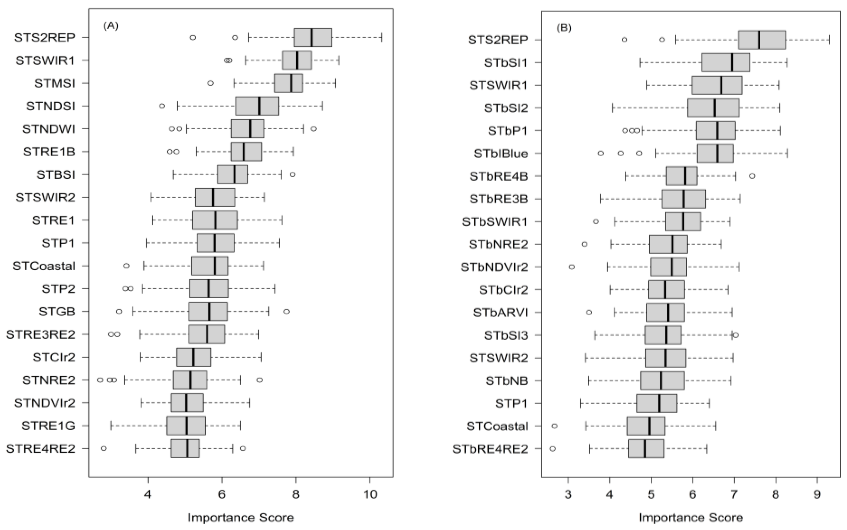
3.2.2. Relationships between SOC and S2-Based Spectral Indices

The spectral behavior between S2-based spectral indices and SOC was similar to that between L8-based spectral indices and SOC (Table 3). Multiple spectral reflectances including SWIR reflectances (STSWIR1, STSWIR2) and red edge (RE) band 1 reflectance (STRE1), band ratios including STRE1B; and bare soil indices including the STNDSI and the STBSI had relatively strong negative correlations with SOC. The Red-Edge (RE) band-related vegetation indices including the STNDVIr1, and STCIr1 had relatively strong positive correlations with SOC. There is no red band-based vegetation indices such as the NDVI and ARVI from S2 were listed in Table 3. Multiple spectral indices extracted from PAN fused S2–L8 images had stronger correlations with SOC than those from MS S2 (Table 3). Soil Salinity Index 2 from IHS fused S2–L8 image (STiSI2) had the strongest correlations with SOC among all the environmental factors. The results from Table 3 suggested the spectral indices from fused S2–L8 images had significantly stronger correlations with SOC compared with spectral indices from MS S2 image.
The S2-based spectral indices selected by the Boruta algorithm were shown in Figure 3. Those spectral indices were utilized as the predictors in the ST model (Figure 3A), the STb model (Figure 3B), the STi model (Figure 3C), and STg the model (Figure 3D). S2 Red-Edge Position (STS2REP) from MS S2 had the highest importance scores. Multiple RE-related spectral indices from Brovey fused S2–L8 image including band ratio of RE band 4 to blue (STbRE4B), NIR band to RE band 2 (STbNRE2) and the Normalized Difference Red-edge Index (STbNDVIr2) had high importance scores (Figure 3B). Soil salinity indices (STiSI2, STiSI1), band reflectances (STiBlue, STiGreen, STiSWIR1), band ratio of RE bands to other bands (STiRE3B, STiRE4B, STiRE4G), RE band-based vegetation indices (STiCIr2 and STiTCARI2) from IHS fused S2–L8 image were identified as optimal variables (Figure 3C). Band ratio between near infrared band to RE band 2 (STgNRE2) and SWIR1 (STgSWIR1) from GS fused S2–L8 image had relatively high importance scores (Figure 3D). Overall, much more fused S2–L8 spectral indices had higher correlations and importance scores than MS S2 spectral indices.

3.3. Spatial Prediction of SOC

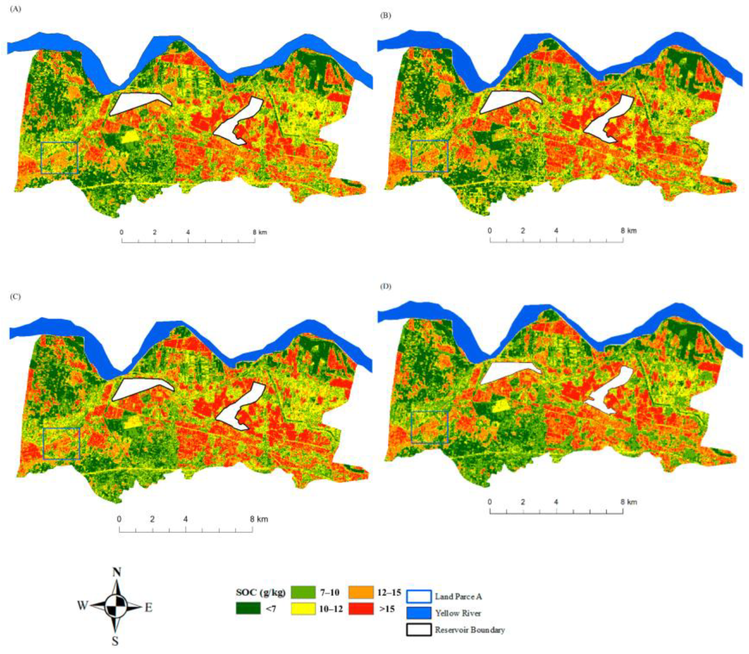
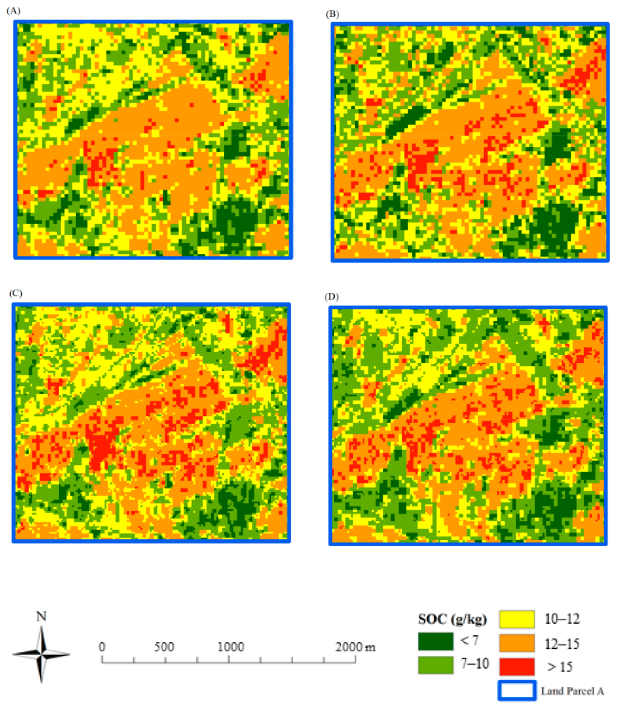
3.3.1. Spatial Prediction of SOC Based on MS and PAN L8 Imagery

Figure 4 showed the spatial variation of SOC based on four models (LT, LTb, LTi and LTg) in the study area. The overall SOC concentration in the convex area adjacent to the Yellow River (Figure 4) was at a low level in general. The farmlands which are adjacent to the two reservoirs (Figure 4) showed relatively high SOC concentration. In addition, overall SOC concentration in the Shuidao Township (west of the study area) was relatively lower than that in the Liuyuankou Township (east of the study area). The linear pattern of low SOC in village roads and delicate SOC variation of different land parcels were clearly depicted in the maps. Figure 5 showed the difference between maps produced by four models more clearly. Although all maps in Figure 5 showed alike spatial distribution of SOC, Figure 5B–D produced by PAN L8 spectral indices demonstrated more distinct spatial variation in Land Parcel A (Figure S2) compared with Figure 5A based on MS L8 spectral indices.

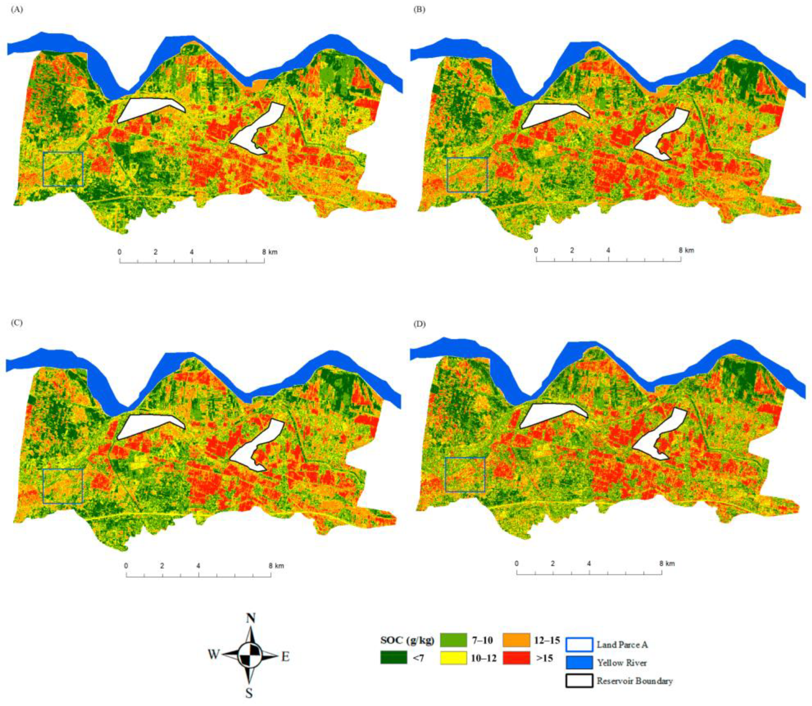
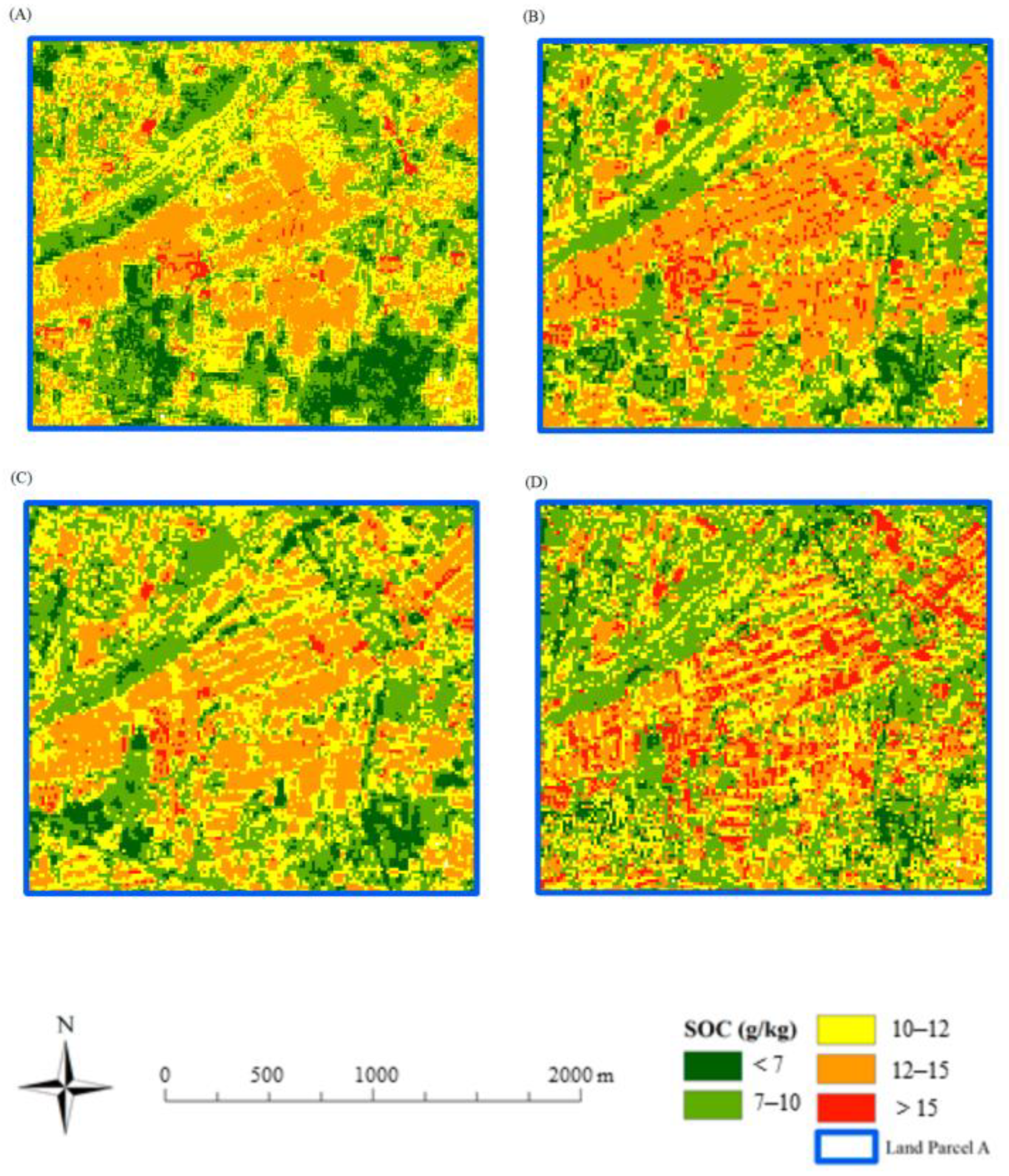
3.3.2. Spatial Prediction of SOC Based on MS S2 and Fused S2–L8 Imagery

Although model predictors used in the analysis were different, the spatial pattern of SOC based on MS S2 and fused S2–L8 images (Figure 6) was similar to that based on L8 images (Figure 4). The SOC in the four maps in Figure 6 shows mosaic spatial pattern with high heterogeneity from visual analysis. The dissimilarity was more obvious from visual analysis in Land Parcel A (Figure 7). Although all the four maps showed higher SOC concentration in the farmlands located in the middle of the Land Parcel A (Figure S4), the SOC map based on MS S2 spectral indices (Figure 7A) barely revealed the internal variation of SOC in those farmlands. The other three maps, especially Figure 7D, displayed the rectangular spatial pattern of SOC in the farmlands located in the middle of the Land Parcel A.

3.4. Comparison of Different SOC Models

All the SOC models based on fused spectral indices had higher prediction accuracy and lower prediction uncertainty than those based MS spectral indices (Table 4). However, the model performance difference between fused S2–L8 and MS S2 models is more evident than that between PAN L8 and MS L8 models. For example, the R2 (0.67) and RPD (1.69) of LTg were 31% and 18% higher than the R2 (0.51) and RPD (1.43) of the LT model, respectively, and the R2 (0.57) and RPD (1.53) of STg were 58% and 23% higher than the R2 (0.36) and RPD (1.24) of the ST model, respectively.

4. Discussion

4.1. Controlling Factors of SOC

Topographic attributes had relatively weak correlations and low importance scores with SOC, suggesting they were not among the main factors that control the SOC spatial distribution. It is noticeable that topographic attributes including elevation and slope were relatively homogeneous in this agricultural area of North China Plain. Most environmental factors selected as optimal variables were remote sensing predictors (Figure 2 and Figure 3). This suggests the importance of remote sensing predictors in predicting soil properties in plain agricultural area. Multiple research already indicated that spectral reflectance decreases with the increase in soil water content [37,38]. The negative correlations between spectral reflectances and SOC from L8 and S2 imply that higher soil moisture (lower spectral reflectance) contribute to the accumulation of SOC. The positive correlations between the NDWI and SOC suggests the potential positive feedback between soil moisture and SOC. The positive feedback between soil moisture and SOC confirmed the contribution of soil moisture on soil organic carbon sequestration, which is noticed in other agricultural areas in Canada [39] and Brazil [40].
The positive association between vegetation indices and SOC also imply that the more vegetated farmlands are more likely to have more SOC compared with less vegetated farmlands. Although large areas of soils were covered with plants and crops in remote sensing images, vegetation indices become good predictors for SOC as SOC is closely related to aboveground biomass and net primary productivity [41,42]. S2 Red-Edge Position (STS2REP) is ranked as the most important spectral index among all the S2 spectral indices. STS2REP was tested to have very strong relationship with leaf chlorophyll concentration, and it is a surrogate measure of vegetation chlorophyll content [43]. The inclusion of red-edge-band-based spectral indices as model predictors can mitigate the saturation effect at higher canopy chlorophyll content compared with red band-based spectral indices, and better reflect the health and function of aboveground vegetation and SOC. Most S2 spectral indices identified as optimal variables were RE band-based spectral indices (Figure 3), suggesting that four RE bands of S2 images have stronger capability to explain the SOC spatial variation compared with other bands. It is possible that RE band-based spectral indices had stronger capability in predicting the vegetation compared with NIR band-based spectral indices, as they are more sensitive to chlorophyll content and can overcome the saturation problem [44]. Vegetation is an important factors that can reflect the SOC distribution due to the significant influence of the SOC on the growth status and quality of crops in agricultural land [45,46]. The at-satellite brightness temperature of L8 image had the highest importance scores, indicating the strong potential of long wavelength (thermal) bands from L8 in predicting SOC.
The large farmland areas at the north of the study area, which are also adjacent to Yellow River, had relatively low SOC concentration. The long-term washing and flooding caused by the Yellow River could have led to soil erosion and SOC decrease in farmland near the river. The SOC concentration in the farmlands adjacent to the two reservoirs in the study area was at high levels, which also suggest the effect of soil moisture on SOC. In general, SOC is mainly affected by soil moisture and vegetation in the study area.

4.2. Effect of Remote Sensing Fusion on DSM

Various research have already proven that it is not possible to find the best remote sensing product for DSM as different remote sensing products have their own advantages and disadvantages in terms of spatial/spectral/temporal resolutions, purchase expenses and data quality [47,48]. As a result, data fusion is a good method that can take advantage of various remote sensing products and contribute to the model performance of DSM. Most of the research did not perform the image fusion, and they just analyzed the combination of different remote sensing sensor on digital soil mapping [49,50]. This research analyzed the effects of data fusion between MS and PAN bands of a single remote sensing product (L8) and two different remote sensing products (S2 and L8) on DSM. The spectral behavior of the fused images was similar to the original MS images. For example, vegetation indices and water indices from both the MS and fused images showed positive relationships with SOC (Table 2 and Table 3). More PAN L8 and fused S2–L8 spectral indices were selected as optimal variables than MS L8 and MS S2 spectral indices, respectively. This suggests that the fused spectral indices can explain the variation of SOC spatial distribution more precisely compared with MS spectral indices. This result confirms the advantages of image fusion, which does not only integrates the spectral information from the source images, but also preserves the spectral information of the source images [51].
Table 4 indicates that the fusion of PAN L8 spectral indices slightly enhanced the prediction performance of MS L8-based SOC model. It is possible that spectral information of MS and PAN bands from L8 are similar, and the fusion between MS and panchromatic bands from L8 could not overcome the limitation of L8 products. In comparison, the integration of fused S2–L8 spectral indices remarkably enhanced the prediction performance of the MS S2-based SOC model. The results suggest the potential advantages of fusion between different images on enhancing the predictive performance of DSM over fusion between MS and panchromatic bands from a single image. The data fusion between MS S2 bands and the L8 panchromatic band overcame the limitations from a single remote sensing sensor. Hence, both sensors’ spatial and spectral information can be utilized or partially utilized by the data fusion techniques. Although the three SOC maps derived from PAN L8 (Figure 5B–D) and fused S2–L8 (Figure 7B–D) had the same spatial resolution (15 m), Figure 7B–D showed higher spatial heterogeneity and more evident patch distribution in different farmlands compared with Figure 5B–D. In summary, the fusion between bands from different remote sensing products has stronger effects on enhancing SOC prediction accuracy compared with the fusion between bands from a single remote sensing product.

4.3. Prospect of Soil Spatial Prediction Models in Developing Countries

The application of DSM can pinpoint the controlling factors of the spatial pattern of soil properties, help farmers and policy makers understand the spatial characteristics of soil nutrient concentration, identify the farmland with low soil fertility, and implement soil improvement measures and increase soil quality and crop production [52]. Vegetation cover, soil moisture, surface roughness and management practices can also affect the soil prediction model performances. Developing soil prediction models with high temporal and spatial resolution and predictive capability has high potential to promote sustainable farm management in developing countries such as India and China. Soil organic carbon stocks of Western Ghats were predicted by Quantile Regression Forest algorithm by incorporating derivatives of the digital elevation model, L8 and MODIS images [53]. Multiple geostatistical and data mining methods were utilized to predict major soil nutrients in Northwestern China, and explored the effect mechanism between the spatial pattern of soil nutrients and farmland management practice [54]. As L8 and S2 are free to download, and have fair spatial, spectral and temporal resolutions, they are widely used in DSM. The results from this research also proved that the application of image fusion can not only enhance the prediction accuracy of DSM, but also increase the spatial resolution of soil maps. In the future, models of other soil properties can be developed using digital soil mapping and image fusion techniques in vast agricultural areas with different topographic and climate conditions.

5. Conclusions

MS and PAN L8 spectral indices such as spectral reflectances, soil salinity indices, the at-satellite brightness temperature, vegetation indices including the NDVI, TVI, and water indices including the NDWI showed relatively strong correlations and high importance scores with SOC. Spectral reflectances, vegetation indices derived from the red edge band including the NDVIr, CIr1 and S2REP from MS S2 and fused S2–L8 images had strong correlations and high importance scores with SOC. More PAN L8 spectral indices were chosen as optimal variables with SOC than MS L8 spectral indices. More fused S2–L8 spectral indices were chosen as optimal variables with SOC than MS S2 spectral indices. In general, SOC spatial distribution is mainly affected by soil moisture and vegetation in the study area. All the SOC models based on fused remote sensing images had higher prediction performances compared with those based on MS remote sensing images. The data fusion between bands from L8 and S2 has stronger effects on enhancing SOC prediction accuracy compared with the fusion between bands from L8. Image fusion techniques can be utilized in DSM research to increase model performance of soil prediction model, and this research provide a new idea for future DSM research.

Supplementary Materials

The following supporting information can be downloaded at: https://www.mdpi.com/article/10.3390/rs15082017/s1, Figure S1. Remote sensing images of (A) MS Landsat 8, (B) Brovey PAN Landsat 8, (C) IHS PAN Landsat 8 and (D) GS PAN Landsat 8 images in the study area; Figure S2. Remote sensing images of (A) MS Landsat 8, (B) Brovey PAN Landsat 8, (C) IHS PAN Landsat 8 and (D) GS PAN Landsat 8 images in the Land Parcel A; Figure S3. Remote sensing images of (A) MS Sentinel 2, (B) Brovey fused Sentinel 2-Landsat 8, (C) IHS fused Sentinel 2-Landsat 8 and (D) GS fused Sentinel 2-Landsat 8 in the study area; Figure S4. Remote sensing images of (A) MS Sentinel 2, (B) Brovey fused Sentinel 2-Landsat 8, (C) IHS fused Sentinel 2-Landsat 8 and (D) GS fused Sentinel 2-Landsat 8 in Land Parcel A; Table S1. Assembled environmental variables in the study area. References [43,55,56,57,58,59,60,61,62,63,64,65] are cited in the Supplementary Materials.

Author Contributions

Y.X. collected and processed the data, performed analysis, and wrote this paper; A.A.-E. proposed the main idea and made suggestions on the experiments; Y.T. helped to write and edit this article; T.F. and Q.W. analyzed the results and contributed to the validation. All authors have read and agreed to the published version of the manuscript.

Funding

This research was funded by the Fundamental Research Funds for the Central Universities (grant number BLX202165) and National Natural Science Foundation of China (No. 42001107).

Data Availability Statement

Not applicable.

Conflicts of Interest

The authors declare no conflict of interest.

References

  1. Payen, F.T.; Sykes, A.; Aitkenhead, M.; Alexander, P.; Moran, D.; MacLeod, M. Soil Organic Carbon Sequestration Rates in Vineyard Agroecosystems under Different Soil Management Practices: A Meta-Analysis. J. Clean. Prod. 2021, 290, 125736. [Google Scholar] [CrossRef]
  2. Liang, Z.; Chen, S.; Yang, Y.; Zhou, Y.; Shi, Z. High-Resolution Three-Dimensional Mapping of Soil Organic Carbon in China: Effects of SoilGrids Products on National Modeling. Sci. Total Environ. 2019, 685, 480–489. [Google Scholar] [CrossRef] [PubMed]
  3. Goldman, M.A.; Needelman, B.A.; Rabenhorst, M.C.; Lang, M.W.; McCarty, G.W.; King, P. Digital Soil Mapping in a Low-Relief Landscape to Support Wetland Restoration Decisions. Geoderma 2020, 373, 114420. [Google Scholar] [CrossRef]
  4. Mansuy, N.; Valeria, O.; Laamrani, A.; Fenton, N.; Guindon, L.; Bergeron, Y.; Beaudoin, A.; Légaré, S. Digital Mapping of Paludification in Soils under Black Spruce Forests of Eastern Canada. Geoderma Reg. 2018, 15, e00194. [Google Scholar] [CrossRef]
  5. Wang, S.; Fan, J.; Zhong, H.; Li, Y.; Zhu, H.; Qiao, Y.; Zhang, H. A Multi-Factor Weighted Regression Approach for Estimating the Spatial Distribution of Soil Organic Carbon in Grasslands. Catena 2019, 174, 248–258. [Google Scholar] [CrossRef]
  6. Bogunovic, I.; Pereira, P.; Brevik, E.C. Spatial Distribution of Soil Chemical Properties in an Organic Farm in Croatia. Sci. Total Environ. 2017, 584–585, 535–545. [Google Scholar] [CrossRef] [PubMed] [Green Version]
  7. Xu, Y.; Smith, S.E.; Grunwald, S.; Abd-Elrahman, A.; Wani, S.P.; Nair, V.D. Estimating Soil Total Nitrogen in Smallholder Farm Settings Using Remote Sensing Spectral Indices and Regression Kriging. Catena 2018, 163, 111–122. [Google Scholar] [CrossRef] [Green Version]
  8. Chen, S.; Arrouays, D.; Mulder, V.L.; Poggio, L.; Minasny, B.; Roudier, P.; Libohova, Z.; Lagacherie, P.; Shi, Z.; Hannam, J.; et al. Digital Mapping of GlobalSoilMap Soil Properties at a Broad Scale: A Review. Geoderma 2022, 409, 115567. [Google Scholar] [CrossRef]
  9. Van Shi, Z.; van Groenigen, K.J.; Osenberg, C.W.; Andresen, L.C.; Dukes, J.S.; Hovenden, M.J.; Luo, Y.; Michelsen, A.; Pendall, E. Predicting Soil Carbon Loss with Warming. Nature 2018, 554, E4–E5. [Google Scholar] [CrossRef]
  10. Padarian, J.; Minasny, B.; McBratney, A.B. Chile and the Chilean Soil Grid: A Contribution to GlobalSoilMap. Geoderma Reg. 2017, 9, 17–28. [Google Scholar] [CrossRef]
  11. Xu, Y.; Smith, S.E.; Grunwald, S.; Abd-Elrahman, A.; Wani, S.P. Incorporation of Satellite Remote Sensing Pan-Sharpened Imagery into Digital Soil Prediction and Mapping Models to Characterize Soil Property Variability in Small Agricultural Fields. ISPRS J. Photogramm. Remote Sens. 2017, 123, 1–19. [Google Scholar] [CrossRef] [Green Version]
  12. Wieland, M.; Martinis, S.; Kiefl, R.; Gstaiger, V. Semantic Segmentation of Water Bodies in Very High-Resolution Satellite and Aerial Images. Remote Sens. Environ. 2023, 287, 113452. [Google Scholar] [CrossRef]
  13. Abowarda, A.S.; Bai, L.; Zhang, C.; Long, D.; Li, X.; Huang, Q.; Sun, Z. Generating Surface Soil Moisture at 30 m Spatial Resolution Using Both Data Fusion and Machine Learning toward Better Water Resources Management at the Field Scale. Remote Sens. Environ. 2021, 255, 112301. [Google Scholar] [CrossRef]
  14. Ghassemian, H. A Review of Remote Sensing Image Fusion Methods. Inf. Fusion 2016, 32, 75–89. [Google Scholar] [CrossRef]
  15. Fletcher, R.J., Jr.; Fletcher, T.J.; Robertson, E.P.; Zuckerberg, B.; McCleery, R.A.; Dorazio, R.M. A Practical Guide for Combining Data to Model Species Distributions. Ecology 2019, 100, e02710. [Google Scholar] [CrossRef]
  16. Peters, D.P.C. Accessible Ecology: Synthesis of the Long, Deep, and Broad. Trends Ecol. Evol. 2010, 25, 592–601. [Google Scholar] [CrossRef]
  17. Möller, M.; Gerstmann, H.; Gao, F.; Dahms, T.C.; Förster, M. Coupling of Phenological Information and Simulated Vegetation Index Time Series: Limitations and Potentials for the Assessment and Monitoring of Soil Erosion Risk. Catena 2017, 150, 192–205. [Google Scholar] [CrossRef]
  18. Kereszturi, G.; Schaefer, L.N.; Schleiffarth, W.K.; Procter, J.; Pullanagari, R.R.; Mead, S.; Kennedy, B. Integrating Airborne Hyperspectral Imagery and LiDAR for Volcano Mapping and Monitoring through Image Classification. Int. J. Appl. Earth Obs. Geoinformation 2018, 73, 323–339. [Google Scholar] [CrossRef]
  19. Adrian, J.; Sagan, V.; Maimaitijiang, M. Sentinel SAR-Optical Fusion for Crop Type Mapping Using Deep Learning and Google Earth Engine. ISPRS J. Photogramm. Remote Sens. 2021, 175, 215–235. [Google Scholar] [CrossRef]
  20. Loiseau, T.; Chen, S.; Mulder, V.L.; Román Dobarco, M.; Richer-de-Forges, A.C.; Lehmann, S.; Bourennane, H.; Saby, N.P.A.; Martin, M.P.; Vaudour, E.; et al. Satellite Data Integration for Soil Clay Content Modelling at a National Scale. Int. J. Appl. Earth Obs. Geoinf. 2019, 82, 101905. [Google Scholar] [CrossRef]
  21. Ciampalini, A.; André, F.; Garfagnoli, F.; Grandjean, G.; Lambot, S.; Chiarantini, L.; Moretti, S. Improved Estimation of Soil Clay Content by the Fusion of Remote Hyperspectral and Proximal Geophysical Sensing. J. Appl. Geophys. 2015, 116, 135–145. [Google Scholar] [CrossRef]
  22. Xu, Y.; Smith, S.E.; Grunwald, S.; Abd-Elrahman, A.; Wani, S.P. Effects of Image Pansharpening on Soil Total Nitrogen Prediction Models in South India. Geoderma 2018, 320, 52–66. [Google Scholar] [CrossRef]
  23. van Dijk, M.; Morley, T.; Rau, M.L.; Saghai, Y. A Meta-Analysis of Projected Global Food Demand and Population at Risk of Hunger for the Period 2010–2050. Nat. Food 2021, 2, 494–501. [Google Scholar] [CrossRef]
  24. Di Curzio, D.; Castrignanò, A.; Fountas, S.; Romić, M.; Viscarra Rossel, R.A. Multi-Source Data Fusion of Big Spatial-Temporal Data in Soil, Geo-Engineering and Environmental Studies. Sci. Total Environ. 2021, 788, 147842. [Google Scholar] [CrossRef]
  25. Walkley, A.; Black, I.A. An examination of the degtjareff method for determining soil organic matter, and a proposed modification of the chromic acid titration method. Soil Sci. 1934, 37, 29. [Google Scholar] [CrossRef]
  26. Ehlers, M.; Klonus, S.; Åstrand, P.J.; Rosso, P. Multi-Sensor Image Fusion for Pansharpening in Remote Sensing. Int. J. Image Data Fusion 2010, 1, 25–45. [Google Scholar] [CrossRef]
  27. Daneshvar, S.; Ghassemian, H. MRI and PET Image Fusion by Combining IHS and Retina-Inspired Models. Inf. Fusion 2010, 11, 114–123. [Google Scholar] [CrossRef]
  28. Dadrass Javan, F.; Samadzadegan, F.; Mehravar, S.; Toosi, A.; Khatami, R.; Stein, A. A Review of Image Fusion Techniques for Pan-Sharpening of High-Resolution Satellite Imagery. ISPRS J. Photogramm. Remote Sens. 2021, 171, 101–117. [Google Scholar] [CrossRef]
  29. Laben, C.A.; Brower, B.V. Process for Enhancing the Spatial Resolution of Multispectral Imagery Using Pan-Sharpening. U.S. Patent No. 6,011,875, 4 January 2000. [Google Scholar]
  30. Thomas, C.; Ranchin, T.; Wald, L.; Chanussot, J. Synthesis of Multispectral Images to High Spatial Resolution: A Critical Review of Fusion Methods Based on Remote Sensing Physics. IEEE Trans. Geosci. Remote Sens. 2008, 46, 1301–1312. [Google Scholar] [CrossRef] [Green Version]
  31. Du, Q.; Younan, N.H.; King, R.; Shah, V.P. On the Performance Evaluation of Pan-Sharpening Techniques. IEEE Geosci. Remote Sens. Lett. 2007, 4, 518–522. [Google Scholar] [CrossRef]
  32. Neeti, N.; Ronald Eastman, J. Novel Approaches in Extended Principal Component Analysis to Compare Spatio-Temporal Patterns among Multiple Image Time Series. Remote Sens. Environ. 2014, 148, 84–96. [Google Scholar] [CrossRef]
  33. Rudnicki, W.; Kursa, M. Feature Selection with the Boruta Package. J. Stat. Softw. 2010, 36, 1–13. [Google Scholar]
  34. Amiri, M.; Pourghasemi, H.R.; Ghanbarian, G.A.; Afzali, S.F. Assessment of the Importance of Gully Erosion Effective Factors Using Boruta Algorithm and Its Spatial Modeling and Mapping Using Three Machine Learning Algorithms. Geoderma 2019, 340, 55–69. [Google Scholar] [CrossRef]
  35. Breiman, L. Random Forests. Mach. Learn. 2001, 45, 5–32. [Google Scholar] [CrossRef] [Green Version]
  36. Song, X.-D.; Wu, H.-Y.; Liu, F.; Tian, J.; Cao, Q.; Yang, S.-H.; Peng, X.-H.; Zhang, G.-L. Three-Dimensional Mapping of Organic Carbon Using Piecewise Depth Functions in the Red Soil Critical Zone Observatory. Soil Sci. Soc. Am. J. 2019, 83, 687–696. [Google Scholar] [CrossRef]
  37. Panigrahi, N.; Das, B.S. Canopy Spectral Reflectance as a Predictor of Soil Water Potential in Rice. Water Resour. Res. 2018, 54, 2544–2560. [Google Scholar] [CrossRef]
  38. Roosjen, P.P.J.; Bartholomeus, H.M.; Clevers, J.G.P.W. Effects of Soil Moisture Content on Reflectance Anisotropy—Laboratory Goniometer Measurements and RPV Model Inversions. Remote Sens. Environ. 2015, 170, 229–238. [Google Scholar] [CrossRef]
  39. Sothe, C.; Gonsamo, A.; Arabian, J.; Snider, J. Large Scale Mapping of Soil Organic Carbon Concentration with 3D Machine Learning and Satellite Observations. Geoderma 2022, 405, 115402. [Google Scholar] [CrossRef]
  40. de Almeida Minhoni, R.T.; Scudiero, E.; Zaccaria, D.; Saad, J.C.C. Multitemporal Satellite Imagery Analysis for Soil Organic Carbon Assessment in an Agricultural Farm in Southeastern Brazil. Sci. Total Environ. 2021, 784, 147216. [Google Scholar] [CrossRef]
  41. Achat, D.L.; Fortin, M.; Landmann, G.; Ringeval, B.; Augusto, L. Forest Soil Carbon Is Threatened by Intensive Biomass Harvesting. Sci. Rep. 2015, 5, 15991. [Google Scholar] [CrossRef] [Green Version]
  42. Zhang, X.; Jia, J.; Chen, L.; Chu, H.; He, J.-S.; Zhang, Y.; Feng, X. Aridity and NPP Constrain Contribution of Microbial Necromass to Soil Organic Carbon in the Qinghai-Tibet Alpine Grasslands. Soil Biol. Biochem. 2021, 156, 108213. [Google Scholar] [CrossRef]
  43. Frampton, W.J.; Dash, J.; Watmough, G.; Milton, E.J. Evaluating the Capabilities of Sentinel-2 for Quantitative Estimation of Biophysical Variables in Vegetation. ISPRS J. Photogramm. Remote Sens. 2013, 82, 83–92. [Google Scholar] [CrossRef] [Green Version]
  44. Guo, Y.; Ren, H. Remote Sensing Monitoring of Maize and Paddy Rice Planting Area Using GF-6 WFV Red Edge Features. Comput. Electron. Agric. 2023, 207, 107714. [Google Scholar] [CrossRef]
  45. Dvorakova, K.; Heiden, U.; Pepers, K.; Staats, G.; van Os, G.; van Wesemael, B. Improving Soil Organic Carbon Predictions from a Sentinel–2 Soil Composite by Assessing Surface Conditions and Uncertainties. Geoderma 2023, 429, 116128. [Google Scholar] [CrossRef]
  46. Guo, L.; Fu, P.; Shi, T.; Chen, Y.; Zeng, C.; Zhang, H.; Wang, S. Exploring Influence Factors in Mapping Soil Organic Carbon on Low-Relief Agricultural Lands Using Time Series of Remote Sensing Data. Soil Tillage Res. 2021, 210, 104982. [Google Scholar] [CrossRef]
  47. Aksoy, S.; Yildirim, A.; Gorji, T.; Hamzehpour, N.; Tanik, A.; Sertel, E. Assessing the Performance of Machine Learning Algorithms for Soil Salinity Mapping in Google Earth Engine Platform Using Sentinel-2A and Landsat-8 OLI Data. Adv. Space Res. 2022, 69, 1072–1086. [Google Scholar] [CrossRef]
  48. Xu, Y.; Smith, S.E.; Grunwald, S.; Abd-Elrahman, A.; Wani, S.P. Evaluating the Effect of Remote Sensing Image Spatial Resolution on Soil Exchangeable Potassium Prediction Models in Smallholder Farm Settings. J. Environ. Manage. 2017, 200, 423–433. [Google Scholar] [CrossRef]
  49. Nguyen, T.T.; Pham, T.D.; Nguyen, C.T.; Delfos, J.; Archibald, R.; Dang, K.B.; Hoang, N.B.; Guo, W.; Ngo, H.H. A Novel Intelligence Approach Based Active and Ensemble Learning for Agricultural Soil Organic Carbon Prediction Using Multispectral and SAR Data Fusion. Sci. Total Environ. 2022, 804, 150187. [Google Scholar] [CrossRef]
  50. Duan, M.; Song, X.; Liu, X.; Cui, D.; Zhang, X. Mapping the Soil Types Combining Multi-Temporal Remote Sensing Data with Texture Features. Comput. Electron. Agric. 2022, 200, 107230. [Google Scholar] [CrossRef]
  51. Ma, L.; Liu, Y.; Zhang, X.; Ye, Y.; Yin, G.; Johnson, B.A. Deep Learning in Remote Sensing Applications: A Meta-Analysis and Review. ISPRS J. Photogramm. Remote Sens. 2019, 152, 166–177. [Google Scholar] [CrossRef]
  52. Sanchez, P.A.; Ahamed, S.; Carré, F.; Hartemink, A.E.; Hempel, J.; Huising, J.; Lagacherie, P.; McBratney, A.B.; McKenzie, N.J.; de Mendonça-Santos, M.L.; et al. Digital Soil Map of the World. Science 2009, 325, 680–681. [Google Scholar] [CrossRef] [PubMed] [Green Version]
  53. Dharumarajan, S.; Kalaiselvi, B.; Suputhra, A.; Lalitha, M.; Vasundhara, R.; Kumar, K.S.A.; Nair, K.M.; Hegde, R.; Singh, S.K.; Lagacherie, P. Digital Soil Mapping of Soil Organic Carbon Stocks in Western Ghats, South India. Geoderma Reg. 2021, 25, e00387. [Google Scholar] [CrossRef]
  54. Dong, W.; Wu, T.; Luo, J.; Sun, Y.; Xia, L. Land Parcel-Based Digital Soil Mapping of Soil Nutrient Properties in an Alluvial-Diluvia Plain Agricultural Area in China. Geoderma 2019, 340, 234–248. [Google Scholar] [CrossRef]
  55. Rouse, J.W. Monitoring Vegetation Systems in the Great Plains with ERTS. NASA Spec. Publ. 1974, 351, 309. [Google Scholar]
  56. Xu, Y.; Wang, X.; Bai, J.; Wang, D.; Wang, W.; Guan, Y. Estimating the Spatial Distribution of Soil Total Nitrogen and Available Potassium in Coastal Wetland Soils in the Yellow River Delta by Incorporating Multi-Source Data. Ecol. Indic. 2020, 111, 106002. [Google Scholar] [CrossRef]
  57. Gitelson, A.A.; Viña, A.; Ciganda, V.; Rundquist, D.C.; Arkebauer, T.J. Remote Estimation of Canopy Chlorophyll Content in Crops. Geophys. Res. Lett. 2005, 32, e022688. [Google Scholar] [CrossRef] [Green Version]
  58. Daughtry, C.S.T.; Walthall, C.L.; Kim, M.S.; de Colstoun, E.B.; McMurtrey, J.E. Estimating Corn Leaf Chlorophyll Concentration from Leaf and Canopy Reflectance. Remote Sens. Environ. 2000, 74, 229–239. [Google Scholar] [CrossRef]
  59. Haboudane, D.; Miller, J.R.; Tremblay, N.; Zarco-Tejada, P.J.; Dextraze, L. Integrated Narrow-Band Vegetation Indices for Prediction of Crop Chlorophyll Content for Application to Precision Agriculture. Remote Sens. Environ. 2002, 81, 416–426. [Google Scholar] [CrossRef]
  60. Rogers, A.S.; Kearney, M.S. Reducing Signature Variability in Unmixing Coastal Marsh Thematic Mapper Scenes Using Spectral Indices. Int. J. Remote Sens. 2004, 25, 2317–2335. [Google Scholar] [CrossRef]
  61. Gao, B. NDWI—A Normalized Difference Water Index for Remote Sensing of Vegetation Liquid Water from Space. Remote Sens. Environ. 1996, 58, 257–266. [Google Scholar] [CrossRef]
  62. Rock, B.N.; Vogelmann, J.E.; Williams, D.L.; Vogelmann, A.F.; Hoshizaki, T. Remote Detection of Forest DamagePlant Responses to Stress May Have Spectral “Signatures” That Could Be Used to Map, Monitor, and Measure Forest Damage. BioScience 1986, 36, 439–445. [Google Scholar] [CrossRef]
  63. Musick, H.B.; Pelletier, R.E. Response to Soil Moisture of Spectral Indexes Derived from Bidirectional Reflectance in Thematic Mapper Wavebands. Remote Sens. Environ. 1988, 25, 167–184. [Google Scholar] [CrossRef]
  64. Allbed, A.; Kumar, L.; Aldakheel, Y.Y. Assessing Soil Salinity Using Soil Salinity and Vegetation Indices Derived from IKONOS High-Spatial Resolution Imageries: Applications in a Date Palm Dominated Region. Geoderma 2014, 230–231, 1–8. [Google Scholar] [CrossRef]
  65. Gorji, T.; Sertel, E.; Tanik, A. Monitoring Soil Salinity via Remote Sensing Technology under Data Scarce Conditions: A Case Study from Turkey. Ecol. Indic. 2017, 74, 384–391. [Google Scholar] [CrossRef]
Figure 1. Soil sampling sites in the study area.
Remotesensing 15 02017 g001
Figure 2. Importance scores of Landsat-8-based spectral indices identified as predictors in (A) Landsat-8 model; (B) Brovey Landsat-8 model; (C) IHS Landsat-8 model; (D) GS Landsat-8 model.
Remotesensing 15 02017 g002
Figure 3. Importance score of Sentinel-2-based spectral indices identified as predictors in (A) Sentinel-2 model; (B) Brovey fused Sentinel-2-Landsat-8 model; (C) IHS fused Sentinel-2-Landsat-8 model; (D) GS fused Sentinel-2-Landsat-8 model.
Remotesensing 15 02017 g003aRemotesensing 15 02017 g003b
Figure 4. Spatial pattern of SOC in the study area based on (A) the LT model; (B) the LTb model; (C) the LTi model; (D) the LTg model.
Remotesensing 15 02017 g004
Figure 5. Spatial pattern of SOC in Land Parcel A based on (A) the LT model; (B) the LTb model; (C) the LTi model; (D) the LTg model.
Remotesensing 15 02017 g005
Figure 6. Spatial pattern of SOC in the study area based on (A) the ST model; (B) the STb model; (C) the STi model; (D) the STg model.
Remotesensing 15 02017 g006
Figure 7. Spatial pattern of SOC in Land Parcel A based on (A) the ST model; (B) the STb model; (C) the STi model; (D) the STg model.
Remotesensing 15 02017 g007
Table 1. Descriptive analysis of SOC (g/kg) in the study area.
Data TypeNMeanMedianSDMinMaxRangeSkewCV
Total15511.1510.035.832.0326.2824.250.370.52
Calibration10911.1010.035.752.0326.2824.250.380.52
Validation4611.2710.096.12.6123.2620.650.330.54
Table 2. Correlation coefficients between SOC and MS and PAN Landsat 8 spectral indices.
MS Landsat 8
Spectral Indices
MS and PAN Landsat 8
Spectral Indices
VariableRVariableR
LTSWIR2−0.638LTgS1G−0.657
LTSWIR1−0.638LTgNDWI0.647
LTP1−0.633LTSWIR2−0.638
LTS2N−0.629LTbSWIR2−0.638
LTMSI−0.623LTiSWIR2−0.638
LTNDWI0.623LTbS1B0.638
LTNDSI−0.623LTbS1G0.638
LTS1N−0.623LTiSWIR1−0.638
LTBSI−0.621LTgSWIR2−0.638
LTSI1−0.621LTiSI1−0.637
LTCoastal−0.620LTiP1−0.635
LTRG−0.618LTgBSI0.634
LTRed−0.617LTgRG−0.634
LTBlue−0.616LTP1−0.633
LTT2−0.616LTiCoastal−0.632
LTNDVI0.615LTS2N−0.629
LTSR0.615LTbS2N−0.629
Nomenclature of the variable in Table 2: remote sensing images (abbreviation in Table S1) + spectral index (abbreviation in Table S1). Abbreviations: R, Spearman’s rank correlation coefficient.
Table 3. Correlation coefficients between SOC and MS Sentinel 2 and fused Sentinel 2-Landsat 8 spectral indices.
MS Sentinel 2
Spectral Indices
MS Sentinel 2 and Fused Sentinel 2-Landsat 8 Spectral Indices
VariableRVariableR
STSWIR1−0.575STiSI2−0.626
STMSI−0.572STbSI1−0.622
STNDWI0.572STiBlue−0.611
STNDSI−0.572STiGreen−0.605
STBSI−0.563STbBlue−0.603
STRE1B−0.557STiMCARI1−0.596
STSWIR2−0.548STiTCARI1−0.591
STP20.542STiARVI−0.590
STRE1−0.534STiNB0.586
STRE3RE20.527STbNDVIg0.585
STNDVIr10.527STbCIg0.585
STCIr10.527STbNG0.585
STNRE10.527STgNDWI0.584
STRE4RE20.521STgS2REP0.583
STRE4RE10.521STSWIR1−0.575
STCoastal−0.518STMSI−0.572
STRE3RE10.518STNDWI0.572
Nomenclature of the variable in Table 3: remote sensing images (abbreviation in Table S1) + spectral index (abbreviation in Table S1). Abbreviations: R, Spearman’s rank correlation coefficient.
Table 4. Validation results of different SOC models.
ModelsR2RMSE (g/kg)Bias
LT0.514.201.43
LTb0.613.871.58
LTi0.643.741.64
LTg0.673.591.69
ST0.368.411.24
STb0.517.231.43
STi0.527.101.45
STg0.576.711.53
Disclaimer/Publisher’s Note: The statements, opinions and data contained in all publications are solely those of the individual author(s) and contributor(s) and not of MDPI and/or the editor(s). MDPI and/or the editor(s) disclaim responsibility for any injury to people or property resulting from any ideas, methods, instructions or products referred to in the content.

