
Remote-Sensing Data and Deep-Learning Techniques in Crop Mapping and Yield Prediction: A Systematic Review


Abstract
:1. Introduction
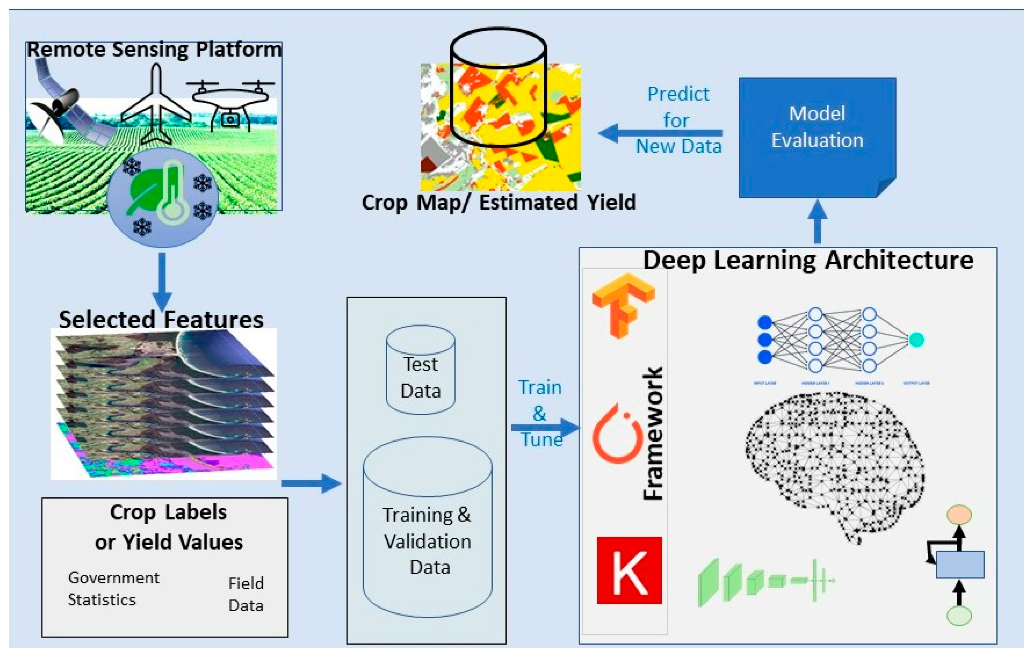
- Platform, sensor and input features of models;
- Training data used;
- Architecture used;
- Framework used to implement the architecture;
- Crop type, site, area and scale of the studies;
- Assessment criteria and performance achieved in the studies.
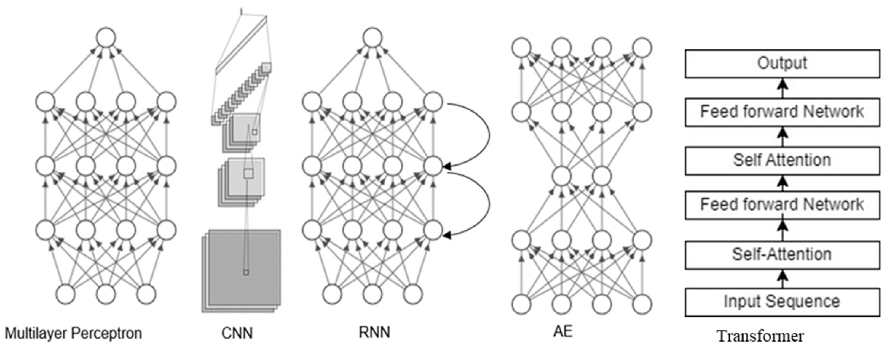
2. Overview of Deep Learning (DL)
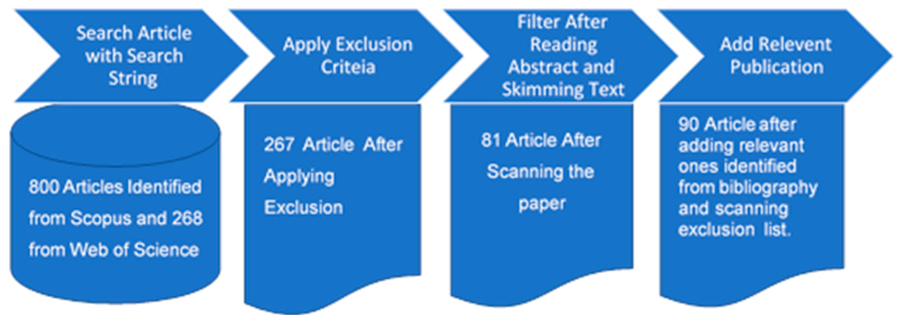
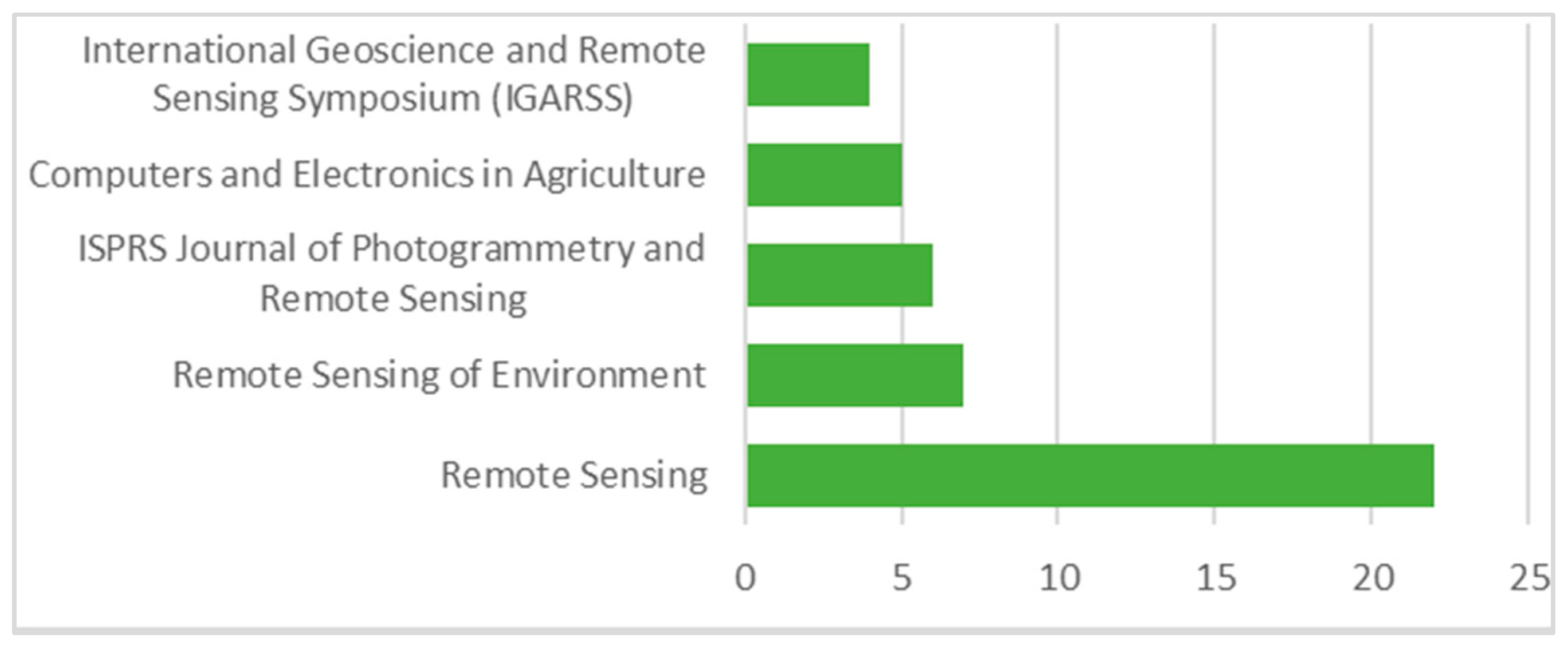
3. Literature Identification
4. Analysis of the Literature
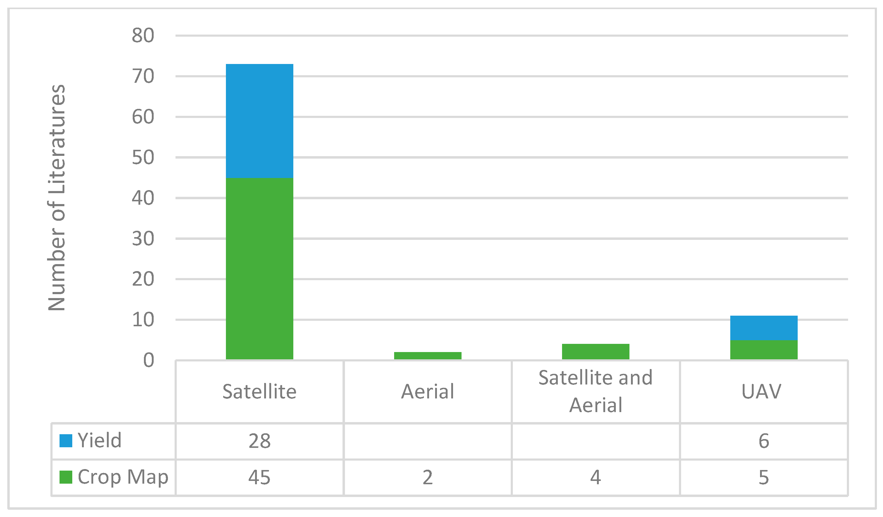
4.1. Sensors and Platforms Used
4.2. Input Features
4.3. Architecture
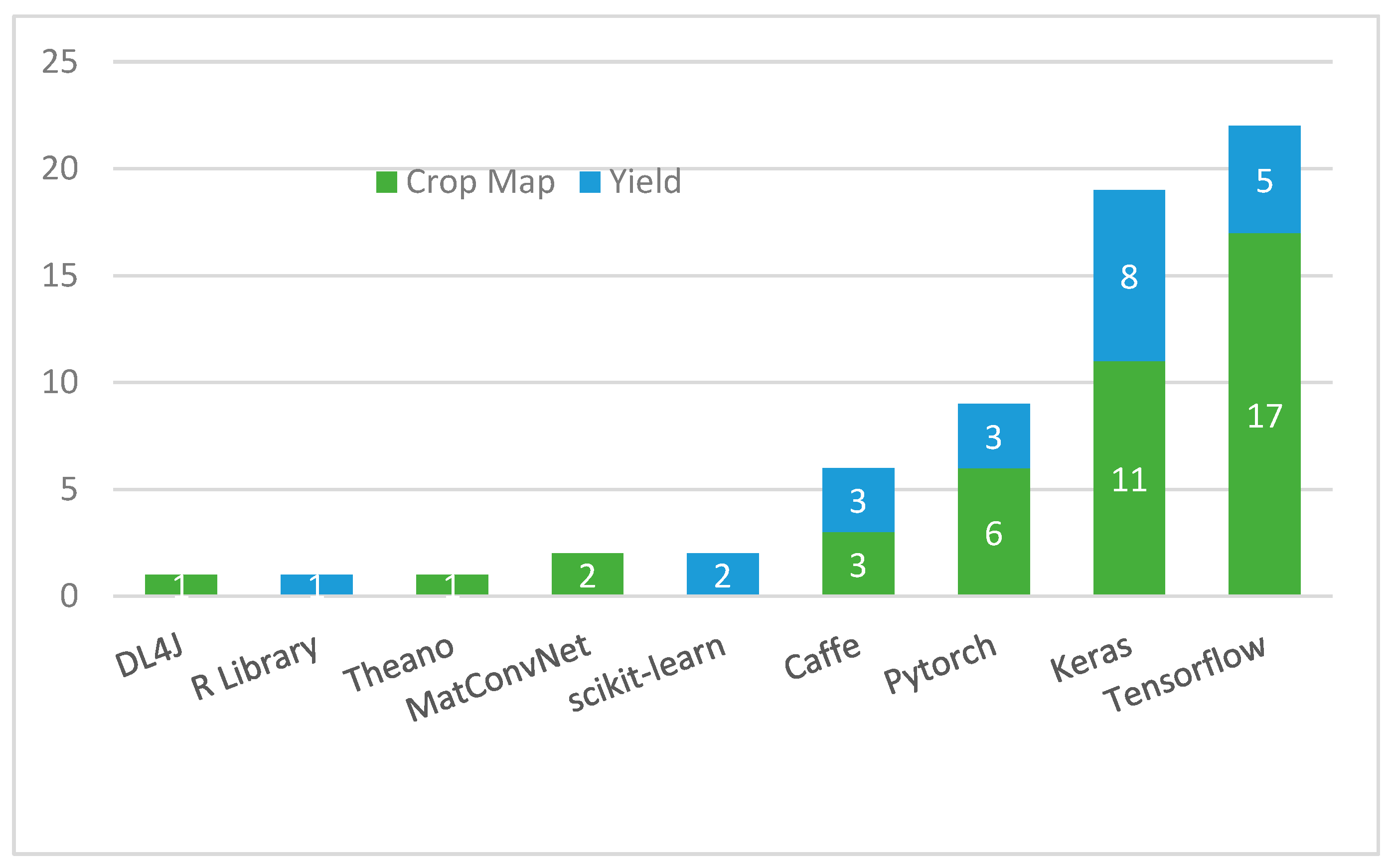
4.4. Frameworks
4.5. Crop Type
4.6. Training Data
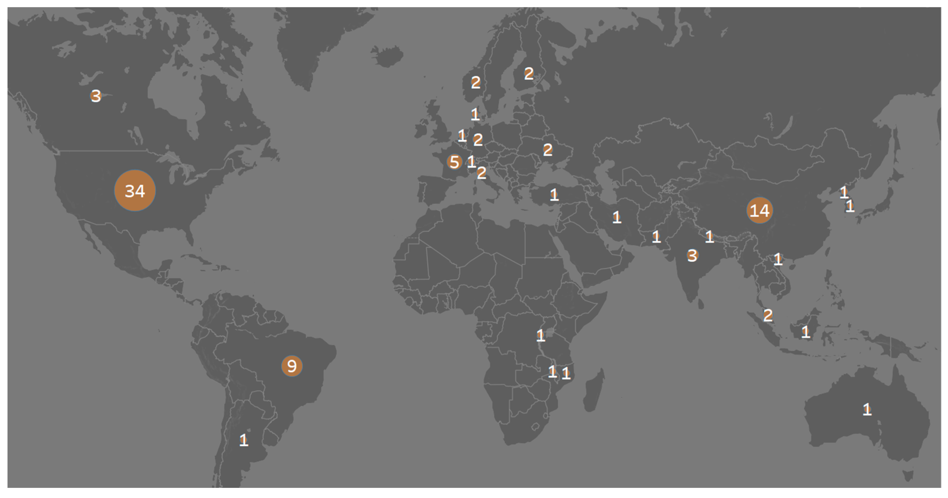
4.7. Location of Study and Area
4.8. Scale of the Output
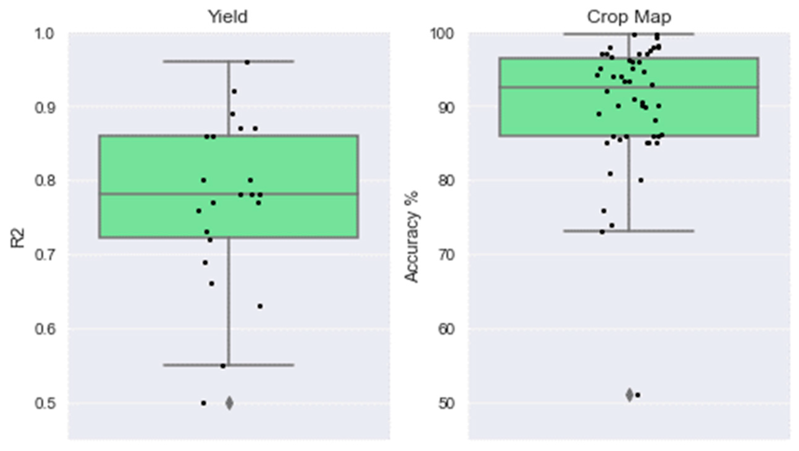
4.9. Evaluation Metrics and Performance
5. Discussion
6. Future Work
7. Conclusions
Author Contributions
Funding
Data Availability Statement
Conflicts of Interest
References
- FAO. The Future of Food and Agriculture–Trends and Challenges. Annu. Rep. 2017. Available online: https://www.fao.org/global-perspectives-studies/resources/detail/en/c/458158/ (accessed on 28 February 2023).
- Foley, J.A.; DeFries, R.; Asner, G.P.; Barford, C.; Bonan, G.; Carpenter, S.R.; Chapin, F.S.; Coe, M.T.; Daily, G.C.; Gibbs, H.K. Global Consequences of Land Use. Science 2005, 309, 570–574. [Google Scholar] [CrossRef] [PubMed] [Green Version]
- Joseph, G. Fundamentals of Remote Sensing; Universities Press: Hyderabad, India, 2005. [Google Scholar]
- Lillesand, T.; Kiefer, R.W.; Chipman, J. Remote Sensing and Image Interpretation; John Wiley & Sons: New York, NY, USA, 2015. [Google Scholar]
- Wang, A.X.; Tran, C.; Desai, N.; Lobell, D.; Ermon, S. Deep transfer learning for crop yield prediction with remote sensing data. In Proceedings of the 1st ACM SIGCAS Conference on Computing and Sustainable Societies, Menlo Park and San Jose, CA, USA, 20–22 June 2018. [Google Scholar]
- FAO. Fao’s Director-General on How to Feed the World in 2050. Popul. Dev. Rev. 2009, 35, 837–839. [Google Scholar] [CrossRef]
- Hoffman, L.A.; Etienne, X.L.; Irwin, S.H.; Colino, E.V.; Toasa, J.I. Forecast Performance of Wasde Price Projections for Us Corn. Agric. Econ. 2015, 46, 157–171. [Google Scholar] [CrossRef]
- Sherrick, B.J.; Lanoue, C.A.; Woodard, J.; Schnitkey, G.D.; Paulson, N.D. Crop Yield Distributions: Fit, Efficiency, and Performance. Agric. Financ. Rev. 2014, 74, 348–363. [Google Scholar] [CrossRef]
- Isengildina-Massa, O.; Irwin, S.H.; Good, D.L.; Gomez, J.K. The Impact of Situation and Outlook Information in Corn and Soybean Futures Markets: Evidence from Wasde Reports. J. Agric. Appl. Econ. 2008, 40, 89–103. [Google Scholar] [CrossRef] [Green Version]
- Yang, C.; Everitt, J.H.; Du, Q.; Luo, B.; Chanussot, J. Using High-Resolution Airborne and Satellite Imagery to Assess Crop Growth and Yield Variability for Precision Agriculture. Proc. IEEE 2012, 101, 582–592. [Google Scholar] [CrossRef]
- Basso, B.; Cammarano, D.; Carfagna, E. Review of crop yield forecasting methods and early warning systems. In Proceedings of the First Meeting of the Scientific Advisory Committee of the Global Strategy to Improve Agricultural and Rural Statistics, FAO Headquarters, Rome, Italy, 18 July 2013; p. 19. [Google Scholar]
- Razmjooy, N.; Estrela, V.V. Applications of Image Processing and Soft Computing Systems in Agriculture; IGI Global: Hershey, PA, USA, 2019. [Google Scholar]
- Moran, M.S.; Inoue, Y.; Barnes, E. Opportunities and Limitations for Image-Based Remote Sensing in Precision Crop Management. Remote Sens. Environ. 1997, 61, 319–346. [Google Scholar] [CrossRef]
- Karthikeyan, L.; Chawla, I.; Mishra, A.K. A Review of Remote Sensing Applications in Agriculture for Food Security: Crop Growth and Yield, Irrigation, and Crop Losses. J. Hydrol. 2020, 586, 124905. [Google Scholar] [CrossRef]
- Keating, B.A.; Carberry, P.S.; Hammer, G.L.; Probert, M.E.; Robertson, M.J.; Holzworth, D.; Huth, N.I.; Hargreaves, J.N.; Meinke, H.; Hochman, Z. An Overview of Apsim, a Model Designed for Farming Systems Simulation. Eur. J. Agron. 2003, 18, 267–288. [Google Scholar] [CrossRef] [Green Version]
- Timsina, J.; Humphreys, E. Performance of Ceres-Rice and Ceres-Wheat Models in Rice–Wheat Systems: A Review. Agric. Syst. 2006, 90, 5–31. [Google Scholar] [CrossRef]
- Brisson, N.; Gary, C.; Justes, E.; Roche, R.; Mary, B.; Ripoche, D.; Zimmer, D.; Sierra, J.; Bertuzzi, P.; Burger, P. An Overview of the Crop Model Stics. Eur. J. Agron. 2003, 18, 309–332. [Google Scholar] [CrossRef]
- Launay, M.; Guerif, M. Assimilating Remote Sensing Data into a Crop Model to Improve Predictive Performance for Spatial Applications. Agric. Ecosyst. Environ. 2005, 111, 321–339. [Google Scholar] [CrossRef]
- Jin, X.; Kumar, L.; Li, Z.; Feng, H.; Xu, X.; Yang, G.; Wang, J. A Review of Data Assimilation of Remote Sensing and Crop Models. Eur. J. Agron. 2018, 92, 141–152. [Google Scholar] [CrossRef]
- Kang, Y.; Özdoğan, M. Field-Level Crop Yield Mapping with Landsat Using a Hierarchical Data Assimilation Approach. Remote Sens. Environ. 2019, 228, 144–163. [Google Scholar] [CrossRef]
- Yao, F.; Tang, Y.; Wang, P.; Zhang, J. Estimation of Maize Yield by Using a Process-Based Model and Remote Sensing Data in the Northeast China Plain. Phys. Chem. Earth Pt. A/B/C 2015, 87, 142–152. [Google Scholar] [CrossRef]
- Huang, J.; Gómez-Dans, J.L.; Huang, H.; Ma, H.; Wu, Q.; Lewis, P.E.; Liang, S.; Chen, Z.; Xue, J.-H.; Wu, Y. Assimilation of Remote Sensing into Crop Growth Models: Current Status and Perspectives. Agric. For. Meterol. 2019, 276, 107609. [Google Scholar] [CrossRef]
- Delécolle, R.; Maas, S.; Guerif, M.; Baret, F. Remote Sensing and Crop Production Models: Present Trends. ISPRS J. Photogramm. Remote Sens. 1992, 47, 145–161. [Google Scholar] [CrossRef]
- Arikan, M. Parcel Based Crop Mapping through Multi-Temporal Masking Classification of Landsat 7 Images in Karacabey, Turkey. In Proceedings of the ISPRS Symposium, Istanbul International Archives of Photogrammetry, Remote Sensing and Spatial Information Science, Istanbul, Turkey, 12–23 July 2004. [Google Scholar]
- Beltran, C.M.; Belmonte, A.C. Irrigated Crop Area Estimation Using Landsat Tm Imagery in La Mancha, Spain. Photogramm. Eng. Remote Sens. 2001, 67, 1177–1184. [Google Scholar]
- Castillejo-González, I.L.; López-Granados, F.; García-Ferrer, A.; Peña-Barragán, J.M.; Jurado-Expósito, M.; de la Orden, M.S.; González-Audicana, M. Object-and Pixel-Based Analysis for Mapping Crops and Their Agro-Environmental Associated Measures Using Quickbird Imagery. Comput. Electron. Agric. 2009, 68, 207–215. [Google Scholar] [CrossRef]
- Huang, J.; Tian, L.; Liang, S.; Ma, H.; Becker-Reshef, I.; Huang, Y.; Su, W.; Zhang, X.; Zhu, D.; Wu, W. Improving Winter Wheat Yield Estimation by Assimilation of the Leaf Area Index from Landsat Tm and Modis Data into the Wofost Model. Agric. For. Meterol. 2015, 204, 106–121. [Google Scholar] [CrossRef] [Green Version]
- Lobell, D.B.; Thau, D.; Seifert, C.; Engle, E.; Little, B. A Scalable Satellite-Based Crop Yield Mapper. Remote Sens. Environ. 2015, 164, 324–333. [Google Scholar] [CrossRef]
- Breiman, L. Random Forests. Mach. Learn. 2001, 45, 5–32. [Google Scholar] [CrossRef] [Green Version]
- Breiman, L.; Friedman, J.H.; Olshen, R.A.; Stone, C.J. Classification and Regression Trees; Routledge: New York, NY, USA, 2017. [Google Scholar]
- Cortes, C.; Vapnik, V. Support Vector Machine. Mach. Learn. 1995, 20, 273–297. [Google Scholar] [CrossRef]
- Ok, A.O.; Akar, O.; Gungor, O. Evaluation of Random Forest Method for Agricultural Crop Classification. Eur. J. Remote Sens. 2012, 45, 421–432. [Google Scholar] [CrossRef]
- Peña-Barragán, J.M.; Ngugi, M.K.; Plant, R.E.; Six, J. Object-Based Crop Identification Using Multiple Vegetation Indices, Textural Features and Crop Phenology. Remote Sens. Environ. 2011, 115, 1301–1316. [Google Scholar] [CrossRef]
- Feng, S.; Zhao, J.; Liu, T.; Zhang, H.; Zhang, Z.; Guo, X. Crop Type Identification and Mapping Using Machine Learning Algorithms and Sentinel-2 Time Series Data. IEEE J. Sel. Top. Appl. Earth Obs. Remote Sens. 2019, 12, 3295–3306. [Google Scholar] [CrossRef]
- Jeong, J.H.; Resop, J.P.; Mueller, N.D.; Fleisher, D.H.; Yun, K.; Butler, E.E.; Timlin, D.J.; Shim, K.-M.; Gerber, J.S.; Reddy, V.R. Random Forests for Global and Regional Crop Yield Predictions. PLoS ONE 2016, 11, e0156571. [Google Scholar] [CrossRef] [Green Version]
- Shekoofa, A.; Emam, Y.; Shekoufa, N.; Ebrahimi, M.; Ebrahimie, E. Determining the Most Important Physiological and Agronomic Traits Contributing to Maize Grain Yield through Machine Learning Algorithms: A New Avenue in Intelligent Agriculture. PLoS ONE 2014, 9, e97288. [Google Scholar] [CrossRef] [PubMed] [Green Version]
- Gandhi, N.; Armstrong, L.J.; Petkar, O.; Tripathy, A.K. Rice Crop Yield Prediction in India Using Support Vector Machines. In Proceedings of the 2016 13th International Joint Conference on Computer Science and Software Engineering (JCSSE), Khon Kaen, Thailand, 13–15 July 2016; pp. 1–5. [Google Scholar]
- Foody, G.M.; Mathur, A. Toward Intelligent Training of Supervised Image Classifications: Directing Training Data Acquisition for Svm Classification. Remote Sens. Environ. 2004, 93, 107–117. [Google Scholar] [CrossRef]
- Goodfellow, I.; Bengio, Y.; Courville, A. Deep Learning; MIT Press: Cambridge, MA, USA, 2016. [Google Scholar]
- Yuan, Q.; Shen, H.; Li, T.; Li, Z.; Li, S.; Jiang, Y.; Xu, H.; Tan, W.; Yang, Q.; Wang, J. Deep Learning in Environmental Remote Sensing: Achievements and Challenges. Remote Sens. Environ. 2020, 241, 111716. [Google Scholar] [CrossRef]
- Liang, S. Quantitative Remote Sensing of Land Surfaces; John Wiley & Sons: Hoboken, NJ, USA, 2005. [Google Scholar]
- You, J.; Li, X.; Low, M.; Lobell, D.; Ermon, S. Deep Gaussian Process for Crop Yield Prediction Based on Remote Sensing Data. In Proceedings of the Thirty-First AAAI conference on artificial intelligence, San Francisco, CA, USA, 4–9 February 2017. [Google Scholar]
- Zhang, L.; Zhang, L.; Du, B. Deep Learning for Remote Sensing Data: A Technical Tutorial on the State of the Art. IEEE Geosci. Remote Sens. Mag. 2016, 4, 22–40. [Google Scholar] [CrossRef]
- Hinton, G.E.; Osindero, S.; Teh, Y.-W. A Fast Learning Algorithm for Deep Belief Nets. Neural Comput. 2006, 18, 1527–1554. [Google Scholar] [CrossRef]
- LeCun, Y.; Bengio, Y.; Hinton, G. Deep Learning. Nature 2015, 521, 436–444. [Google Scholar] [CrossRef] [PubMed]
- Ma, L.; Liu, Y.; Zhang, X.; Ye, Y.; Yin, G.; Johnson, B.A. Deep Learning in Remote Sensing Applications: A Meta-Analysis and Review. ISPRS J. Photogramm. Remote Sens. 2019, 152, 166–177. [Google Scholar] [CrossRef]
- Kamilaris, A.; Prenafeta-Boldú, F.X. Deep Learning in Agriculture: A Survey. Comput. Electron. Agric. 2018, 147, 70–90. [Google Scholar] [CrossRef] [Green Version]
- Weiss, M.; Jacob, F.; Duveiller, G. Remote Sensing for Agricultural Applications: A Meta-Review. Remote Sens. Environ. 2020, 236, 111402. [Google Scholar] [CrossRef]
- Khan, M.J.; Khan, H.S.; Yousaf, A.; Khurshid, K.; Abbas, A. Modern Trends in Hyperspectral Image Analysis: A Review. IEEE Access 2018, 6, 14118–14129. [Google Scholar] [CrossRef]
- Cheng, G.; Xie, X.; Han, J.; Guo, L.; Xia, G.-S. Remote Sensing Image Scene Classification Meets Deep Learning: Challenges, Methods, Benchmarks, and Opportunities. IEEE J. Sel. Top. Appl. Earth Obs. Remote Sens. 2020, 13, 3735–3756. [Google Scholar] [CrossRef]
- Van Klompenburg, T.; Kassahun, A.; Catal, C. Crop Yield Prediction Using Machine Learning: A Systematic Literature Review. Comput. Electron. Agric. 2020, 177, 105709. [Google Scholar] [CrossRef]
- Oikonomidis, A.; Catal, C.; Kassahun, A. Deep Learning for Crop Yield Prediction: A Systematic Literature Review. N. Z. J. Crop Hortic. Sci. 2022, 1–26. [Google Scholar] [CrossRef]
- Muruganantham, P.; Wibowo, S.; Grandhi, S.; Samrat, N.H.; Islam, N. A Systematic Literature Review on Crop Yield Prediction with Deep Learning and Remote Sensing. Remote Sens. 2022, 14, 1990. [Google Scholar] [CrossRef]
- Mohri, M.; Rostamizadeh, A.; Talwalkar, A. Foundations of Machine Learning; MIT Press: Cambridge, MA, USA, 2018. [Google Scholar]
- Hornik, K.; Stinchcombe, M.; White, H. Multilayer Feedforward Networks Are Universal Approximators. Neural Netw. 1989, 2, 359–366. [Google Scholar] [CrossRef]
- Mesnil, G.; Dauphin, Y.; Yao, K.; Bengio, Y.; Deng, L.; Hakkani-Tur, D.; He, X.; Heck, L.; Tur, G.; Yu, D. Using Recurrent Neural Networks for Slot Filling in Spoken Language Understanding. IEEE T. Audio Speech 2014, 23, 530–539. [Google Scholar] [CrossRef]
- Vaswani, A.; Shazeer, N.; Parmar, N.; Uszkoreit, J.; Jones, L.; Gomez, A.N.; Kaiser, Ł.; Polosukhin, I. Attention Is All You Need. Adv. Neural Inf. Process. Syst. 2017, 30, 5999–6009. [Google Scholar]
- Kramer, M.A. Nonlinear Principal Component Analysis Using Autoassociative Neural Networks. AICHE J. 1991, 37, 233–243. [Google Scholar] [CrossRef]
- Gatys, L.A.; Ecker, A.S.; Bethge, M. A Neural Algorithm of Artistic Style. arXiv 2015, arXiv:1508.06576. [Google Scholar] [CrossRef]
- LeCun, Y.; Boser, B.; Denker, J.; Henderson, D.; Howard, R.; Hubbard, W.; Jackel, L. Handwritten Digit Recognition with a Back-Propagation Network. Adv. Neural Inf. Process. Syst. 1989, 2, 396–404. [Google Scholar]
- Krizhevsky, A.; Sutskever, I.; Hinton, G.E. Imagenet Classification with Deep Convolutional Neural Networks. Adv. Neural Inf. Process. Syst. 2012, 25, 1097–1105. [Google Scholar] [CrossRef] [Green Version]
- He, K.; Zhang, X.; Ren, S.; Sun, J. Deep Residual Learning for Image Recognition. In Proceedings of the IEEE Conference on Computer Vision and Pattern Recognition, Las Vegas, NV, USA, 27–30 June 2016; pp. 770–778. [Google Scholar]
- Redmon, J.; Divvala, S.; Girshick, R.; Farhadi, A. You Only Look Once: Unified, Real-Time Object Detection. In Proceedings of the IEEE Conference on Computer Vision and Pattern Recognition, Las Vegas, NV, USA, 27–30 June 2016; pp. 779–788. [Google Scholar]
- Novikov, A.A.; Lenis, D.; Major, D.; Hladůvka, J.; Wimmer, M.; Bühler, K. Fully Convolutional Architectures for Multiclass Segmentation in Chest Radiographs. IEEE Trans. Med. Imaging 2018, 37, 1865–1876. [Google Scholar] [CrossRef] [Green Version]
- Graves, A.; Mohamed, A.-R.; Hinton, G. Speech Recognition with Deep Recurrent Neural Networks. In Proceedings of the 2013 IEEE international conference on acoustics, speech and signal processing, Vancouver, Canada, 26–31 May 2013; pp. 6645–6649. [Google Scholar]
- Selvin, S.; Vinayakumar, R.; Gopalakrishnan, E.; Menon, V.K.; Soman, K. Stock Price Prediction Using Lstm, Rnn and Cnn-Sliding Window Model. In Proceedings of the 2017 International Conference on Advances in Computing, Communications and Informatics (ICACCI), Udupi, India, 13–16 September 2017; pp. 1643–1647. [Google Scholar]
- Bengio, Y.; Simard, P.; Frasconi, P. Learning Long-Term Dependencies with Gradient Descent Is Difficult. IEEE Trans. Neural Netw. 1994, 5, 157–166. [Google Scholar] [CrossRef]
- Hochreiter, S.; Schmidhuber, J. Long Short-Term Memory. Neural Comput. 1997, 9, 1735–1780. [Google Scholar] [CrossRef]
- Cho, K.; Van Merriënboer, B.; Gulcehre, C.; Bahdanau, D.; Bougares, F.; Schwenk, H.; Bengio, Y. Learning Phrase Representations Using Rnn Encoder-Decoder for Statistical Machine Translation. arXiv 2014, arXiv:1406.1078. [Google Scholar]
- Liu, Z.; Lin, Y.; Cao, Y.; Hu, H.; Wei, Y.; Zhang, Z.; Lin, S.; Guo, B. Swin Transformer: Hierarchical Vision Transformer Using Shifted Windows. In Proceedings of the IEEE/CVF International Conference on Computer Vision, Montreal, BC, Canada, 11–17 October 2021; pp. 10012–10022. [Google Scholar]
- Dosovitskiy, A.; Beyer, L.; Kolesnikov, A.; Weissenborn, D.; Zhai, X.; Unterthiner, T.; Dehghani, M.; Minderer, M.; Heigold, G.; Gelly, S. An Image Is Worth 16x16 Words: Transformers for Image Recognition at Scale. arXiv 2020, arXiv:2010.11929. [Google Scholar]
- Maimaitijiang, M.; Sagan, V.; Sidike, P.; Hartling, S.; Esposito, F.; Fritschi, F.B. Soybean Yield Prediction from Uav Using Multimodal Data Fusion and Deep Learning. Remote Sens. Environ. 2020, 237, 111599. [Google Scholar] [CrossRef]
- Nevavuori, P.; Narra, N.; Lipping, T. Crop Yield Prediction with Deep Convolutional Neural Networks. Comput. Electron. Agric. 2019, 163, 104859. [Google Scholar] [CrossRef]
- Yang, Q.; Shi, L.; Han, J.; Zha, Y.; Zhu, P. Deep Convolutional Neural Networks for Rice Grain Yield Estimation at the Ripening Stage Using Uav-Based Remotely Sensed Images. Field Crops Res. 2019, 235, 142–153. [Google Scholar] [CrossRef]
- Tri, N.C.; Duong, H.N.; Van Hoai, T.; Van Hoa, T.; Nguyen, V.H.; Toan, N.T.; Snasel, V. A Novel Approach Based on Deep Learning Techniques and Uavs to Yield Assessment of Paddy Fields. In Proceedings of the 2017 9th International Conference on Knowledge and Systems Engineering, Hue, Vietnam, 19–21 October 2017; pp. 257–262. [Google Scholar]
- Nevavuori, P.; Narra, N.; Linna, P.; Lipping, T. Crop Yield Prediction Using Multitemporal Uav Data and Spatio-Temporal Deep Learning Models. Remote Sens. 2020, 12, 4000. [Google Scholar] [CrossRef]
- Yang, W.; Nigon, T.; Hao, Z.; Dias Paiao, G.; Fernández, F.G.; Mulla, D.; Yang, C. Estimation of Corn Yield Based on Hyperspectral Imagery and Convolutional Neural Network. Comput. Electron. Agric. 2021, 184. [Google Scholar] [CrossRef]
- Sun, J.; Di, L.; Sun, Z.; Shen, Y.; Lai, Z. County-Level Soybean Yield Prediction Using Deep Cnn-Lstm Model. Sensors 2019, 19, 4363. [Google Scholar] [CrossRef] [Green Version]
- Schwalbert, R.A.; Amado, T.; Corassa, G.; Pott, L.P.; Prasad, P.V.V.; Ciampitti, I.A. Satellite-Based Soybean Yield Forecast: Integrating Machine Learning and Weather Data for Improving Crop Yield Prediction in Southern Brazil. Agric. For. Meterol. 2020, 284, 107886. [Google Scholar] [CrossRef]
- Adrian, J.; Sagan, V.; Maimaitijiang, M. Sentinel Sar-Optical Fusion for Crop Type Mapping Using Deep Learning and Google Earth Engine. ISPRS J. Photogramm. Remote Sens. 2021, 175, 215–235. [Google Scholar] [CrossRef]
- Adão, T.; Hruška, J.; Pádua, L.; Bessa, J.; Peres, E.; Morais, R.; Sousa, J.J. Hyperspectral Imaging: A Review on Uav-Based Sensors, Data Processing and Applications for Agriculture and Forestry. Remote Sens. 2017, 9, 1110. [Google Scholar] [CrossRef] [Green Version]
- Zhong, L.; Hu, L.; Zhou, H. Deep Learning Based Multi-Temporal Crop Classification. Remote Sens. Environ. 2019, 221, 430–443. [Google Scholar] [CrossRef]
- Jiang, T.; Liu, X.; Wu, L. Method for Mapping Rice Fields in Complex Landscape Areas Based on Pre-Trained Convolutional Neural Network from Hj-1 a/B Data. ISPRS Int. J. Geo-Inf. 2018, 7, 418. [Google Scholar] [CrossRef] [Green Version]
- Seydi, S.T.; Amani, M.; Ghorbanian, A. A Dual Attention Convolutional Neural Network for Crop Classification Using Time-Series Sentinel-2 Imagery. Remote Sens. 2022, 14, 498. [Google Scholar] [CrossRef]
- Bhosle, K.; Musande, V. Evaluation of Deep Learning Cnn Model for Land Use Land Cover Classification and Crop Identification Using Hyperspectral Remote Sensing Images. J. Ind. Soc. Remote Sens. 2019, 47, 1949–1958. [Google Scholar] [CrossRef]
- Hoeser, T.; Kuenzer, C. Object Detection and Image Segmentation with Deep Learning on Earth Observation Data: A Review-Part I: Evolution and Recent Trends. Remote Sens. 2020, 12, 1667. [Google Scholar] [CrossRef]
- Li, W.; Fu, H.; Yu, L.; Cracknell, A. Deep Learning Based Oil Palm Tree Detection and Counting for High-Resolution Remote Sensing Images. Remote Sens. 2017, 9, 22. [Google Scholar] [CrossRef] [Green Version]
- Jiang, H.; Hu, H.; Zhong, R.; Xu, J.; Xu, J.; Huang, J.; Wang, S.; Ying, Y.; Lin, T. A Deep Learning Approach to Conflating Heterogeneous Geospatial Data for Corn Yield Estimation: A Case Study of the Us Corn Belt at the County Level. Glob. Chang. Biol. 2020, 26, 1754–1766. [Google Scholar] [CrossRef]
- Zhang, L.; Zhang, Z.; Luo, Y.; Cao, J.; Tao, F. Combining Optical, Fluorescence, Thermal Satellite, and Environmental Data to Predict County-Level Maize Yield in China Using Machine Learning Approaches. Remote Sens. 2020, 12, 21. [Google Scholar] [CrossRef] [Green Version]
- Cunha, R.L.F.; Silva, B.; Netto, M.A.S. A Scalable Machine Learning System for Pre-Season Agriculture Yield Forecast. In Proceedings of the IEEE 14th International Conference on eScience, Amsterdam, The Netherlands, 9 October 2018; pp. 423–430. [Google Scholar]
- Ma, Y.; Zhang, Z.; Kang, Y.; Özdoğan, M. Corn Yield Prediction and Uncertainty Analysis Based on Remotely Sensed Variables Using a Bayesian Neural Network Approach. Remote Sens. Environ. 2021, 259, 112408. [Google Scholar] [CrossRef]
- Fernandez-Beltran, R.; Baidar, T.; Kang, J.; Pla, F. Rice-Yield Prediction with Multi-Temporal Sentinel-2 Data and 3d Cnn: A Case Study in Nepal. Remote Sens. 2021, 13, 1391. [Google Scholar] [CrossRef]
- Wang, X.; Huang, J.; Feng, Q.; Yin, D. Winter Wheat Yield Prediction at County Level and Uncertainty Analysis in Main Wheat-Producing Regions of China with Deep Learning Approaches. Remote Sens. 2020, 12, 1744. [Google Scholar] [CrossRef]
- Jeong, S.; Ko, J.; Yeom, J.M. Predicting Rice Yield at Pixel Scale through Synthetic Use of Crop and Deep Learning Models with Satellite Data in South and North Korea. Sci. Total Environ. 2022, 802, 149726. [Google Scholar] [CrossRef]
- Zhang, L.; Zhang, Z.; Luo, Y.; Cao, J.; Xie, R.; Li, S. Integrating Satellite-Derived Climatic and Vegetation Indices to Predict Smallholder Maize Yield Using Deep Learning. Agric. For. Meterol. 2021, 311, 108666. [Google Scholar] [CrossRef]
- Engen, M.; Sando, E.; Sjolander, B.L.O.; Arenberg, S.; Gupta, R.; Goodwin, M. Farm-Scale Crop Yield Prediction from Multi-Temporal Data Using Deep Hybrid Neural Networks. Agronomy 2021, 11, 2576. [Google Scholar] [CrossRef]
- Khaki, S.; Pham, H.; Wang, L. Simultaneous Corn and Soybean Yield Prediction from Remote Sensing Data Using Deep Transfer Learning. Sci. Rep. 2021, 11, 11132. [Google Scholar] [CrossRef] [PubMed]
- Reed, B.C.; Brown, J.F.; VanderZee, D.; Loveland, T.R.; Merchant, J.W.; Ohlen, D.O. Measuring Phenological Variability from Satellite Imagery. J. Veg. Sci. 1994, 5, 703–714. [Google Scholar] [CrossRef]
- Xiao, X.; Boles, S.; Liu, J.; Zhuang, D.; Frolking, S.; Li, C.; Salas, W.; Moore III, B. Mapping Paddy Rice Agriculture in Southern China Using Multi-Temporal Modis Images. Remote Sens. Environ. 2005, 95, 480–492. [Google Scholar] [CrossRef]
- Vega, F.A.; Ramirez, F.C.; Saiz, M.P.; Rosua, F.O. Multi-Temporal Imaging Using an Unmanned Aerial Vehicle for Monitoring a Sunflower Crop. Biosys. Eng. 2015, 132, 19–27. [Google Scholar] [CrossRef]
- Wolanin, A.; Mateo-Garciá, G.; Camps-Valls, G.; Gómez-Chova, L.; Meroni, M.; Duveiller, G.; Liangzhi, Y.; Guanter, L. Estimating and Understanding Crop Yields with Explainable Deep Learning in the Indian Wheat Belt. Environ. Res. Lett. 2020, 15, 024019. [Google Scholar] [CrossRef]
- Tian, H.; Wang, P.; Tansey, K.; Han, D.; Zhang, J.; Zhang, S.; Li, H. A Deep Learning Framework under Attention Mechanism for Wheat Yield Estimation Using Remotely Sensed Indices in the Guanzhong Plain, Pr China. Int. J. Appl. Earth Obs. Geoinf. 2021, 102, 102375. [Google Scholar] [CrossRef]
- Xu, J.; Yang, J.; Xiong, X.; Li, H.; Huang, J.; Ting, K.; Ying, Y.; Lin, T. Towards Interpreting Multi-Temporal Deep Learning Models in Crop Mapping. Remote Sens. Environ. 2021, 264, 112599. [Google Scholar] [CrossRef]
- Kuwata, K.; Shibasaki, R. Estimating Crop Yields with Deep Learning and Remotely Sensed Data. In Proceedings of the 2015 IEEE International Geoscience and Remote Sensing Symposium (IGARSS), Milan, Italy, 26–31 July 2015; pp. 858–861. [Google Scholar]
- Nogueira, K.; Miranda, W.O.; Santos, J.A.D. Improving Spatial Feature Representation from Aerial Scenes by Using Convolutional Networks. In Proceedings of the Brazilian Symposium of Computer Graphic and Image Processing, Salvador, Brazil, 26–29 August 2015; pp. 289–296. [Google Scholar]
- Kussul, N.; Lavreniuk, M.; Skakun, S.; Shelestov, A. Deep Learning Classification of Land Cover and Crop Types Using Remote Sensing Data. IEEE Geosci. Remote Sens. Lett. 2017, 14, 778–782. [Google Scholar] [CrossRef]
- Hoeser, T.; Bachofer, F.; Kuenzer, C. Object Detection and Image Segmentation with Deep Learning on Earth Observation Data: A Review—Part Ii: Applications. Remote Sens. 2020, 12, 3053. [Google Scholar] [CrossRef]
- Csillik, O.; Cherbini, J.; Johnson, R.; Lyons, A.; Kelly, M. Identification of Citrus Trees from Unmanned Aerial Vehicle Imagery Using Convolutional Neural Networks. Drones 2018, 2, 39. [Google Scholar] [CrossRef] [Green Version]
- Li, W.; Dong, R.; Fu, H.; Yu, L. Large-Scale Oil Palm Tree Detection from High-Resolution Satellite Images Using Two-Stage Convolutional Neural Networks. Remote Sens. 2019, 11, 11. [Google Scholar] [CrossRef] [Green Version]
- Chen, S.-W.; Tao, C.-S. Polsar Image Classification Using Polarimetric-Feature-Driven Deep Convolutional Neural Network. IEEE Geosci. Remote Sens. Lett. 2018, 15, 627–631. [Google Scholar] [CrossRef]
- Szegedy, C.; Liu, W.; Jia, Y.; Sermanet, P.; Reed, S.; Anguelov, D.; Erhan, D.; Vanhoucke, V.; Rabinovich, A. Going Deeper with Convolutions. In Proceedings of the IEEE Conference on Computer Vision and Pattern Recognition, Boston, MA, USA, 7–12 June 2015; pp. 1–9. [Google Scholar]
- Ronneberger, O.; Fischer, P.; Brox, T. U-Net: Convolutional Networks for Biomedical Image Segmentation. In Proceedings of the International Conference on Medical Image Computing and Computer-Assisted Intervention, Munich, Germany, 5–9 October 2015; pp. 234–241. [Google Scholar]
- Du, Z.; Yang, J.; Ou, C.; Zhang, T. Smallholder Crop Area Mapped with a Semantic Segmentation Deep Learning Method. Remote Sens. 2019, 11, 888. [Google Scholar] [CrossRef] [Green Version]
- Saralioglu, E.; Gungor, O. Semantic Segmentation of Land Cover from High Resolution Multispectral Satellite Images by Spectral-Spatial Convolutional Neural Network. Geocarto Int. 2020, 37, 657–677. [Google Scholar] [CrossRef]
- Mullissa, A.G.; Persello, C.; Tolpekin, V. Fully Convolutional Networks for Multi-Temporal Sar Image Classification. In Proceedings of the International Geoscience and Remote Sensing Symposium (IGARSS), Valencia, Spain, 22–27 July 2018; pp. 6635–6638. [Google Scholar]
- La Rosa, L.E.C.; Feitosa, R.Q.; Happ, P.N.; Sanches, I.D.; da Costa, G.A.O.P. Combining Deep Learning and Prior Knowledge for Crop Mapping in Tropical Regions from Multitemporal Sar Image Sequences. Remote Sens. 2019, 11, 2029. [Google Scholar] [CrossRef] [Green Version]
- Chamorro Martinez, J.A.; Cué La Rosa, L.E.; Feitosa, R.Q.; Sanches, I.D.; Happ, P.N. Fully Convolutional Recurrent Networks for Multidate Crop Recognition from Multitemporal Image Sequences. ISPRS J. Photogramm. Remote Sens. 2021, 171, 188–201. [Google Scholar] [CrossRef]
- Wei, P.; Chai, D.; Lin, T.; Tang, C.; Du, M.; Huang, J. Large-Scale Rice Mapping under Different Years Based on Time-Series Sentinel-1 Images Using Deep Semantic Segmentation Model. ISPRS J. Photogramm. Remote Sens. 2021, 174, 198–214. [Google Scholar] [CrossRef]
- Chew, R.; Rineer, J.; Beach, R.; O’neil, M.; Ujeneza, N.; Lapidus, D.; Miano, T.; Hegarty-Craver, M.; Polly, J.; Temple, D.S. Deep Neural Networks and Transfer Learning for Food Crop Identification in Uav Images. Drones 2020, 4, 7. [Google Scholar] [CrossRef] [Green Version]
- Zhou, Z.; Li, S.; Shao, Y. Object-Oriented Crops Classification for Remote Sensing Images Based on Convolutional Neural Network. In Proceedings of the SPIE—The International Society for Optical Engineering, Berlin, Germany, 10–12 September 2018. [Google Scholar]
- Sun, Z.; Di, L.; Fang, H. Using Long Short-Term Memory Recurrent Neural Network in Land Cover Classification on Landsat and Cropland Data Layer Time Series. Int. J. Remote Sens. 2019, 40, 593–614. [Google Scholar] [CrossRef]
- Xu, J.; Zhu, Y.; Zhong, R.; Lin, Z.; Xu, J.; Jiang, H.; Huang, J.; Li, H.; Lin, T. Deepcropmapping: A Multi-Temporal Deep Learning Approach with Improved Spatial Generalizability for Dynamic Corn and Soybean Mapping. Remote Sens. Environ. 2020, 247, 111946. [Google Scholar] [CrossRef]
- Rußwurm, M.; Korner, M. Temporal Vegetation Modelling Using Long Short-Term Memory Networks for Crop Identification from Medium-Resolution Multi-Spectral Satellite Images. In Proceedings of the IEEE Conference on Computer Vision and Pattern Recognition Workshops, Honolulu, HI, USA, 21–26 July 2017; pp. 11–19. [Google Scholar]
- Castro, J.B.; Feitosa, R.Q.; La Rosa, L.C.; Diaz, P.A.; Sanches, I. A Comparative Analysis of Deep Learning Techniques for Sub-Tropical Crop Types Recognition from Multitemporal Optical/Sar Image Sequences. In Proceedings of the 2017 30th Sibgrapi Conference on Graphics, Patterns and Images (SIBGRAPI), Niteroi, Brazil, 17–20 October 2017; pp. 382–389. [Google Scholar]
- Lavreniuk, M.; Kussul, N.; Novikov, A. Deep Learning Crop Classification Approach Based on Sparse Coding of Time Series of Satellite Data. In Proceedings of the International Geoscience and Remote Sensing Symposium (IGARSS), Valencia, Spain, 22–27 July 2018; pp. 4812–4815. [Google Scholar]
- Ghazaryan, G.; Skakun, S.; König, S.; Rezaei, E.E.; Siebert, S.; Dubovyk, O. Crop Yield Estimation Using Multi-Source Satellite Image Series and Deep Learning. In Proceedings of the IGARSS 2020–2020 IEEE International Geoscience and Remote Sensing Symposium, Waikoloa, HI, USA, 26 September – 2 October; pp. 5163–5166.
- Zhao, S.; Liu, X.; Ding, C.; Liu, S.; Wu, C.; Wu, L. Mapping Rice Paddies in Complex Landscapes with Convolutional Neural Networks and Phenological Metrics. GISci. Remote Sens. 2020, 57, 37–48. [Google Scholar] [CrossRef]
- LeCun, Y.; Bottou, L.; Bengio, Y.; Haffner, P. Gradient-Based Learning Applied to Document Recognition. Proc. IEEE 1998, 86, 2278–2324. [Google Scholar] [CrossRef] [Green Version]
- Wang, Y.; Zhang, Z.; Feng, L.; Ma, Y.; Du, Q. A New Attention-Based Cnn Approach for Crop Mapping Using Time Series Sentinel-2 Images. Comput. Electron. Agric. 2021, 184, 106090. [Google Scholar] [CrossRef]
- Rußwurm, M.; Körner, M. Self-Attention for Raw Optical Satellite Time Series Classification. ISPRS J. Photogramm. Remote Sens. 2020, 169, 421–435. [Google Scholar] [CrossRef]
- Reedha, R.; Dericquebourg, E.; Canals, R.; Hafiane, A. Transformer Neural Network for Weed and Crop Classification of High Resolution Uav Images. Remote Sens. 2022, 14, 592. [Google Scholar] [CrossRef]
- Jia, Y.; Shelhamer, E.; Donahue, J.; Karayev, S.; Long, J.; Girshick, R.; Guadarrama, S.; Darrell, T. Caffe: Convolutional Architecture for Fast Feature Embedding. In Proceedings of the 22nd ACM international conference on Multimedia, Orlando, FL, USA, 3–7 November 2014; pp. 675–678. [Google Scholar]
- Bergstra, J.; Breuleux, O.; Bastien, F.; Lamblin, P.; Pascanu, R.; Desjardins, G.; Turian, J.; Warde-Farley, D.; Bengio, Y. Theano: A Cpu and Gpu Math Expression Compiler. In Proceedings of the Python for scientific computing conference (SciPy), Austin TX, USA, 28 June–3 July 2010; pp. 1–7. [Google Scholar]
- Abadi, M.; Barham, P.; Chen, J.; Chen, Z.; Davis, A.; Dean, J.; Devin, M.; Ghemawat, S.; Irving, G.; Isard, M. Tensorflow: A System for Large-Scale Machine Learning. In Proceedings of the 12th {USENIX} symposium on operating systems design and implementation ({OSDI} 16), Savannah, GA, USA, 2–4 November 2016; pp. 265–283. [Google Scholar]
- Paszke, A.; Gross, S.; Massa, F.; Lerer, A.; Bradbury, J.; Chanan, G.; Killeen, T.; Lin, Z.; Gimelshein, N.; Antiga, L. Pytorch: An Imperative Style, High-Performance Deep Learning Library. Adv. Neural Inf. Process. Syst. 2019, 32, 8026–8037. [Google Scholar]
- Seide, F.; Agarwal, A. Cntk: Microsoft’s Open-Source Deep-Learning Toolkit. In Proceedings of the 22nd ACM SIGKDD International Conference on Knowledge Discovery and Data Mining, New York, NY, USA, 13 August 2016; p. 2135. [Google Scholar]
- Vedaldi, A.; Lenc, K. Matconvnet: Convolutional Neural Networks for Matlab. In Proceedings of the 23rd ACM international conference on Multimedia, Brisbane, Australia, 26–30 October 2015; pp. 689–692. [Google Scholar]
- Scikit-Learn. Available online: https://scikit-learn.org/stable/index.html (accessed on 1 March 2022).
- Mu, H.; Zhou, L.; Dang, X.; Yuan, B. Winter Wheat Yield Estimation from Multitemporal Remote Sensing Images Based on Convolutional Neural Networks. In Proceedings of the 2019 10th International Workshop on the Analysis of Multitemporal Remote Sensing Images, MultiTemp 2019, Shanghai, China, 5–7 August 2019. [Google Scholar]
- Eclipse. Deeplearning4j. Available online: https://github.com/deeplearning4j (accessed on 1 February 2023).
- NASS. Usda National Agricultural Statistics Service Cropland Data Layer. Available online: https://nassgeodata.gmu.edu/CropScape (accessed on 1 November 2022).
- Wang, S.; Di Tommaso, S.; Faulkner, J.; Friedel, T.; Kennepohl, A.; Strey, R.; Lobell, D.B. Mapping Crop Types in Southeast India with Smartphone Crowdsourcing and Deep Learning. Remote Sens. 2020, 12, 2957. [Google Scholar] [CrossRef]
- Yan, Y.; Ryu, Y. Exploring Google Street View with Deep Learning for Crop Type Mapping. ISPRS J. Photogramm. Remote Sens. 2021, 171, 278–296. [Google Scholar] [CrossRef]
- Elshamli, A.; Taylor, G.W.; Berg, A.; Areibi, S. Domain Adaptation Using Representation Learning for the Classification of Remote Sensing Images. IEEE J. Sel. Top. Appl. Earth Obs. Remote Sens. 2017, 10, 4198–4209. [Google Scholar] [CrossRef]
- Wang, S.; Chen, W.; Xie, S.M.; Azzari, G.; Lobell, D.B. Weakly Supervised Deep Learning for Segmentation of Remote Sensing Imagery. Remote Sens. 2020, 12, 207. [Google Scholar] [CrossRef] [Green Version]
- Bruzzone, B. Agriculture in Africa 2021: Focus Report. Available online: https://oxfordbusinessgroup.com/blog/bernardo-bruzzone/focus-reports/agriculture-africa-2021-focus-report (accessed on 15 March 2022).
- Becker-Reshef, I.; Justice, C.; Sullivan, M.; Vermote, E.; Tucker, C.; Anyamba, A.; Small, J.; Pak, E.; Masuoka, E.; Schmaltz, J. Monitoring Global Croplands with Coarse Resolution Earth Observations: The Global Agriculture Monitoring (Glam) Project. Remote Sens. 2010, 2, 1589–1609. [Google Scholar] [CrossRef] [Green Version]
- Lobell, D.B. The Use of Satellite Data for Crop Yield Gap Analysis. Field Crops Res. 2013, 143, 56–64. [Google Scholar] [CrossRef] [Green Version]
- Scikit-Learn. Sklearn.Metrics.F1_Score. Available online: https://scikit-learn.org/stable/modules/generated/sklearn.metrics.f1_score.html (accessed on 1 March 2022).
- Wang, Y.; Zhang, Z.; Feng, L.; Du, Q.; Runge, T. Combining Multi-Source Data and Machine Learning Approaches to Predict Winter Wheat Yield in the Conterminous United States. Remote Sens. 2020, 12, 1232. [Google Scholar] [CrossRef] [Green Version]
- Cai, Y.; Guan, K.; Lobell, D.; Potgieter, A.B.; Wang, S.; Peng, J.; Xu, T.; Asseng, S.; Zhang, Y.; You, L. Integrating Satellite and Climate Data to Predict Wheat Yield in Australia Using Machine Learning Approaches. Agric. For. Meterol. 2019, 274, 144–159. [Google Scholar] [CrossRef]
- Kaufman, S.; Rosset, S.; Perlich, C.; Stitelman, O. Leakage in Data Mining: Formulation, Detection, and Avoidance. ACM Trans. Knowl. Discov. Data (TKDD) 2012, 6, 1–21. [Google Scholar] [CrossRef]
- Audebert, N.; Le Saux, B.; Lefèvre, S. Deep Learning for Classification of Hyperspectral Data: A Comparative Review. IEEE Geosci. Remote Sens. Mag. 2019, 7, 159–173. [Google Scholar] [CrossRef] [Green Version]
- Zhou, Z.-H. A Brief Introduction to Weakly Supervised Learning. Natl Sci.Rev 2018, 5, 44–53. [Google Scholar] [CrossRef] [Green Version]
- Shorten, C.; Khoshgoftaar, T.M. A Survey on Image Data Augmentation for Deep Learning. J. Big Data 2019, 6, 60. [Google Scholar] [CrossRef]
- Torrey, L.; Shavlik, J. Transfer Learning. In Handbook of Research on Machine Learning Applications and Trends: Algorithms, Methods, and Techniques; IGI Global: Hershey, PA, USA, 2010; pp. 242–264. [Google Scholar]
- Hinton, G.; Sejnowski, T.J. Unsupervised Learning: Foundations of Neural Computation; MIT Press: Cambridge, MA, USA, 1999. [Google Scholar]
- Abdar, M.; Pourpanah, F.; Hussain, S.; Rezazadegan, D.; Liu, L.; Ghavamzadeh, M.; Fieguth, P.; Cao, X.; Khosravi, A.; Acharya, U.R. A Review of Uncertainty Quantification in Deep Learning: Techniques, Applications and Challenges. Inform. Fusion 2021, 76, 243–297. [Google Scholar] [CrossRef]
- Kendall, A.; Gal, Y. What Uncertainties Do We Need in Bayesian Deep Learning for Computer Vision? Adv. Neural Inf. Process. Syst. 2017, 30, 5580–5590. [Google Scholar]
- Ma, Y.; Zhang, Z.; Yang, H.L.; Yang, Z. An Adaptive Adversarial Domain Adaptation Approach for Corn Yield Prediction. Comput. Electron. Agric. 2021, 187, 106314. [Google Scholar] [CrossRef]
- Castelvecchi, D. Can We Open the Black Box of Ai? Nat. News 2016, 538, 20. [Google Scholar] [CrossRef] [PubMed] [Green Version]
- Gunning, D.; Stefik, M.; Choi, J.; Miller, T.; Stumpf, S.; Yang, G.-Z. Xai—Explainable Artificial Intelligence. Sci. Robot. 2019, 4, eaay7120. [Google Scholar] [CrossRef] [Green Version]


| Sensor | Attributes | Number of Usages | |
|---|---|---|---|
| Yield | Crop Map | ||
| MODIS | Multispectral sensor Spatial resolution: 250–1000 m Temporal resolution: up to a day High temporal and moderate spatial resolutions make it suitable for crop mapping and yield prediction at regional and global scales. | 22 | 0 |
| Sentinel-1 | Radar sensor Spatial resolution: 10 m Temporal resolution: ~6 days Suitable for monitor crops in cloudy weather | 0 | 14 |
| Landsat | Multispectral sensor Spatial resolution: 30 m Temporal resolution:16 days Suitable for regional/continental-scale crop mapping and regional-to-field-scale yield-prediction studies; can also be used in historical studies | 3 | 10 |
| Sentinel-2 | Multispectral sensor Spatial resolution: 10–60 m Temporal resolution: ~10 days Suitable for crop mapping in smaller fields and field-scale yield-prediction studies. | 2 | 13 |
| UAV(RGB) | Optical sensor Spatial resolution: up to centimetres Flexibility in data capture Suitable for crop mapping with precise field boundaries and field-level yield-prediction studies; limited spectral information for crop monitoring. | 2 | 4 |
| WV-3 | Multispectral sensor Spatial resolution: 1.2 m Temporal resolution: ~1 day High cost of data, suitable for mapping crops with precise field-boundary and field-scale yield-prediction studies. | 1 | 2 |
| UAV (Multispectral) | Multispectral sensor Spatial resolution: up to centimetres Flexibility in data capture Crop mapping with precise field-boundary and field-level yield-prediction studies. | 1 | 2 |
| Architecture | Number of Times Used |
|---|---|
| CNN | 52 |
| RNN | 20 |
| MLP | 6 |
| Transformer | 2 |
| AE | 4 |
| Hybrid of CNN and RNN | 14 |
| Hybrid of CNN and ML | 2 |
| Bayesian NN | 1 |
| Domain adversarial NN | 1 |
| Crop | Number of Studies | |
|---|---|---|
| Yield Prediction | Crop Classification | |
| Corn | 9 | - |
| Soybean | 9 | - |
| Corn and soybean | 2 | 3 |
| Wheat | 5 | - |
| Wheat and barley | 1 | - |
| Wheat and corn | 1 | - |
| Wheat and rapeseed | - | 1 |
| Rice | 4 | 6 |
| Multiple | 2 | 41 |
| Coffee | - | 2 |
| Oil-palm tree | - | 3 |
| Tobacco | - | 1 |
| Data Source (For Crop Mapping) | Number of Studies |
|---|---|
| Field survey | 17 |
| CDL | 13 |
| Visual interpretation (VisI) | 6 |
| Benchmark data | 5 |
| Government data (excluding CDL) | 3 |
| Crowdsourcing | 2 |
| CDL and field survey | 1 |
| Field survey and VisI | 2 |
| Data from Agricultural Company | 2 |
| Data Source (For Crop-Yield Prediction) | Number of Studies |
|---|---|
| Field data | 11 |
| Government data (excluding USDA) | 9 |
| Government data (USDA) | 11 |
| Government data (USDA) and field data | 1 |
Disclaimer/Publisher’s Note: The statements, opinions and data contained in all publications are solely those of the individual author(s) and contributor(s) and not of MDPI and/or the editor(s). MDPI and/or the editor(s) disclaim responsibility for any injury to people or property resulting from any ideas, methods, instructions or products referred to in the content. |
© 2023 by the authors. Licensee MDPI, Basel, Switzerland. This article is an open access article distributed under the terms and conditions of the Creative Commons Attribution (CC BY) license (https://creativecommons.org/licenses/by/4.0/).
Share and Cite
Joshi, A.; Pradhan, B.; Gite, S.; Chakraborty, S. Remote-Sensing Data and Deep-Learning Techniques in Crop Mapping and Yield Prediction: A Systematic Review. Remote Sens. 2023, 15, 2014. https://doi.org/10.3390/rs15082014
Joshi A, Pradhan B, Gite S, Chakraborty S. Remote-Sensing Data and Deep-Learning Techniques in Crop Mapping and Yield Prediction: A Systematic Review. Remote Sensing. 2023; 15(8):2014. https://doi.org/10.3390/rs15082014
Chicago/Turabian StyleJoshi, Abhasha, Biswajeet Pradhan, Shilpa Gite, and Subrata Chakraborty. 2023. "Remote-Sensing Data and Deep-Learning Techniques in Crop Mapping and Yield Prediction: A Systematic Review" Remote Sensing 15, no. 8: 2014. https://doi.org/10.3390/rs15082014