Article

Rice Yield Prediction in Different Growth Environments Using Unmanned Aerial Vehicle-Based Hyperspectral Imaging

1
Space Information Center, Hokkaido Information University, Ebetsu 069-8585, Japan
2
Faculty of Science, Hokkaido University, Sapporo 001-0021, Japan
3
Ornamental Plants and Vegetables Research Center, Agricultural Research Department, Hokkaido Research Organization, Takikawa 073-0026, Japan
4
Faculty of Agriculture, Tokyo University of Agriculture, Atsugi 243-0034, Japan
5
Central Agricultural Experiment Station, Agricultural Research Department, Hokkaido Research Organization, Iwamizawa 069-0365, Japan
*
Author to whom correspondence should be addressed.
Remote Sens. 2023, 15(8), 2004; https://doi.org/10.3390/rs15082004
Submission received: 14 February 2023 / Revised: 4 April 2023 / Accepted: 7 April 2023 / Published: 10 April 2023
(This article belongs to the Section Remote Sensing in Agriculture and Vegetation)

Abstract

:
There are certain growth stages and spectral regions that are optimal for obtaining a high accuracy in rice yield prediction by remote sensing. However, there is insufficient knowledge to establish a yield prediction model widely applicable for growth environments with different meteorological factors. In this study, high temporal resolution remote sensing using unmanned aerial vehicle-based hyperspectral imaging was performed to improve the yield prediction accuracy of paddy rice cultivated in different environments. The normalized difference spectral index, an index derived from canopy reflectance at any two spectral bands, was used for a simple linear regression analysis to estimate the optimum stage and spectral region for yield prediction. Although the highest prediction accuracy was obtained from the red-edge and near-infrared regions at the booting stage, the generalization performance for different growth environments was slightly higher at the heading stage than at the booting stage. The coefficient of determination and the root mean squared percentage error for the heading stage were R2 = 0.858 and RMSPE = 7.52%, and they were R2 = 0.853 and RMSPE = 9.22% for the booting stage, respectively. In addition, a correction by solar radiation was ineffective at improving the prediction accuracy. The results demonstrate the possibility of establishing regression models with a high prediction accuracy from a single remote sensing measurement at the heading stage without using meteorological data correction.

1. Introduction

Rice is the third most cultivated crop in the world after corn and wheat [1]. Global rice production more than tripled from 1961 to 2010, which is more strongly attributed to increased yields (average of 1.74% per annum) than increased cultivated areas (average of 0.49% per annum) [2]. The Asian region accounts for 91% of rice production and 87% of consumption [2]. Therefore, accurate early yield predictions for rice, especially in Asia, is important for farmers, the entire agricultural sector, and governments in terms of market prices and food security. Models for rice yield prediction vary from the conventional growth simulation model [3] to the latest deep learning model [4,5], and target spatial scales range from plant scale to global scale. Currently, the input parameters of these yield prediction models include meteorological data, such as temperature and solar radiation, and remote sensing data, such as the vegetation index, in addition to information on soil and cultivars. Among the input parameters related to the growth environment of rice, fertilizer application, cultivar type, and seedling cultivation can be modified experimentally in cultivation field trials; while meteorological parameters cannot be controlled artificially except to change transplanting dates, years, or cultivation areas. It is necessary to accumulate daily observation data for meteorological data, but it is expected that the yield can be predicted using remote sensing data with a single measurement if an appropriate time is selected [6,7].
Among remote sensing technologies, hyperspectral measurements provide the most detailed spectral information on crop growth [8]. Many paddy rice growth studies have employed hyperspectral measurements, including a portable spectrometer for recording ground data [9,10,11,12,13] and a sensor mounted on an aircraft [14,15]. Most studies aim to clarify the spectral region closely related to nitrogen and chlorophyll contents from the reflectance spectra using regression analysis or machine learning. Kawamura et al. performed a partial least squares (PLS) regression analysis on ground-based hyperspectral measurement data and paddy rice yields, and obtained the highest accuracy (R2 = 0.843) during the booting stage with the red-edge (710–740 nm) and near-infrared (830 nm) regions identified as important wavelengths for yield prediction [16]. The optimum spectral region for yield prediction is unique information acquired from hyperspectral measurements; however, this is difficult to obtain from multispectral measurements with limited spectral bands. However, frequent hyperspectral measurements on the ground or from aircrafts are difficult to obtain owing to labor and cost issues. An alternative method of multiple fields with different transplantation periods is typically used to reduce the number of hyperspectral measurements [16]. This method allows for the simultaneous measurement of different growth stages if meteorological factors are negligible compared with differences by growth stage.
Unmanned aerial vehicles (UAVs) enable the coverage of a wider area than ground-based measurements, and allow for remote sensing with a higher spatial resolution, higher frequency, and lower cost than satellite and aircraft observations. UAV-based remote sensing is expected to contribute to yield prediction models in precision agriculture [17]. Many studies use the reflectance of spectral bands obtained from UAV-based multispectral measurements and the vegetation indices derived by combining multiple bands for paddy rice yield prediction [18,19,20,21,22,23,24,25,26,27]. For example, Yuan et al. created a linear regression model to predict rice yield using 12 widely used vegetation indices obtained from the UAV multispectral imaging of paddy rice [27]. Their results showed that most of the vegetation indices correlated better with yield at the booting stage than at the heading stage. Among the vegetation indices, the normalized difference vegetation index (NDVI) and the green normalized difference vegetation index (GNDVI) were stable with little difference in prediction accuracy for different fields and stages, while the normalized difference red-edge index (NDRE) and the optimized soil adjusted vegetation index (OSAVI) had high prediction accuracy for multiple varieties and a wide range of fertilizer application rates. Frequent observations using UAV-based multispectral measurements facilitate the evaluation of yield prediction accuracy over the entire growing season after transplantation. However, accuracy may be lower when combining data from multiple years compared with data from a single year [26]. This is presumably due to annual climate differences and indicates that accuracy reduction due to different environments exceeds accuracy enhancement due to increased data. Hama et al. greatly improved yield prediction accuracy by using solar radiation data observed by meteorological satellites for correcting the vegetation index obtained by UAV-based multispectral measurements in multiple years, multiple regions, and different transplant periods [23]. However, the spectral resolution was relatively low, the center wavelength differed depending on the measurement device, and it was difficult to apply the obtained results to the dataset obtained by other devices for multispectral measurements.
Recently, a two-dimensional hyperspectral sensor became mountable on a UAV, and studies on paddy rice yield prediction based on frequent UAV-based hyperspectral measurements were reported. Wang et al. showed that the vegetation index obtained from the red-edge and near-infrared regions at the booting stage was the most predictive from single-year UAV-based hyperspectral measurements [28]. Furthermore, yield prediction accuracy was improved by combining multi-year hyperspectral measurement data with spectral information at the flowering stage [29] and obtaining textural information [30]. However, the effects of the growth environment with different meteorological factors on the yield prediction model by UAV-based multispectral measurements comparing multiple years and multiple regions are not fully known.
In this study, frequent paddy rice field observations were performed for 2 years using UAV-based hyperspectral imaging to improve yield prediction accuracy by remote sensing. The canopy reflectance spectra of paddy rice cultivated in fields at different transplanting periods each year were obtained for each plot with different fertilizer applications, cultivars, and seedling growths. A simple linear regression analysis of the vegetation indices was used to create a yield prediction model. In addition, solar radiation data were employed to improve the accuracy of the prediction model. The objectives of this study were (1) to confirm the optimum growth stage and spectral regions for yield prediction of paddy rice from high temporal resolution UAV-based hyperspectral imaging, and (2) to clarify the effect of different growth environments on the yield prediction accuracy.

2. Materials and Methods

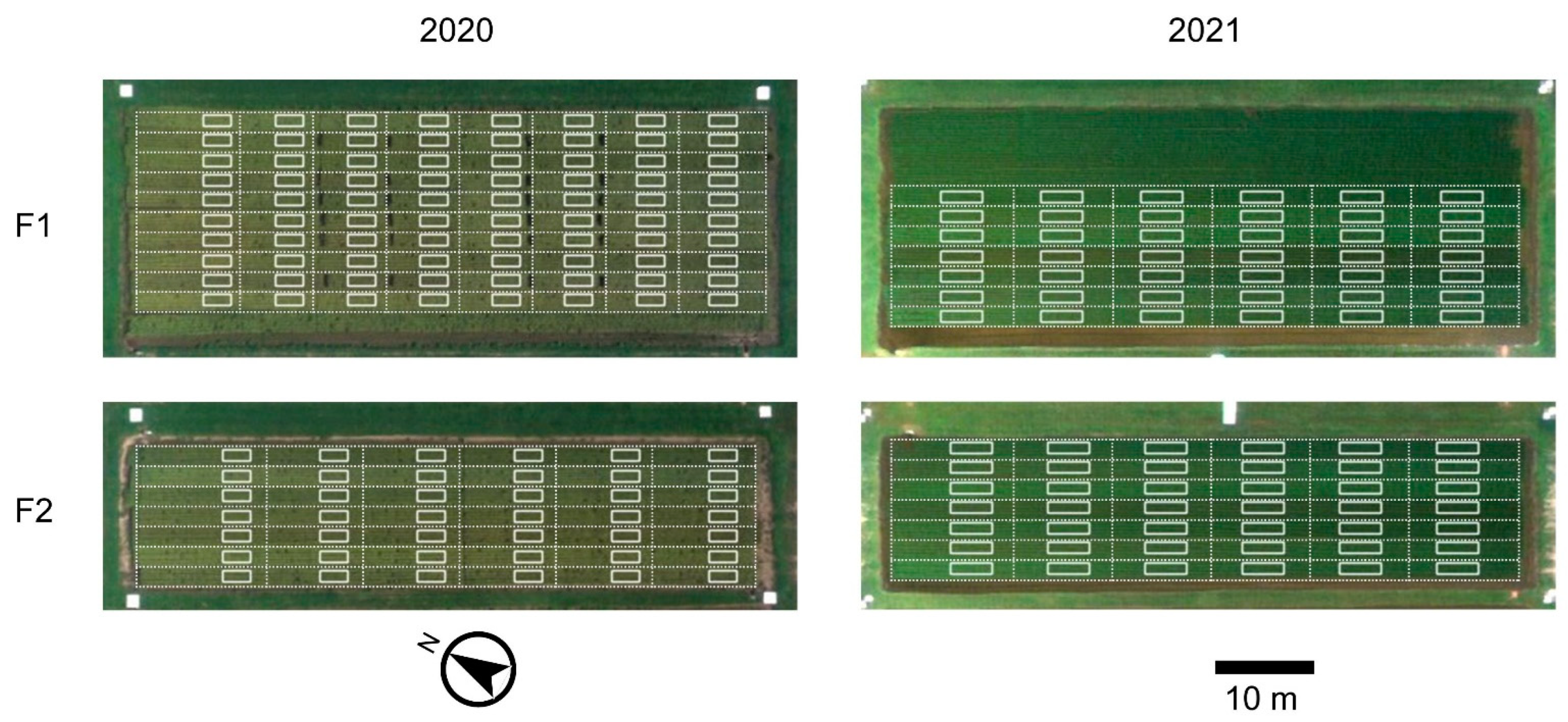
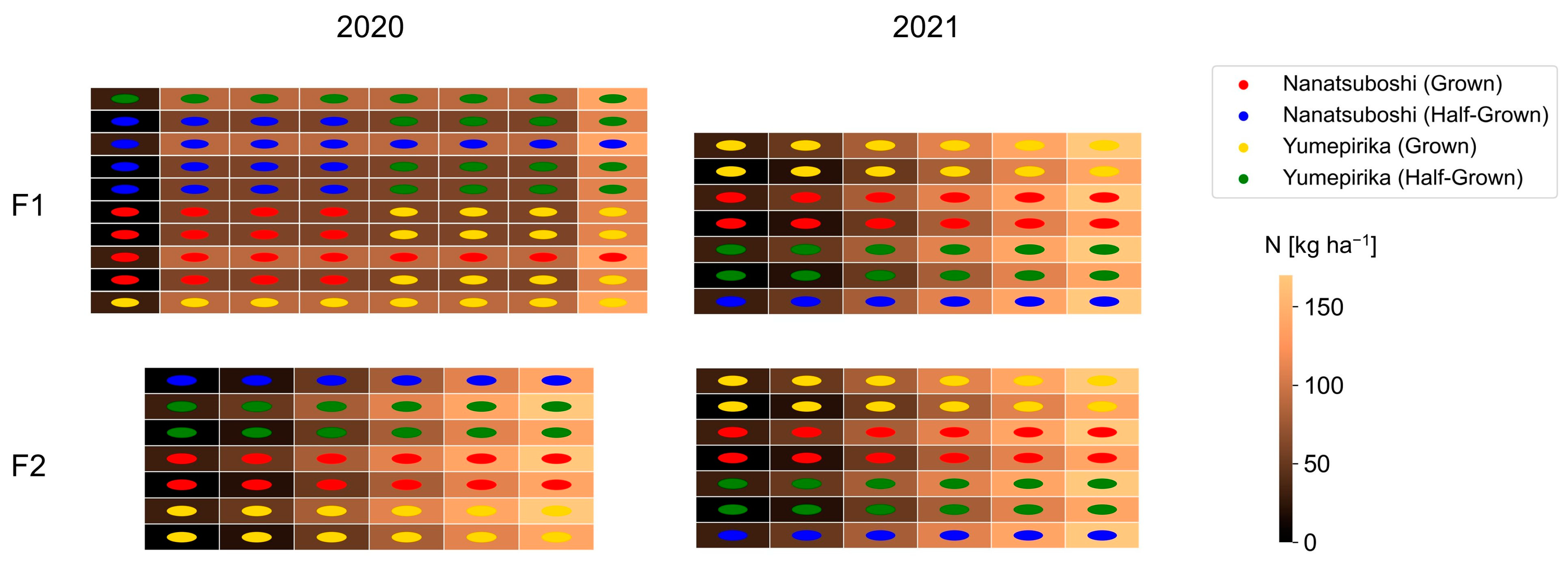
2.1. Study Site and Field Survey

The study was conducted at the cultivation technology development test field (43°10′37″N, 141°43′12″E) of the Iwamizawa Experimental Site, Central Agricultural Experiment Station, Agricultural Research Department, Hokkaido Research Organization in Iwamizawa, Hokkaido, Japan. Rice (Oryza sativa L.) seedlings were transplanted to two adjacent fields (F1 and F2; Figure 1) at intervals of 12 and 11 days in 2020 and 2021, respectively (Table 1). Each field was divided into plots with different combinations of cultivar, seedling raising, and fertilizer application (Figure 2). Each plot was 2 m wide and 8–12 m long, and the plot design varied from year to year. The two major Hokkaido cultivars were cultivated: Nanatsuboshi and Yumepirika. The seedlings were raised to 5–6 true leaves (grown seedlings) and 3–4 true leaves (half-grown). The amount of nitrogen fertilizer applied before transplantation was 0–170 kg ha−1.
The harvesting period was 100–120 days after transplanting. During the period from transplanting to harvesting, rice plants undergo three growth phases: vegetative, reproductive, and ripening. UAV-based hyperspectral imaging was focused on the reproductive and ripening phases because potential rice grain yield is primarily determined in the reproductive phase, from panicle formation to the heading stage, and ultimate yield is determined in the ripening phase after the heading stage [2]. The period between panicle formation and the heading stage is termed the booting stage.
Growth surveys were conducted for each growth stage during the cultivation period, and yields were analyzed after harvesting. The target items are the brown rice weight per unit area corresponding to the yield, the number of panicles per unit area, the number of grains per panicle, the percentage of ripened grains, and the 1000-grain weight, which are the components constituting the yield. The yield can be estimated directly by measurement or indirectly by a conventional method using the following equation from the yield components:
Y = D × N × R ÷ 100 × W ÷ 1000 ,
where Y′ is the estimated yield per unit area (g m−2), D is the number of panicles per unit area (m−2), N is the number of grains per panicle, R is the percentage of ripened grains (%), and W is the 1000-grain weight (g). The consistency between the measured yield and estimated yield was analyzed using a scatter plot (Figure 3). Although there was variation due to measurement errors, the data were generally consistent.

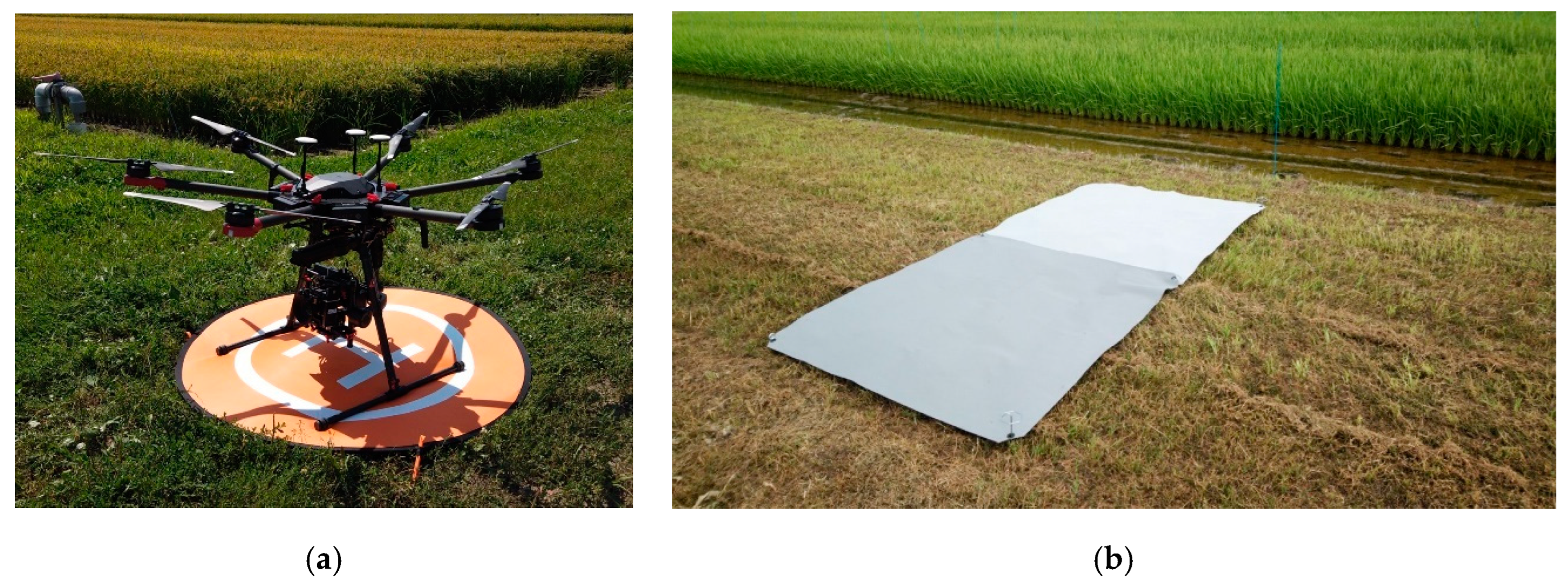
2.2. UAV-Based Hyperspectral Imaging

A sequential two-dimensional imager (Genesia Corp., Tokyo, Japan) using liquid crystal tunable filter technology was used for UAV hyperspectral imaging. Details of the imager specifications were previously described [31]. The imager can change wavelengths at a minimum interval of 1 nm from 460 to 780 nm, and the bandwidth linearly increases from 6 nm at 460 nm to 23 nm at 780 nm. Wavelength scanning of the imager was performed at 10-nm intervals and a total of 33 bands were acquired. The time required to image each band was 0.5–1 s, and approximately 30–40 s for the 33 bands. The viewing angle was 90 degrees diagonally.
This imager was attached to a gimbal RONIN-MX (SZ DJI Technology Co. Ltd., Shenzhen, China) for stability, which was mounted on a hexacopter type UAV Matrice 600 Pro (SZ DJI Technology Co. Ltd.; Figure 4a). The UAV was manually operated and stopped in the air at a height of approximately 70 m above the center of each field; the imager continuously viewed in the nadir direction. The field of view was approximately 112 × 84 m on the ground, and the spatial resolution was 0.17 m. A standard reflector with known spectral reflectance was placed on the ground in the field of view and used to convert the radiance in each band to reflectance (Figure 4b).
UAV-based hyperspectral imaging was performed 9 and 10 times from the panicle formation stage to the harvest stage in 2020 and 2021, respectively, and once every 7 days on average in each year. The measurement time was 10:30–11:30, and the combined flight time of the F1 and F2 fields was 10–15 min. The UAV cannot fly in rainy conditions or strong winds, but measurements were performed in other situations regardless of cloud coverage. However, sequences in which the solar radiation changed in a short period of time owing to cloud movement during the imaging sequence were excluded, and only the highest quality sequences were used for analysis.

2.3. Image Processing

A reflectance-based hyperspectral cube was created from the acquired hyperspectral image through four steps: radiometric correction, distortion correction, band-to-band registration, and radiance-to-reflectance conversion. In the first step, digital numbers of the pixels in each image were converted to spectral radiance values using a radiometric calibration dataset. In the second step, significant barrel distortion of each image originating from the wide FOV of the imager was removed using camera calibration parameters. In the third step, misregistration of the sequential images caused by attitude fluctuations of the UAV during the sequential imaging was corrected by band-to-band registration using feature-based matching algorithms. In the fourth step, spectral radiance values of the pixels in each image were converted to spectral reflectance values using a reflectance reference target of known spectral reflectance. The composite color image in Figure 1 was created from the hyperspectral cube. The spectral reflectance at 460–500 nm, 510–590 nm, and 600–690 nm is averaged and then assigned to the blue, green, and red channels, respectively, of the color image. Preprocessing details were previously described [31,32]. The band-to-band registration step differs from conventional preprocessing. Feature matching is applicable for band-to-band registration of forests with highly inhomogeneous brightness in captured images. However, the number of features obtained from paddy rice fields with homogeneous brightness was insufficient. In addition, the registration error sequentially increased by repeating the transformation between adjacent bands. Therefore, target markers were placed at the four outer corners of the field, and their positions were used for transformation into a single band to reduce the registration error to within 1 pixel in all bands.
Partial pixels in the plot were extracted instead of using the entire plot to derive the average reflectance of each plot (Figure 1). The entire plot was not used to avoid contamination from soil around the field and the leaves of the adjacent plots, and to avoid gaps created by sampling for growth surveys.

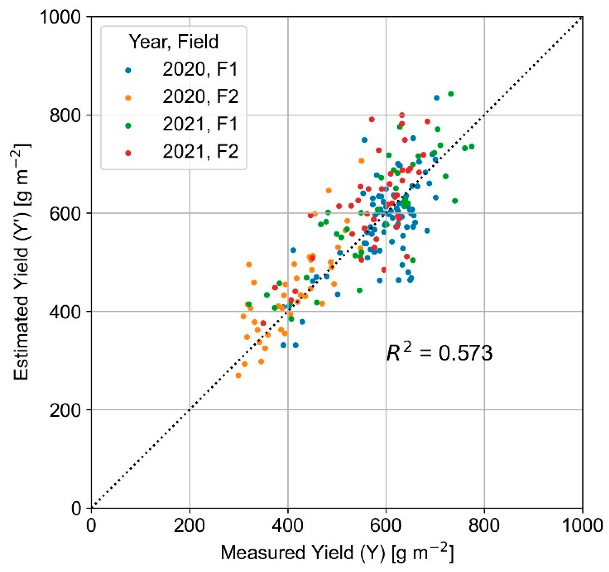
2.4. Regression Analysis

Although there are various methods for the multivariate analysis of hyperspectral data, a model using the reflectance of all bands, such as a PLS regression analysis is not always superior in terms of generalization compared with normalized spectral indices using only the optimum two bands [14,33]. This is presumably because the absolute reflectance is susceptible to sensor characteristics, measurement conditions, and atmospheric conditions, while normalization offsets these effects [33]. The hyperspectral data of this study were measured under the condition that the incident light greatly differed depending on the time and cloud cover, and the normalized spectral index was adopted. The normalized difference spectral index (NDSI) for any combination of two bands was calculated from the following equation using the spectral reflectance average for each plot:
N D S I ( λ i , λ j ) = [ R ( λ j ) R ( λ i ) ] / [ R ( λ j ) + R ( λ i ) ] ,
where R(λi) and R(λj) are the spectral reflectance values at the central wavelength λi and λj of the ith and jth spectral bands, respectively. A simple regression analysis was performed using the NDSI as an explanatory variable and a ground survey item, such as yield, as an objective variable. The prediction accuracy of the model was evaluated using the coefficient of determination R2. In addition, the root mean squared error (RMSE) and root mean squared percentage error (RMSPE) were used for a comparison of the prediction models.

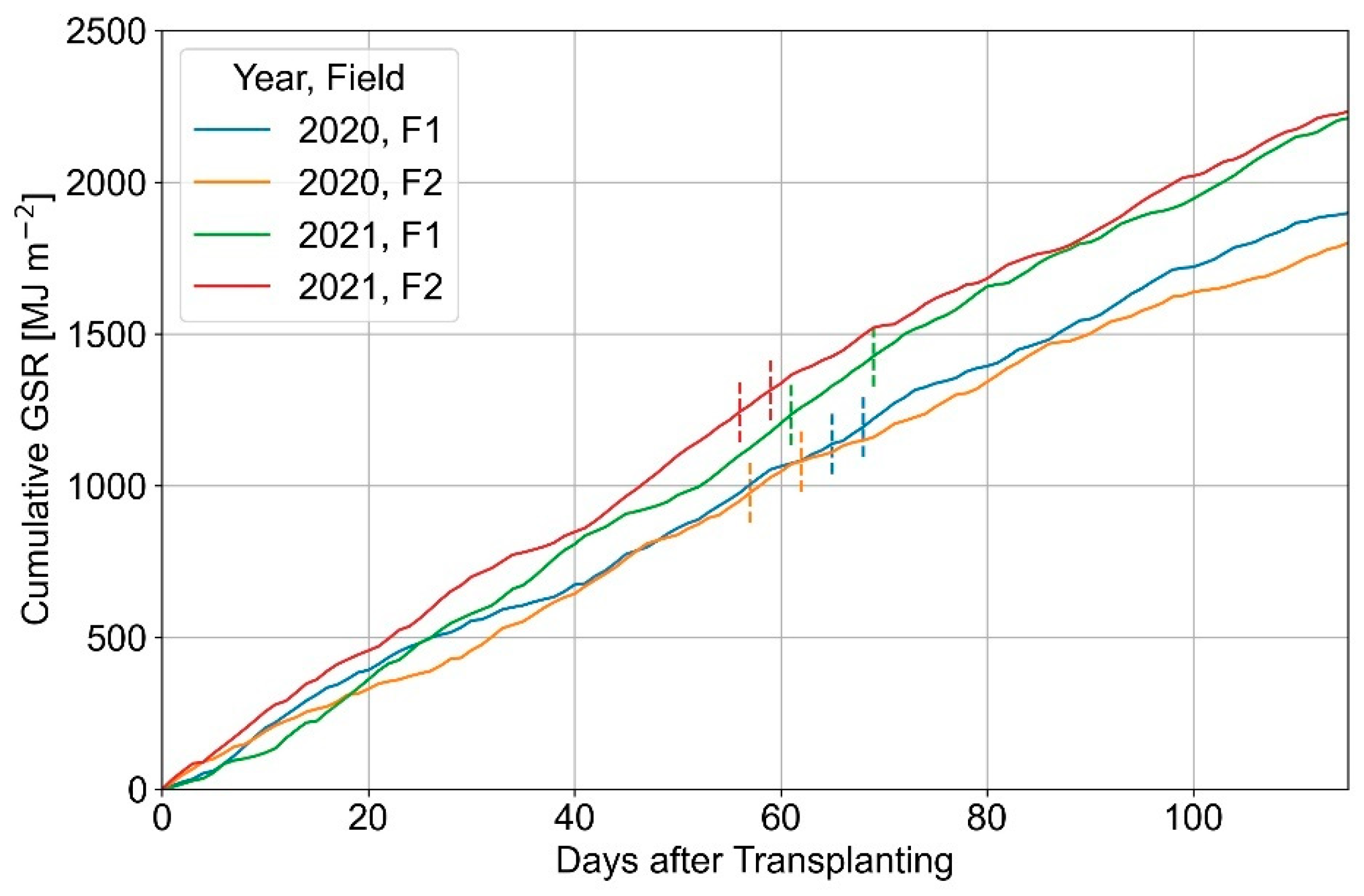
2.5. Solar Radiation Data

The solar radiation data were obtained from the Agro-Meteorological Grid Square Data of the National Agriculture and Food Research Organization [34,35]. This database provides various meteorological observation data interpolated to a 1 × 1 km grid in Japan. Daily global solar radiation (GSR, [MJ m−2 day−1]) is provided, which is the total amount of solar radiation received by the ground surface or the sum of solar radiation that arrives directly from the sun, and solar radiation that is scattered and reflected in the atmosphere. This was used to plot the time variation of GSR accumulated after transplantation (Figure 5).
Based on these data, the mean global solar radiation (mGSR) for 20 days after heading was calculated. The heading date differed depending on the plot, even in the same field; therefore, global solar radiation was integrated for each plot and averaged over 20 days:
m G S R ( i ) = 1 20 d = h ( i ) + 1 h ( i ) + 20 G S R ( d ) ,
where GSR is the daily global solar radiation, d is the number of days from the transplantation date, i is the plot number, and h(i) is the number of days from the transplantation date on the heading date in the ith plot.

3. Results

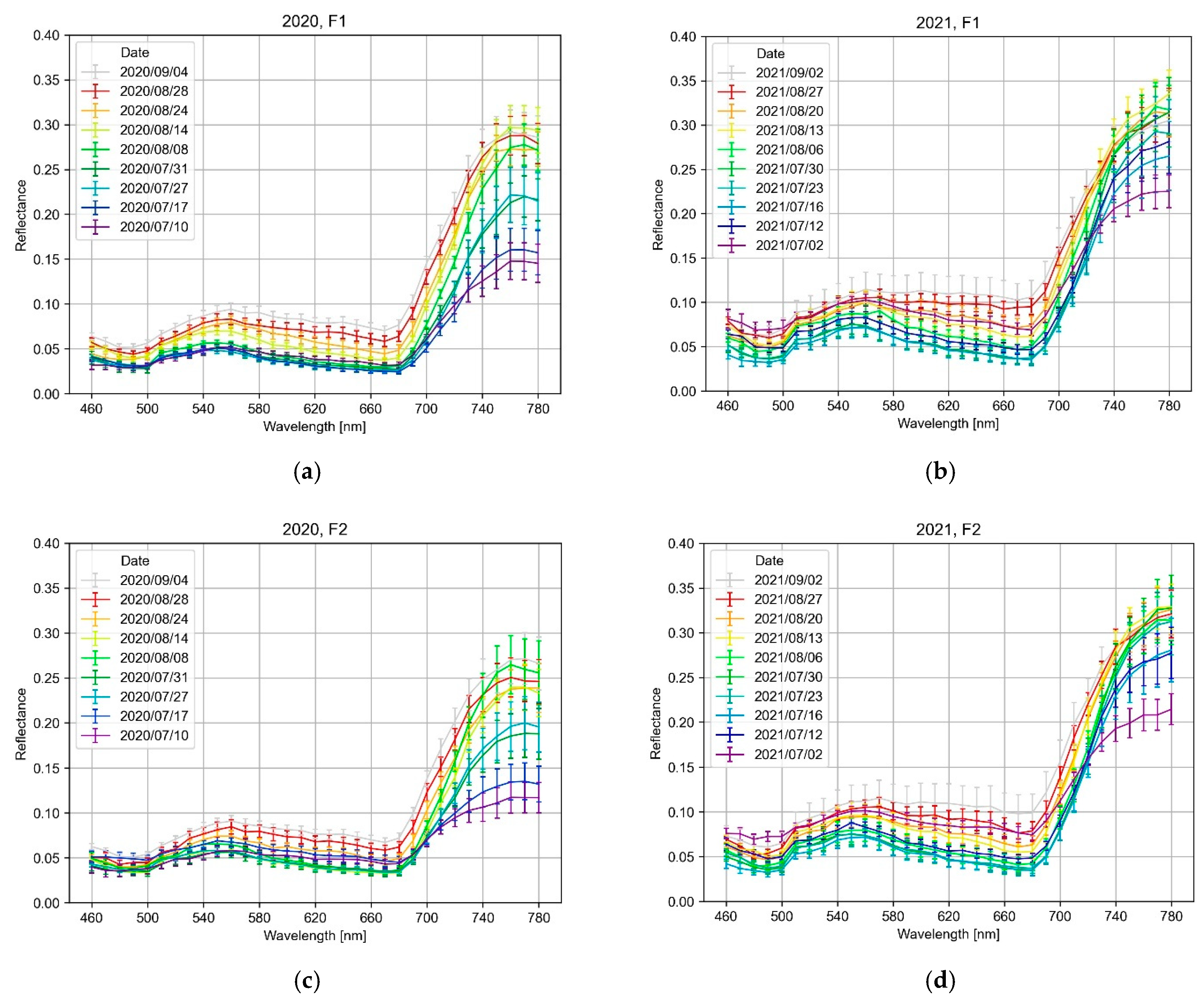
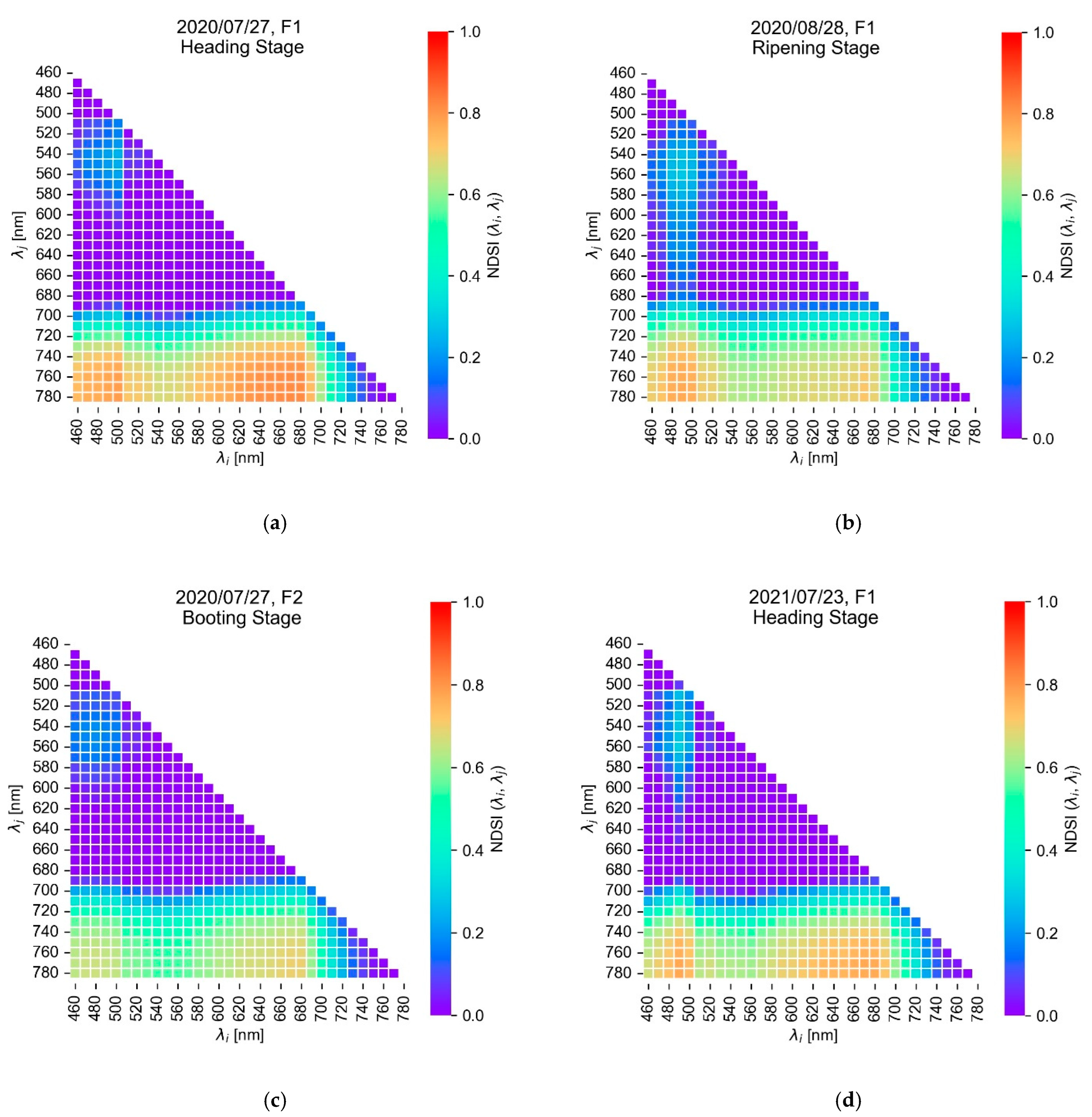
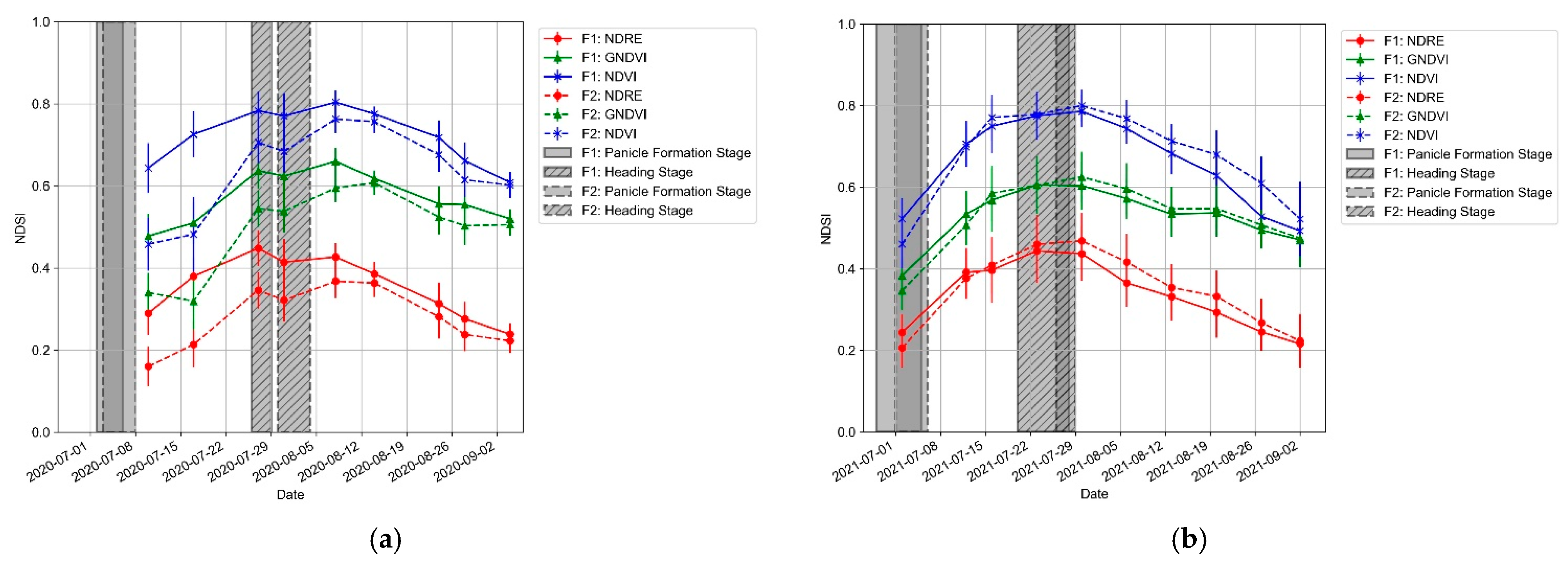
3.1. Reflectance Spectra and NDSI

The reflectance spectrum changes with paddy rice growth; however, the variation range is larger in the near-infrared region (750–780 nm; Figure 6) compared with the visible region. The reflectance in the near-infrared region rises sharply from the panicle formation stage to the heading stage, peaks at the ripening stage, and then plateaus. Meanwhile, reflectance in the visible region decreases from the panicle formation stage to the heading stage, and continuously increases after the heading stage. Reflectance in the near-infrared region is higher with early transplantation in F1 than that of F2, and is higher in 2021 than that in 2020 for the same period.
Figure 7 highlights the variability of the NDSI values at different growth stages, years, and fields for plots of the same cultivar, seedling raising, and fertilizer application (Nanatsuboshi, grown seedlings, and 140 kg ha−1). The NDSI values in the ripening stage (Figure 7b) are smaller compared with the heading stage in the combination of spectral bands where λi is the visible region and λj is the near-infrared region (Figure 7a). Meanwhile, the NDSI values of F2 (Figure 7c) with later transplantation are smaller than those of F1 (Figure 7a) even on the same day in the combination of spectral bands where λj is the near-infrared region. The NDSI values in 2021 are slightly smaller in the combination of spectral bands where λj is the near-infrared region when comparing the heading stage in 2020 (Figure 7a) and 2021 (Figure 7d). Thus, the tendency is different between the near-infrared reflectance and the NDSI using reflectance of the two spectral bands.

3.2. Yield and Yield Components

The time-series variation used the NDSI with the highest R2 value for yield and yield components in a regression analysis (Figure 8). The combination of wavelengths for the NDSI that gave the highest R2 over the entire period is not fixed, but varies by yield component, year, and field. The item with the highest R2 throughout the growth stage is the measured yield (Figure 8a), regardless of the year or field (R2 = 0.6–0.9). The estimated yield (Figure 8b) has a lower prediction accuracy (R2 ≤ 0.7) than the measured yield, and there is a large difference depending on the year and field. The number of panicles per unit area (Figure 8c) has a high coefficient of determination from the booting stage to the heading stage (R2 > 0.6), but decreases thereafter. The coefficients of determination are relatively low (R2 ≤ 0.6) for the other yield components, such as the number of grains per panicle (Figure 8d), the percentage of ripened grains (Figure 8e), and the 1000-grain weight (Figure 8f).

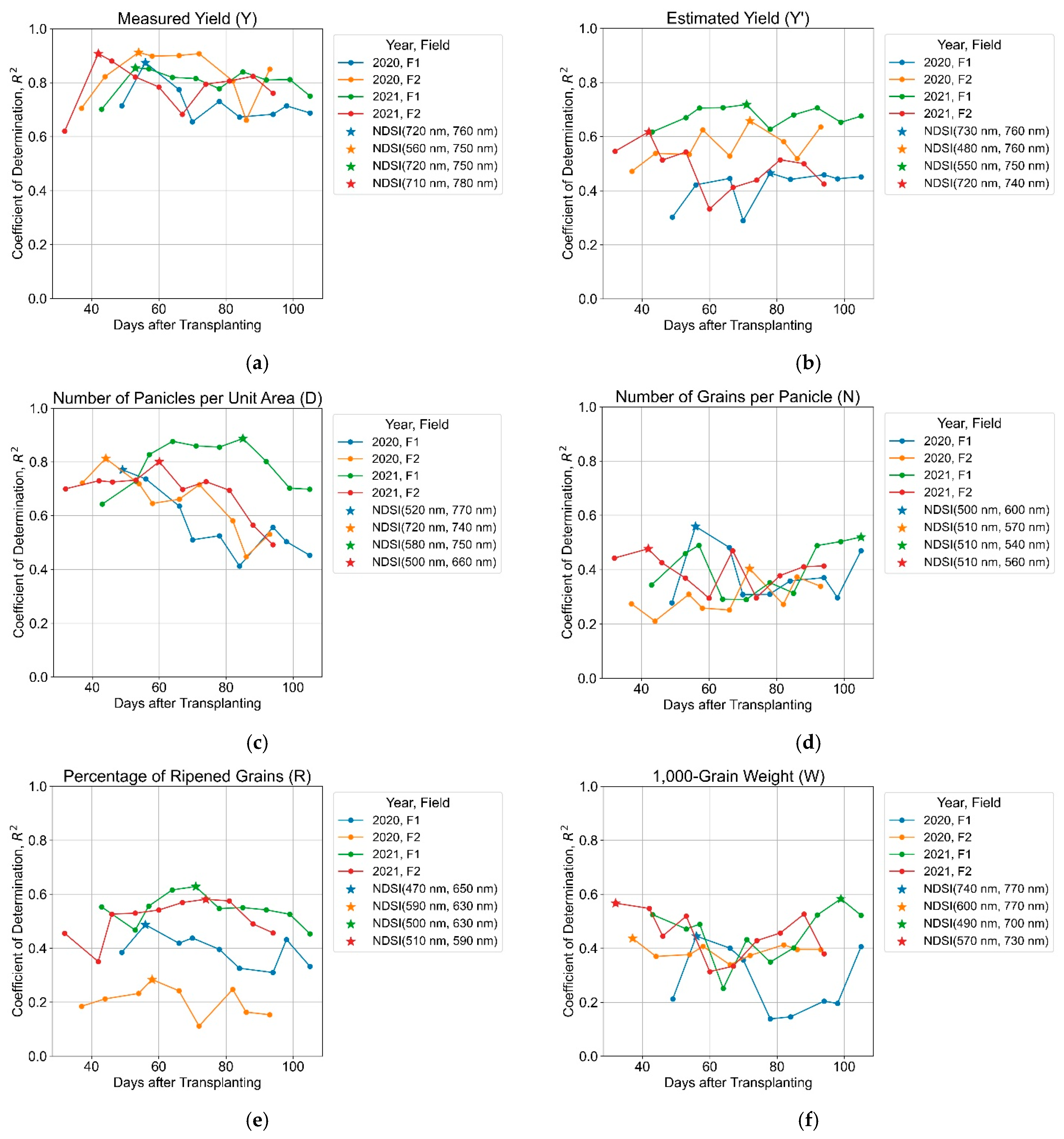
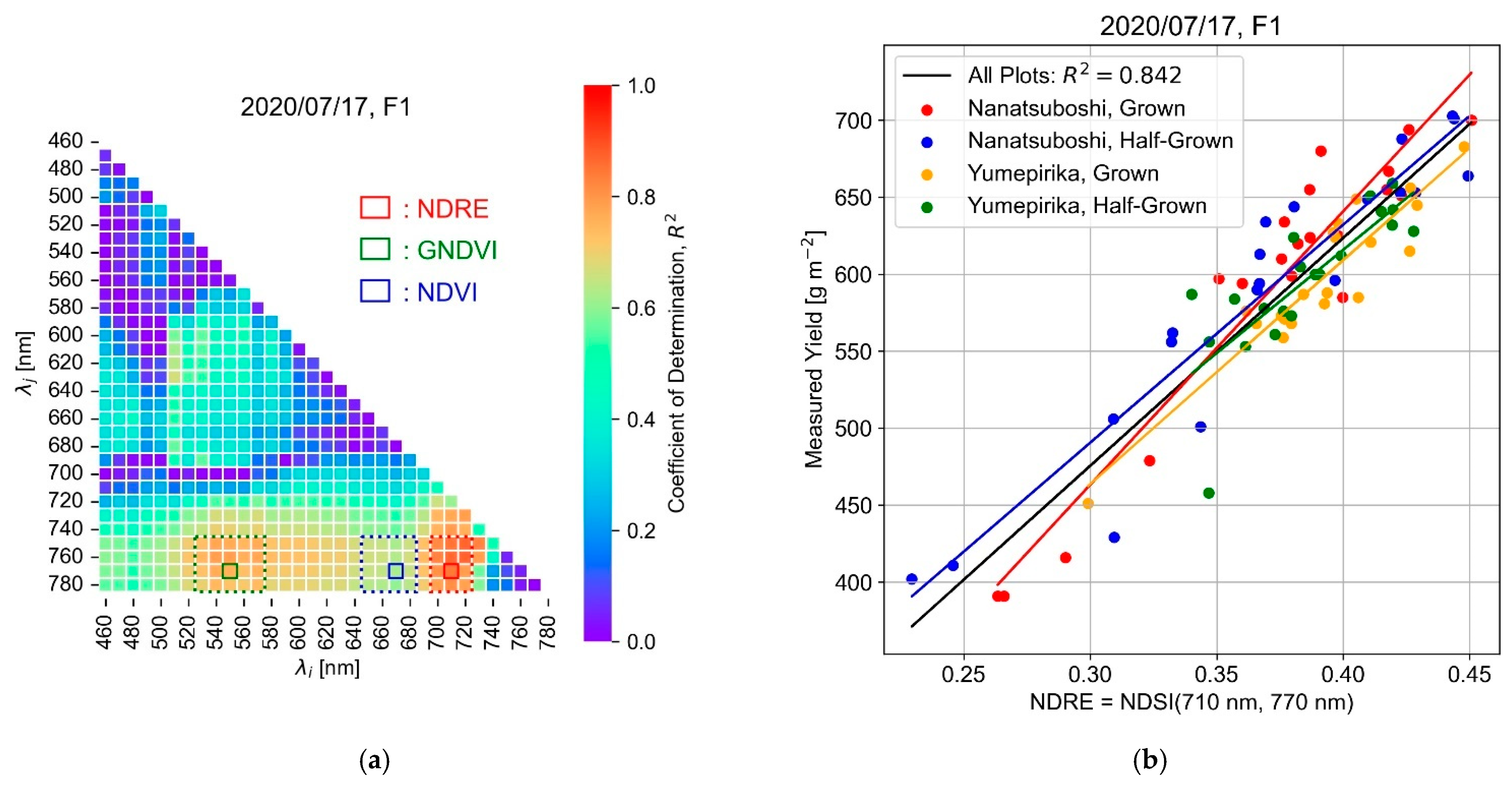
3.3. Spectral Regions with a High Prediction Accuracy

The combination of spectral bands with a high prediction accuracy for the measured yield is (1) the combination of λj = 750–780 nm in the near-infrared region and λi = 700–720 nm in the red-edge region, followed by (2) the combination of λj = 750–780 nm in the near-infrared region and λi = 530–570 nm in the green region. When these combinations are compared with the vegetation index conventionally used in multispectral observations, (1) and (2) correspond to NDRE [36] and GNDVI [37], respectively. The NDVI [38] is the most widely used vegetation index in remote sensing corresponding to the combination of λj = 750–780 nm in the near-infrared region and λi = 650–680 nm in the red region (3). However, it has a relatively lower prediction accuracy than (1) and (2). For example, a heat map of the NDSI R2 value for the measured yield on 17 July 2020 had the highest prediction accuracy in the F1 field in 2020 (Figure 9a). The R2 values for (1), (2), and (3) are in the range of 0.75–0.85, 0.65–0.75, and 0.55–0.65, respectively. The R2 variation in the regions corresponding to the three vegetation indices of NDRE, GNDVI, and NDVI on the heat map is relatively small (≤0.05). Therefore, NDRE = NDSI (710 nm, 770 nm), GNDVI = NDSI (550 nm, 770 nm), and NDVI = NDSI (670 nm, 770 nm) are defined as combinations of spectral bands that represent the three indices for simplicity. The regression lines indicating the relationship between NDRE and the measured yield are nearly identical when comparing plots with different combinations of cultivars and seedling raising (Figure 9b).

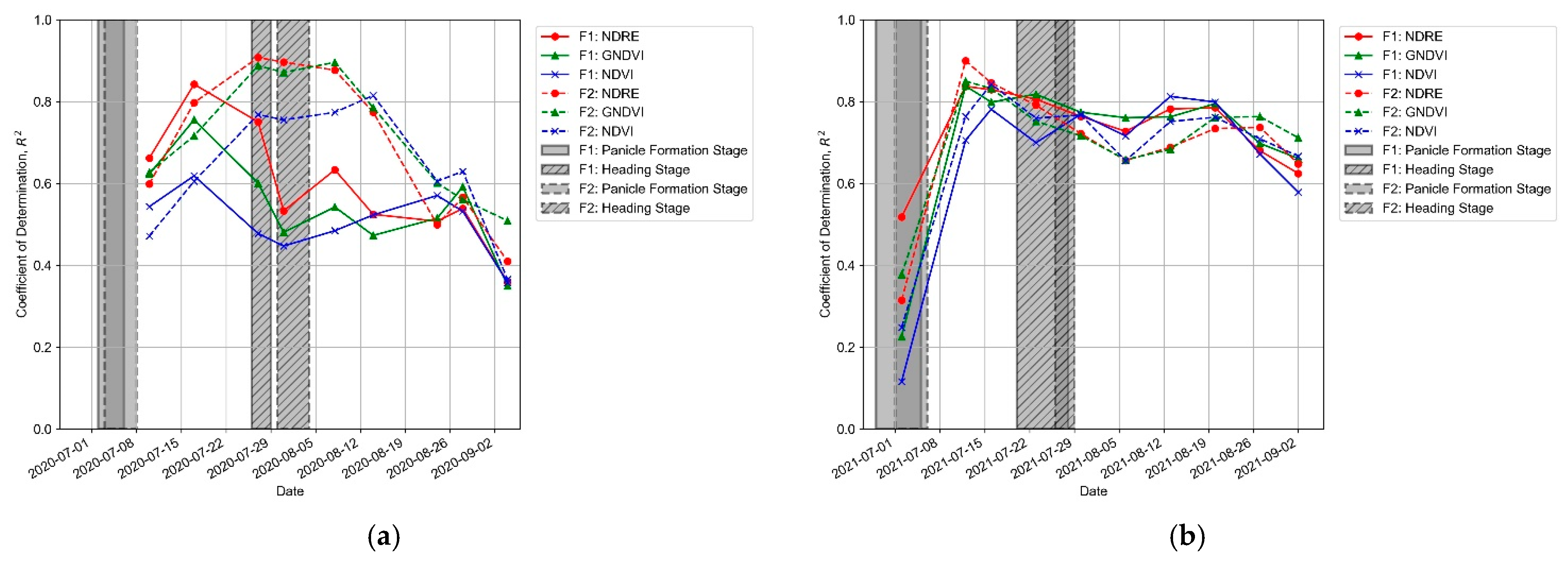
3.4. Time-Series Variation

The highest yield prediction accuracy by the NDRE and GNDVI occurs at the booting stage between the panicle formation stage and the heading stage, except for F2 in 2020 (Figure 10). The NDVI has two yield prediction accuracy peaks: the booting stage and the ripening stage, with a trough in the heading stage. The first peak is just before the F2 heading stage in 2020. However, the measurement interval near the middle of the booting stage is 10 days, and the true peak might have been during this period if the measurement was conducted.
The NDSI values are largest for the NDVI, followed by GNDVI and NDRE (Figure 11). All of the indices increase from the panicle formation stage to the heading stage, then plateau between 7 and 10 days after heading, and gradually decrease during the ripening stage.

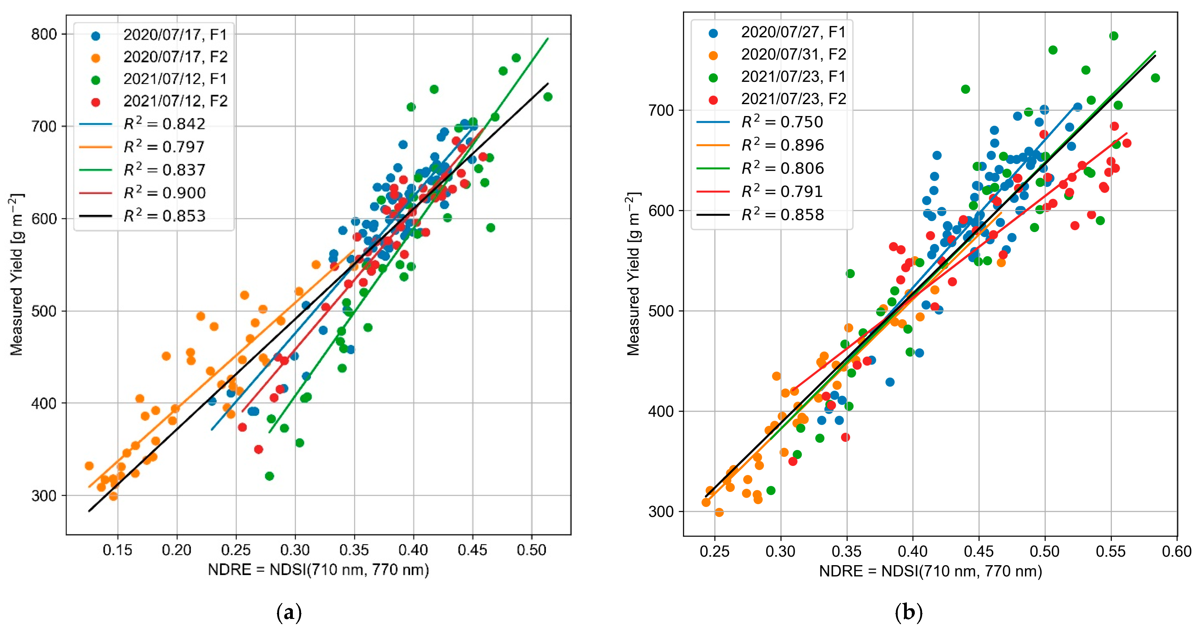
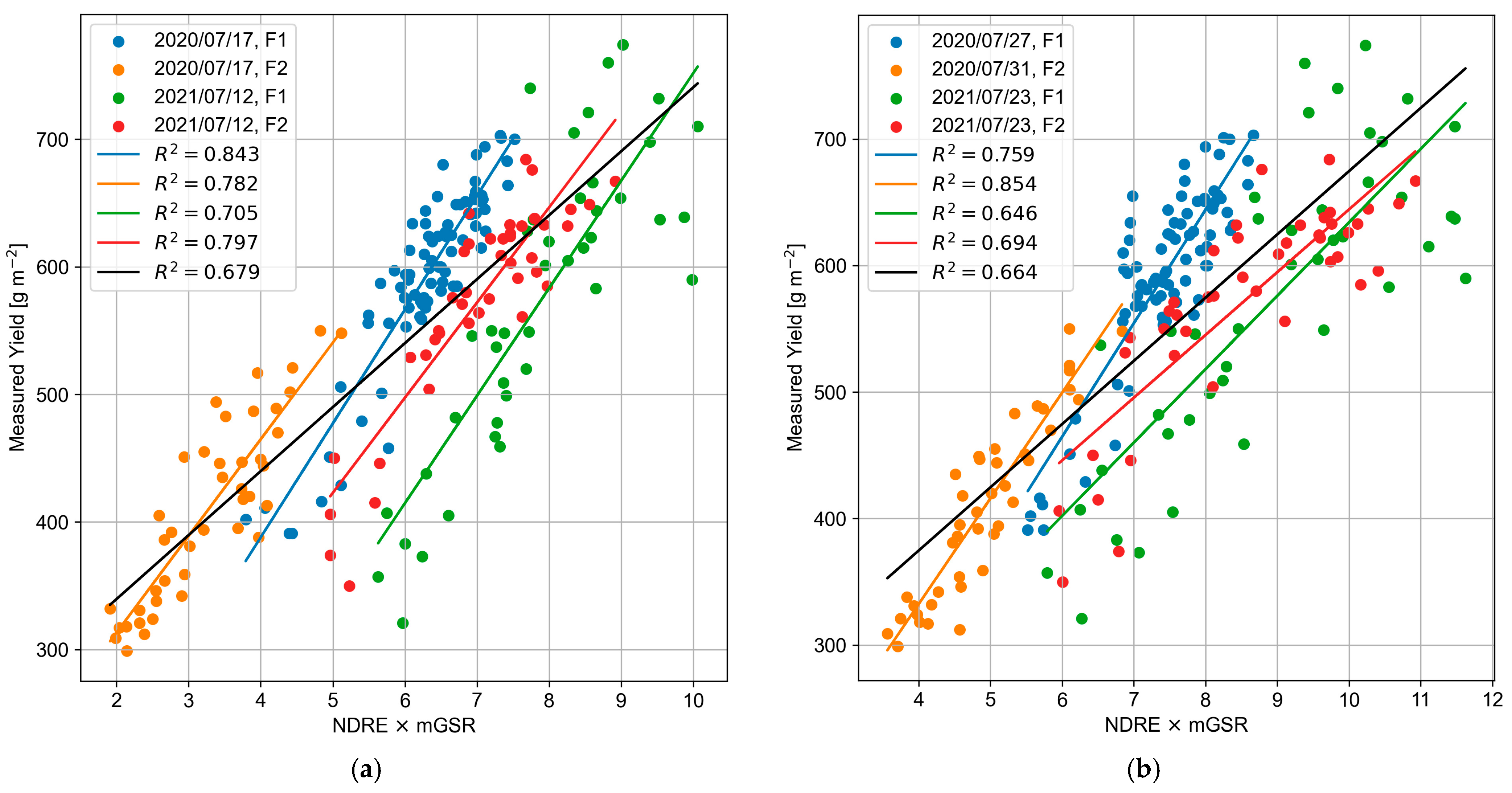
3.5. Comparison of the Different Growth Environments

A scatter plot of the NDRE and measured yields during the booting and heading stages shows that the coefficient of determination of the regression model is high for the dataset of each field in each year and all of the combined data (Figure 12). The prediction accuracy is high for the models of each field during the booting stage, but their slopes are different (Figure 12a). The prediction accuracy of each field during the heading stage is not higher than that during the booting stage, and their slopes are similar except for F2 in 2021 (Figure 12b). It should be noted that the data immediately before the heading stage were used since there are no data for the F2 heading stage in 2021.
With respect to the other performance metrics of the combined model, the RMSE and RMSPE values indicate better performance results in the heading stage compared with the booting stage (Table 2). The differences between the stages are relatively large in the RMSPE value, which reflects the percentage error between the measured and predicted yields. The slope difference between the different growth conditions in the booting stage causes large percentage errors in the lower yields.
NDRE correction using the mGSR for 20 days after heading was performed according to the method proposed by Hama et al. [23]. The NDRE was multiplied by mGSR, and the slope of the regression line changed, resulting in the data for each field in each year having almost the same slope for the booting stage (Figure 13a). However, differences in the slopes at the heading stage increase (Figure 13b). The coefficient of determination is significantly reduced in the regression model for the entire dataset at both growth stages. The effect of the correction using the mGSR is the same in the other two vegetation indices, GNDVI and NDVI (not shown here).
Finally, to visualize the utility of this yield prediction model, a predicted yield map applying the linear regression model (Table 2) for the heading stage is shown in Figure 14. For the NDRE image calculated from the reflectance in the two spectral bands at 710 and 770 nm, the predicted yield map was obtained by applying the model to the NDRE values of each pixel in the field. Compared with the plot map in Figure 1 and the fertilizer application map in Figure 2, it is clear that the predicted yields correspond to the amount of fertilizer applied in each plot. Such a visualization of the predicted yields can also be used to homogenize the yield variability in the field and improve the productivity.

4. Discussion

In this study, a regression analysis of the yield and its components was performed using the NDSI obtained from the canopy reflectance of paddy rice. The highest coefficient of determination was obtained when the measured yield was used as the objective variable. In contrast, the coefficient of determination was relatively low regarding the yield components except for the number of panicles per unit area until the heading stage. This is presumably because the number of panicles strongly depends on the amount of fertilizer applied [39]. The number of panicles is directly reflected in the vegetation indices, and is correlated with leaf and stem growth quantified by the leaf area index and chlorophyll content, which are dependent on the amount of fertilizer applied. In contrast, the tendency of the coefficient of determination for the number of panicles per unit area to decrease after the heading stage is likely to be due to the influence of the reflectance of the panicles themselves. Panicles with ripened grains have a high reflectance (up to twice as high as leaves) from the green region to the near-infrared region and have a significant effect on the canopy reflectance of paddy rice [40]. Therefore, the high values of leaves and the low values of panicles may cancel each other out in the case of the NDSI combining the visible and near-infrared regions in the NDRE, GNDVI, and NDVI. This is observed through the lower NDSI values in the ripening stage (Figure 7b) compared with the heading stage (Figure 7a) at wavelengths longer than the green region in the same plot. The fact that the estimated yield accuracy from the yield components is lower than the measured yield (Figure 8a,b) may be due to the measurement error of each yield component considering the large variability in the relationship between the measured and estimated yields (Figure 3).
Association of the NDSI with the vegetation index widely used in multispectral remote sensing showed that the prediction accuracy for the measured yield was highest for the NDRE, followed by GNDVI, and NDVI. The time-series variation showed that the NDRE and GNDVI had peaks in the booting stage, while the NDVI had two peaks, those in the booting stage and ripening stage. The highest yield prediction accuracy for the spectral bands corresponding to the NDRE during the booting stage are consistent with previous studies using hyperspectral measurements [16,28]. The peak of prediction accuracy for F2 in 2020 is close to the heading stage in the booting stage. However, there might be a true peak in the middle of the booting stage because there is a 10-day interval from the previous measurement. Although double NDVI peaks have not previously been reported, this can be attributed to the saturation effect of the NDVI. Once crop canopy cover reaches 100%, the vegetation indices begin to saturate even as crop biomass continues to increase. In the case of rice, this effect is also reported to be strong for the NDVI, but relatively weak for the GNDVI and NDRE [41]. This is because when canopy cover reaches 100%, solar radiation in the red region is strongly absorbed at the top of the canopy by chlorophyll, resulting in poor reflectance changes with increasing biomass [42]. Thus, the accuracy of rice yield prediction in the NDVI is considered to be significantly reduced at the heading stage.
In contrast to the similarity of the time-series variations, there were large year-to-year and field-to-field differences in R2 (Figure 10) and NDSI (Figure 11) values. This can be explained by differences in the growth environment: in Figure 5, the values of the cumulative GSR at the heading stage differ between 2020 and 2021, and also between the two fields in 2020. This relationship for the cumulative GSR is the same as the relationship for the R2 and NDSI values. This suggests that differences in the growth environment, including solar radiation, primarily determine the values of the R2 and NDSI. The differences in the growth environment have consequently affected the yields: the lower cumulative GSR of F2 in 2020 as compared with the other three fields corresponds to the lowest yield of F2 in 2020.
Comparison of the different growth environments of the booting stage and heading stage for the regression model used the NDRE since it had the highest prediction accuracy. The booting stage had high prediction accuracy in a specific growth environment, but generalization for different growth environments was low. This is because the NDRE value significantly changes over time owing to the high leaf and stem growth rate during the booting stage. Therefore, a slight difference in measurement time during different growing environments causes a large difference in growing conditions. In contrast, the prediction accuracy in a specific growing environment in the heading stage was mostly inferior to that in the booting stage, but generalization for different growing environments was the same or superior to the booting stage. This result implies that leaf and stem growth peak during the heading stage, and the photosynthetic products in the leaves and stems are used for the growth of panicles, resulting in peak NDRE values and decreasing time-series variation. Therefore, the heading stage is more suitable than the booting stage for yield prediction in different growing environments. This finding is a novel result that has not been reported in recent studies [24,26,28] that have analyzed yield prediction over multiple years. Furthermore, this finding can be applied to make yield predictions more robust. First, because the rice heading stage is visually obvious, it is easy to determine when to make yield predictions. Second, even if the measurement is delayed by approximately 1 week from the heading stage, the NDRE value remains stable at the plateau near its peak, minimizing the error in yield prediction. Finally, since the NDRE is a relatively common vegetation index, it can be derived with many commercially available multispectral cameras for UAVs.
Paddy rice yields are strongly correlated to the amount of solar radiation after the heading period. Hama et al. showed that yield prediction accuracy is improved by the regression analysis of the mean solar radiation for 20 days after the heading date multiplied by the NDVI at the heading stage for paddy rice in different growth environments [23]. In this study, the same analysis performed on the NDRE using the GSR showed that the prediction accuracy greatly decreased in both the booting and heading stages. A possible reason for this discrepancy is that Hama et al. analyzed paddy rice with transplantation dates that differed by up to 2 months, and a correction using the solar radiation might be required. In contrast, the transplantation dates in this study were only a maximum of 11 days apart during the different years, and so the effect of solar radiation correction was limited and dispersed compared with the quality of remote sensing data. This is clear from the fact that the prediction accuracy was reduced by the solar radiation correction for the same growth environment. This study did not consider temperature, which is another important meteorological parameter. Therefore, more advanced models considering both solar radiation and temperature may predict yields with high generalization ability for different growth environments using machine learning. However, this study demonstrates that yield prediction models can be constructed with a sufficiently high accuracy (R2 = 0.858) using a simple regression model for different growth environments without utilizing meteorological data by selecting an appropriate growth stage and spectral bands. By using multispectral satellite observation data, it may be possible to evaluate the applicability of this model to other regions, such as the tropics, where the climatic environment is very different from that of Japan. This will be the subject of future work.

5. Conclusions

The NDSI was derived from the canopy reflectance spectra of paddy rice using UAV-based hyperspectral imaging, and a yield prediction model was constructed by a simple linear regression analysis of the NDSI. The measured yield had the highest prediction accuracy in the spectral bands corresponding to the NDRE in the booting stage, which is consistent with previous studies. The generalization ability for the different growth environments in the heading stage was higher than that in the booting stage when comparing the different growth environments of the booting and heading stages for the model using the NDRE. Correction by solar radiation applied to the NDRE after the heading stage was ineffective. The main finding of this study is that a yield prediction model using the NDRE at the heading stage provided a sufficiently high accuracy (R2 = 0.858) for the different growth environments without using meteorological data. This finding implies that accurate and robust rice yield prediction is feasible through a single measurement at the heading stage using a cost-effective multispectral camera and a simple prediction model. Development of such an accessible remote sensing technology is particularly significant for rice price stabilization and food security in Asia.

Author Contributions

Methodology, software, formal analysis, investigation, data curation, writing—original draft preparation, visualization, J.K.; investigation, resources, writing—review and editing, T.N. and H.T. All authors have read and agreed to the published version of the manuscript.

Funding

This work was supported by JSPS KAKENHI (grant number JP19K06305).

Data Availability Statement

The data presented in this study are available on request from the corresponding author.

Conflicts of Interest

The authors declare no conflict of interest. The funders had no role in the design of the study; in the collection, analyses, or interpretation of data; in the writing of the manuscript, or in the decision to publish the results.

References

  1. FAOSTAT. Food and Agriculture Organization of the United Nations, Rome. Available online: http://www.fao.org/faostat/ (accessed on 7 March 2022).
  2. Maclean, J.; Hardy, B.; Hettel, G. Rice Almanac, Source Book for One of the Most Important Economic Activities on Earth, 4th ed.; IRRI: Los Baños, Philippines, 2013. [Google Scholar]
  3. Matthews, R.; Wassmann, R. Modelling the Impacts of Climate Change and Methane Emission Reductions on Rice Production: A Review. Eur. J. Agron. 2003, 19, 573–598. [Google Scholar] [CrossRef]
  4. Chlingaryan, A.; Sukkarieh, S.; Whelan, B. Machine Learning Approaches for Crop Yield Prediction and Nitrogen Status Estimation in Precision Agriculture: A Review. Comput. Electron. Agric. 2018, 151, 61–69. [Google Scholar] [CrossRef]
  5. van Klompenburg, T.; Kassahun, A.; Catal, C. Crop Yield Prediction Using Machine Learning: A Systematic Literature Review. Comput. Electron. Agric. 2020, 177, 105709. [Google Scholar] [CrossRef]
  6. Kuenzer, C.; Knauer, K. Remote Sensing of Rice Crop Areas. Int. J. Remote Sens. 2013, 34, 2101–2139. [Google Scholar] [CrossRef]
  7. Mosleh, M.K.; Hassan, Q.K.; Chowdhury, E.H. Application of Remote Sensors in Mapping Rice Area and Forecasting Its Production: A Review. Sensors 2015, 15, 769–791. [Google Scholar] [CrossRef] [Green Version]
  8. Mulla, D.J. Twenty Five Years of Remote Sensing in Precision Agriculture: Key Advances and Remaining Knowledge Gaps. Biosyst. Eng. 2013, 114, 358–371. [Google Scholar] [CrossRef]
  9. Nguyen, H.T.; Lee, B.-W. Assessment of Rice Leaf Growth and Nitrogen Status by Hyperspectral Canopy Reflectance and Partial Least Square Regression. Eur. J. Agron. 2006, 24, 349–356. [Google Scholar] [CrossRef]
  10. Inoue, Y.; Peñuelas, J.; Miyata, A.; Mano, M. Normalized Difference Spectral Indices for Estimating Photosynthetic Efficiency and Capacity at a Canopy Scale Derived from Hyperspectral and CO2 Flux Measurements in Rice. Remote Sens. Environ. 2008, 112, 156–172. [Google Scholar] [CrossRef]
  11. Xie, X.; Li, Y.X.; Li, R.; Zhang, Y.; Huo, Y.; Bao, Y.; Shen, S. Hyperspectral Characteristics and Growth Monitoring of Rice (Oryza sativa) under Asymmetric Warming. Int. J. Remote Sens. 2013, 34, 8449–8462. [Google Scholar] [CrossRef]
  12. Tan, K.; Wang, S.; Song, Y.; Liu, Y.; Gong, Z. Estimating Nitrogen Status of Rice Canopy Using Hyperspectral Reflectance Combined with BPSO-SVR in Cold Region. Chemom. Intell. Lab. Syst. 2018, 172, 68–79. [Google Scholar] [CrossRef]
  13. An, G.; Xing, M.; He, B.; Liao, C.; Huang, X.; Shang, J.; Kang, H. Using Machine Learning for Estimating Rice Chlorophyll Content from In Situ Hyperspectral Data. Remote Sens. 2020, 12, 3104. [Google Scholar] [CrossRef]
  14. Inoue, Y.; Sakaiya, E.; Zhu, Y.; Takahashi, W. Diagnostic Mapping of Canopy Nitrogen Content in Rice Based on Hyperspectral Measurements. Remote Sens. Environ. 2012, 126, 210–221. [Google Scholar] [CrossRef]
  15. Ryu, C.; Suguri, M.; Umeda, M. Multivariate Analysis of Nitrogen Content for Rice at the Heading Stage Using Reflectance of Airborne Hyperspectral Remote Sensing. Field Crops Res. 2011, 122, 214–224. [Google Scholar] [CrossRef] [Green Version]
  16. Kawamura, K.; Ikeura, H.; Phongchanmaixay, S.; Khanthavong, P. Canopy Hyperspectral Sensing of Paddy Fields at the Booting Stage and PLS Regression Can Assess Grain Yield. Remote Sens. 2018, 10, 1249. [Google Scholar] [CrossRef] [Green Version]
  17. Maes, W.H.; Steppe, K. Perspectives for Remote Sensing with Unmanned Aerial Vehicles in Precision Agriculture. Trends Plant Sci. 2019, 24, 152–164. [Google Scholar] [CrossRef] [PubMed]
  18. Stroppiana, D.; Migliazzi, M.; Chiarabini, V.; Crema, A.; Musanti, M.; Franchino, C.; Villa, P. Rice Yield Estimation Using Multispectral Data from UAV: A Preliminary Experiment in Northern Italy. In Proceedings of the 2015 IEEE International Geoscience and Remote Sensing Symposium (IGARSS), Milan, Italy, 26–31 July 2015; pp. 4664–4667. [Google Scholar] [CrossRef]
  19. Teoh, C.; Nadzim, N.M.; Shahmihaizan, M.M.; Izani, I.M.K.; Faizal, K.; Shukry, H.M. Rice Yield Estimation Using Below Cloud Remote Sensing Images Acquired by Unmanned Airborne Vehicle System. Int. J. Adv. Sci. Eng. Inf. Technol. 2016, 6, 516–519. [Google Scholar] [CrossRef] [Green Version]
  20. Zhou, X.; Zheng, H.B.; Xu, X.Q.; He, J.Y.; Ge, X.K.; Yao, X.; Cheng, T.; Zhu, Y.; Cao, W.X.; Tian, Y.C. Predicting Grain Yield in Rice Using Multi-Temporal Vegetation Indices from UAV-Based Multispectral and Digital Imagery. ISPRS J. Photogramm. Remote Sens. 2017, 130, 246–255. [Google Scholar] [CrossRef]
  21. Guan, S.; Fukami, K.; Matsunaka, H.; Okami, M.; Tanaka, R.; Nakano, H.; Sakai, T.; Nakano, K.; Ohdan, H.; Takahashi, K. Assessing Correlation of High-Resolution NDVI with Fertilizer Application Level and Yield of Rice and Wheat Crops Using Small UAVs. Remote Sens. 2019, 11, 112. [Google Scholar] [CrossRef] [Green Version]
  22. Yang, Q.; Shi, L.; Han, J.; Zha, Y.; Zhu, P. Deep Convolutional Neural Networks for Rice Grain Yield Estimation at the Ripening Stage Using UAV-Based Remotely Sensed Images. Field Crops Res. 2019, 235, 142–153. [Google Scholar] [CrossRef]
  23. Hama, A.; Tanaka, K.; Mochizuki, A.; Tsuruoka, Y.; Kondoh, A. Improving the UAV-Based Yield Estimation of Paddy Rice by Using the Solar Radiation of Geostationary Satellite Himawari-8. Hydrol. Res. Lett. 2020, 14, 56–61. [Google Scholar] [CrossRef] [Green Version]
  24. Wan, L.; Cen, H.; Zhu, J.; Zhang, J.; Zhu, Y.; Sun, D.; Du, X.; Zhai, L.; Weng, H.; Li, Y.; et al. Grain Yield Prediction of Rice Using Multi-Temporal UAV-Based RGB and Multispectral Images and Model Transfer—A Case Study of Small Farmlands in the South of China. Agric. For. Meteorol. 2020, 291, 108096. [Google Scholar] [CrossRef]
  25. Goswami, S.; Choudhary, S.S.; Chatterjee, C.; Mailapalli, D.R.; Mishra, A.; Raghuwanshi, N.S. Estimation of Nitrogen Status and Yield of Rice Crop Using Unmanned Aerial Vehicle Equipped with Multispectral Camera. J. Appl. Remote Sens. 2021, 15, 042407. [Google Scholar] [CrossRef]
  26. Kang, Y.; Nam, J.; Kim, Y.; Lee, S.; Seong, D.; Jang, S.; Ryu, C. Assessment of Regression Models for Predicting Rice Yield and Protein Content Using Unmanned Aerial Vehicle-Based Multispectral Imagery. Remote Sens. 2021, 13, 1508. [Google Scholar] [CrossRef]
  27. Yuan, N.; Gong, Y.; Fang, S.; Liu, Y.; Duan, B.; Yang, K.; Wu, X.; Zhu, R. UAV Remote Sensing Estimation of Rice Yield Based on Adaptive Spectral Endmembers and Bilinear Mixing Model. Remote Sens. 2021, 13, 2190. [Google Scholar] [CrossRef]
  28. Wang, F.; Wang, F.; Zhang, Y.; Hu, J.; Huang, J.; Xie, J. Rice Yield Estimation Using Parcel-Level Relative Spectral Variables From UAV-Based Hyperspectral Imagery. Front. Plant Sci. 2019, 10, 453. [Google Scholar] [CrossRef] [PubMed] [Green Version]
  29. Wang, F.; Yao, X.; Xie, L.; Zheng, J.; Xu, T. Rice Yield Estimation Based on Vegetation Index and Florescence Spectral Information from UAV Hyperspectral Remote Sensing. Remote Sens. 2021, 13, 3390. [Google Scholar] [CrossRef]
  30. Wang, F.; Yi, Q.; Hu, J.; Xie, L.; Yao, X.; Xu, T.; Zheng, J. Combining Spectral and Textural Information in UAV Hyperspectral Images to Estimate Rice Grain Yield. Int. J. Appl. Earth Obs. Geoinf. 2021, 102, 102397. [Google Scholar] [CrossRef]
  31. Kurihara, J.; Ishida, T.; Takahashi, Y. Unmanned Aerial Vehicle (UAV)-Based Hyperspectral Imaging System for Precision Agriculture and Forest Management. In Unmanned Aerial Vehicle: Applications in Agriculture and Environment; Avtar, R., Watanabe, T., Eds.; Springer International Publishing: Cham, Switzerland, 2020; pp. 25–38. [Google Scholar] [CrossRef]
  32. Kurihara, J.; Koo, V.-C.; Guey, C.W.; Lee, Y.P.; Abidin, H. Early Detection of Basal Stem Rot Disease in Oil Palm Tree Using Unmanned Aerial Vehicle-Based Hyperspectral Imaging. Remote Sens. 2022, 14, 799. [Google Scholar] [CrossRef]
  33. Inoue, Y.; Guérif, M.; Baret, F.; Skidmore, A.; Gitelson, A.; Schlerf, M.; Darvishzadeh, R.; Olioso, A. Simple and Robust Methods for Remote Sensing of Canopy Chlorophyll Content: A Comparative Analysis of Hyperspectral Data for Different Types of Vegetation. Plant Cell Environ. 2016, 39, 2609–2623. [Google Scholar] [CrossRef] [Green Version]
  34. Ohno, H.; Sasaki, K.; Ohara, G.; Nakazono, K. Development of grid square air temperature and precipitation data compiled from observed, forecasted, and climatic normal data. Clim. Biosph. 2016, 16, 71–79. [Google Scholar] [CrossRef] [Green Version]
  35. Kominami, Y.; Sasaki, K.; Ohno, H. User’s Manual for The Agro-Meteorological Grid Square Data, NARO Ver.4. NARO, 2019, 67p. Available online: https://www.naro.go.jp/publicity_report/publication/files/mesh_agromet_manual_v4.pdf (accessed on 7 March 2022). (In Japanese).
  36. Barnes, E.M.; Clarke, T.R.; Richards, S.E.; Colaizzi, P.D.; Haberl, J.; Kostrzewski, M.; Waller, P.; Choi, C.; Riley, E.; Thompson, T.; et al. Coincident Detection of Crop Water Stress, Nitrogen Status, and Canopy Density Using Ground-Based Multispectral Data. In Proceedings of the 5th International Conference on Precision Agriculture and other resource management, Bloomington, MN, USA, 16–19 July 2000. [Google Scholar]
  37. Gitelson, A.A.; Kaufman, Y.J.; Merzlyak, M.N. Use of a Green Channel in Remote Sensing of Global Vegetation from EOS-MODIS. Remote Sens. Environ. 1996, 58, 289–298. [Google Scholar] [CrossRef]
  38. Rouse, J.W., Jr.; Haas, R.H.; Schell, J.A.; Deering, D.W. Monitoring Vegetation Systems in the Great Plains with ERTS. NASA Spec. Publ. 1974, 351, 309–317. [Google Scholar]
  39. Fageria, N.K. Yield Physiology of Rice. J. Plant Nutr. 2007, 30, 843–879. [Google Scholar] [CrossRef]
  40. He, J.; Zhang, N.; Su, X.; Lu, J.; Yao, X.; Cheng, T.; Zhu, Y.; Cao, W.; Tian, Y. Estimating Leaf Area Index with a New Vegetation Index Considering the Influence of Rice Panicles. Remote Sens. 2019, 11, 1809. [Google Scholar] [CrossRef] [Green Version]
  41. Tsukaguchi, T.; Kobayashi, H.; Fujihara, Y.; Chono, S. Estimation of Spikelet Number per Area by UAV-Acquired Vegetation Index in Rice (Oryza sativa L.). Plant Prod. Sci. 2022, 25, 20–29. [Google Scholar] [CrossRef]
  42. Rehman, T.H.; Lundy, M.E.; Linquist, B.A. Comparative Sensitivity of Vegetation Indices Measured via Proximal and Aerial Sensors for Assessing N Status and Predicting Grain Yield in Rice Cropping Systems. Remote Sens. 2022, 14, 2770. [Google Scholar] [CrossRef]
Figure 1. Composite color images of F1 and F2 fields created from hyperspectral imaging on 28 August 2020 (ripening stage) and 16 July 2021 (booting stage). The areas surrounded by the white dotted line and white solid line are the designed plots and analyzed areas, respectively. Note that F1 in 2021 does not include all areas within the field as the designed plots.
Remotesensing 15 02004 g001
Figure 2. Cultivars, seedling raising, and nitrogen fertilizer application amount for each plot.
Remotesensing 15 02004 g002
Figure 3. Relationship between measured yield Y and estimated yield Y′. The dotted line represents Y = Y′.
Remotesensing 15 02004 g003
Figure 4. (a) Unmanned aerial vehicle (UAV) equipped with a hyperspectral imager. (b) Standard reflector installed on the ground.
Remotesensing 15 02004 g004
Figure 5. Time-series variation of the global solar radiation (GSR) accumulated after transplantation. Periods denoted by vertical dashed lines are the heading stages.
Remotesensing 15 02004 g005
Figure 6. Average reflectance spectra of the (a) F1 field in 2020, (b) F1 field in 2021, (c) F2 field in 2020, and (d) F2 field in 2021. Error bars represent the standard deviation.
Remotesensing 15 02004 g006
Figure 7. Comparison of the NDSI (normalized difference spectral index) at different growth stages, years, and fields for the same cultivar (Nanatsuboshi), seedling raising (grown seedlings), and fertilizer application (140 kg ha−1); (a) F1 field at the heading stage in 2020, (b) F1 field at the ripening stage in 2020, (c) F2 field at the booting stage in 2020, and (d) F1 field at the heading stage in 2021. The horizontal and vertical axes are the wavelengths corresponding to λi and λj of the NDSI (λi, λj), respectively.
Remotesensing 15 02004 g007
Figure 8. Time-series variations of the highest value in the coefficient of determination, R2, for prediction of (a) measured yield (Y), (b) estimated yield (Y′), (c) number of panicles per unit area (D), (d) number of grains per panicle (N), (e) percentage of ripened grains (R), and (f) 1000-grain weight (W) with respect to the number of days from transplantation. The highest R2 in the entire period and its wavelengths of the NDSI are highlighted with stars.
Remotesensing 15 02004 g008
Figure 9. (a) Heat map of the coefficient of determination for the NDSI yield in F1 on 17 July 2020. The areas surrounded by the dotted rectangles are the combination of spectral bands corresponding to the vegetation index of the NDRE (normalized difference red-edge index, red), GNDVI (green normalized difference vegetation index, green), and NDVI (normalized difference vegetation index, blue), and their representative bands (solid line). (b) Relationship between the NDRE and measured yield. The black line is the regression line from the data of all plots, and the colored line is the regression line for plots with different combinations of cultivars and seedling raising.
Remotesensing 15 02004 g009
Figure 10. Time-series variations in the coefficient of determination of each vegetation index with respect to the measured yield for each field in (a) 2020 and (b) 2021.
Remotesensing 15 02004 g010
Figure 11. Time-series variation in the NDSI values for each field in (a) 2020 and (b) 2021. Error bars represent the standard deviation of all plots.
Remotesensing 15 02004 g011
Figure 12. Relationship between the NDRE and the measured yield during the (a) booting stage and (b) heading stage.
Remotesensing 15 02004 g012
Figure 13. Relationship between the NDRE × mGSR and the measured yield during the (a) booting stage and (b) heading stage.
Remotesensing 15 02004 g013
Figure 14. (a) Composite color image of the F2 field on 23 July 2021 at the heading stage and (b) the predicted yield map superimposed on it.
Remotesensing 15 02004 g014
Table 1. Number of plots, transplanting date, panicle formation stage, and heading stage for each field in each year.
YearFieldNumber of PlotsTransplanting DatePanicle Formation StageHeading Stage
2020F180 (10 × 8)22 May 20202–6 July 202026–29 July 2020
F242 (7 × 6)3 June 20203–8 July 202030 July–4 August 2020
2021F142 (7 × 6)20 May 202128 June–5 July 202120–28 July 2021
F242 (7 × 6)31 May 20211–6 July 202126–29 July 2021
Table 2. Comparison of the simple linear regression models and their prediction performances at the booting and heading stages.
StageSlopeInterceptR2RMSE [g m−2]RMSPE [%]
Booting1193.8132.80.85342.39.22
Heading1291.50.60.85841.57.52
Disclaimer/Publisher’s Note: The statements, opinions and data contained in all publications are solely those of the individual author(s) and contributor(s) and not of MDPI and/or the editor(s). MDPI and/or the editor(s) disclaim responsibility for any injury to people or property resulting from any ideas, methods, instructions or products referred to in the content.

