

Temporal Co-Attention Guided Conditional Generative Adversarial Network for Optical Image Synthesis
Abstract
:1. Introduction
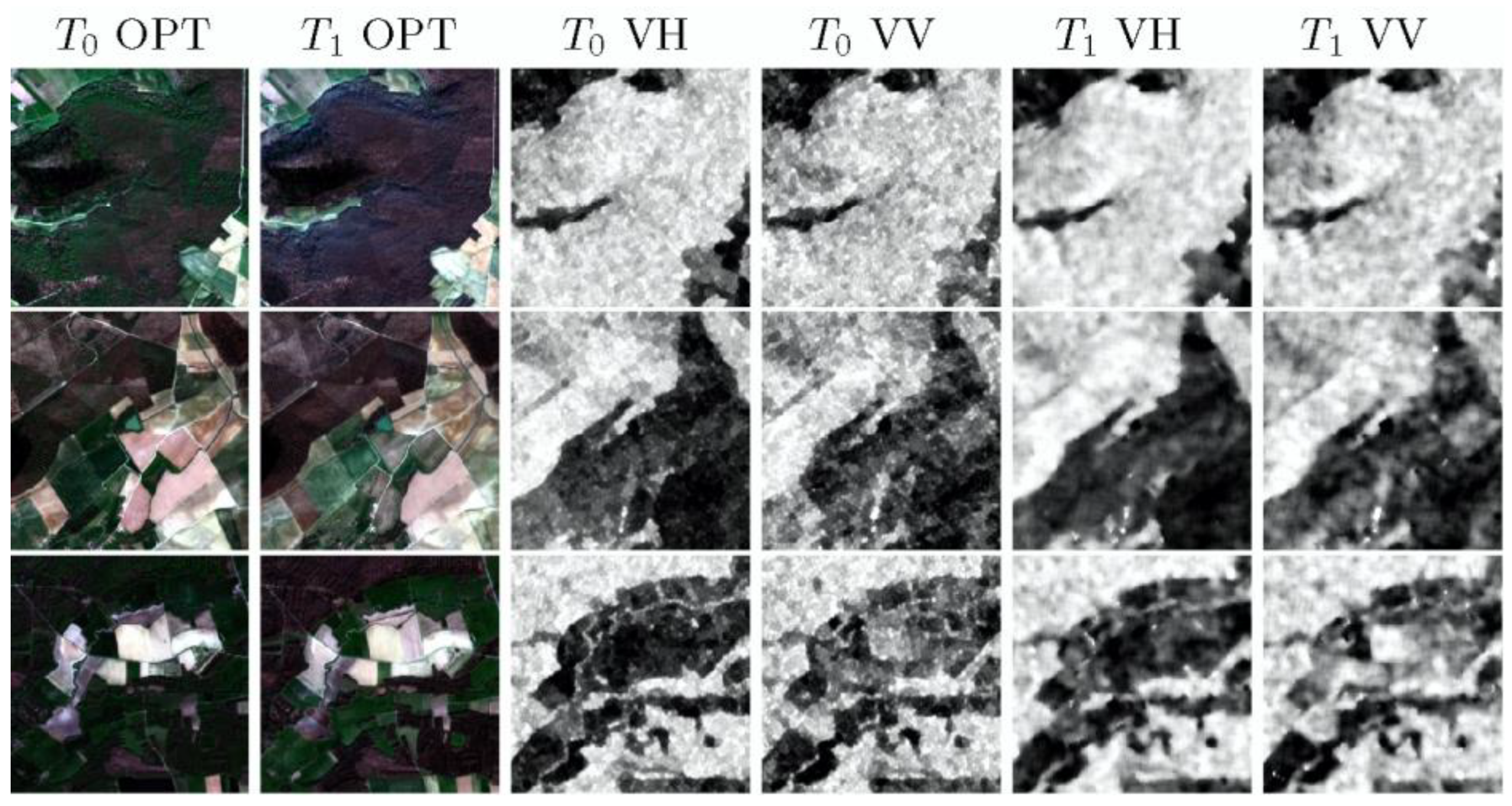
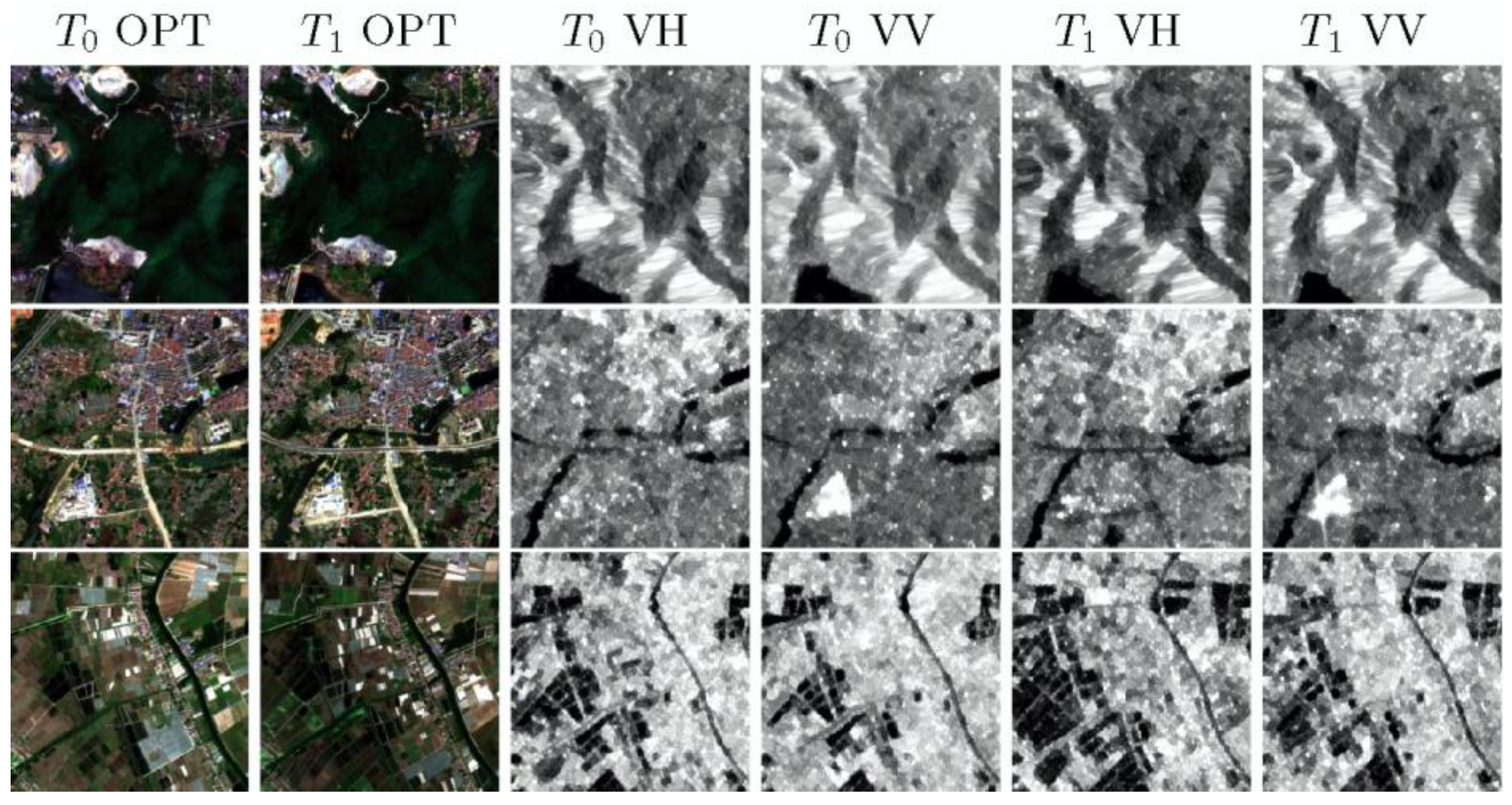
2. Dataset
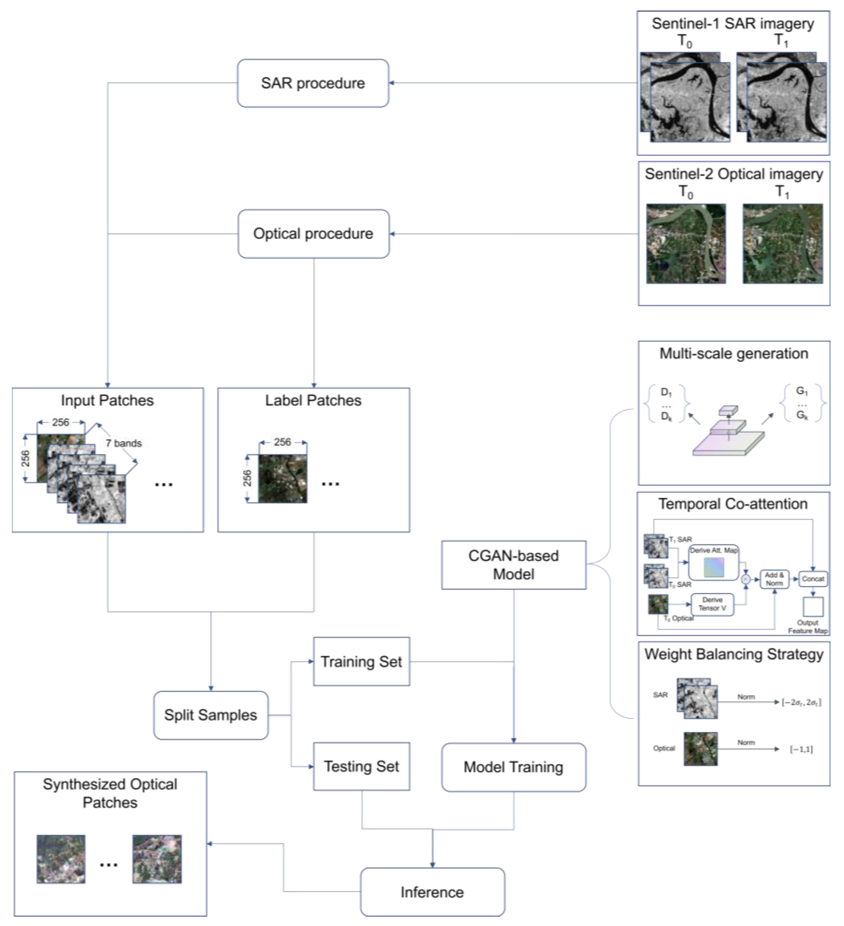
2.1. Dataset Procedure
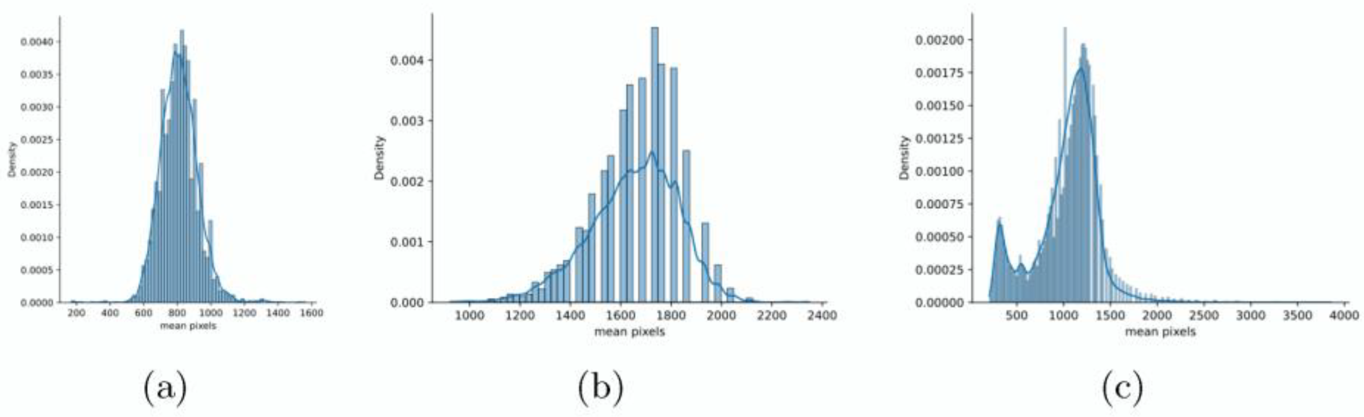
2.2. Special Features of the Dataset
3. Methodology
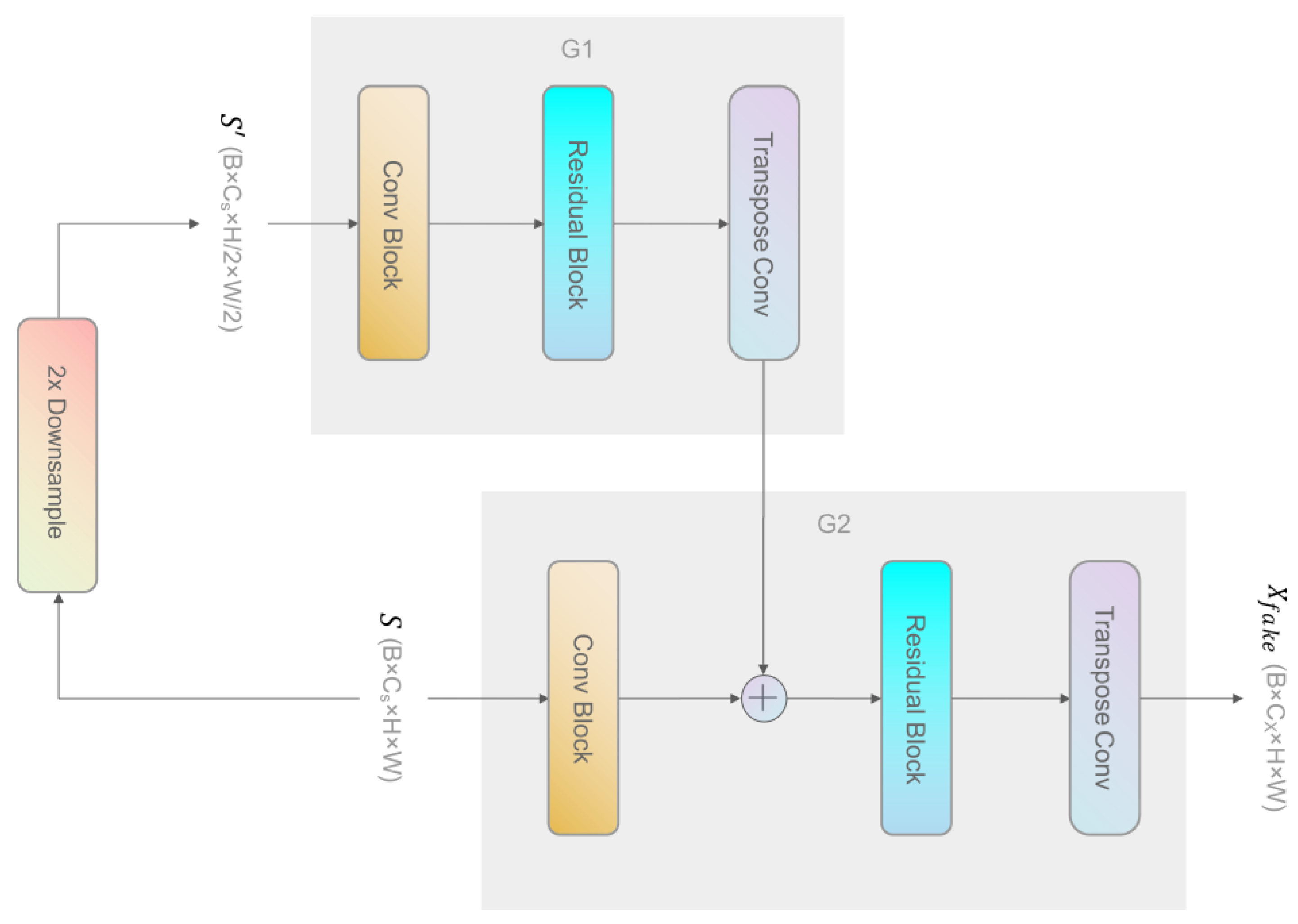
3.1. Coarse-to-Fine Generation
3.1.1. Multi-Scale Generation
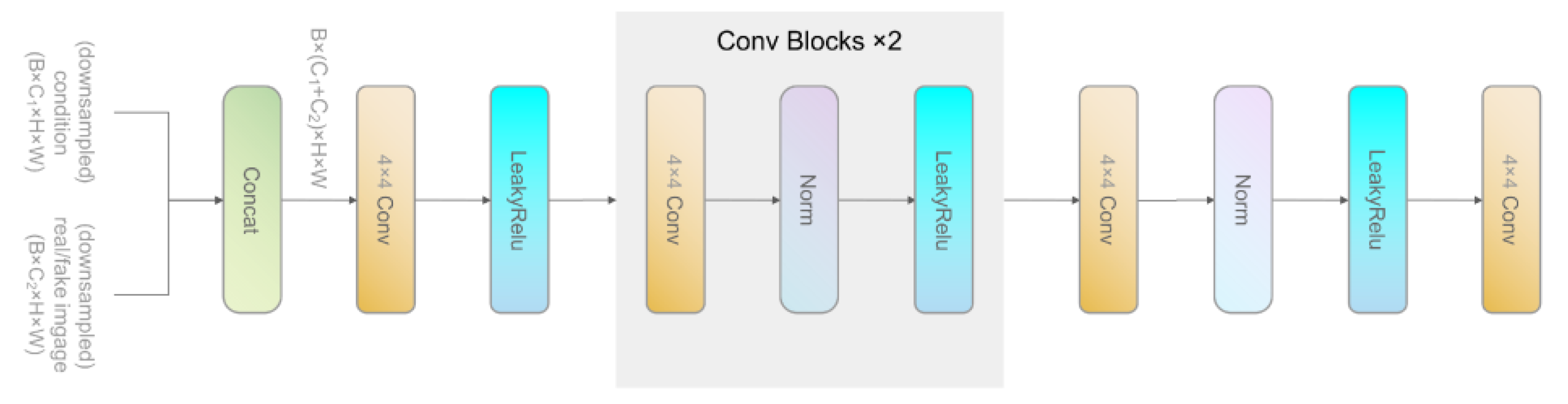
3.1.2. Multi-Scale Discrimination
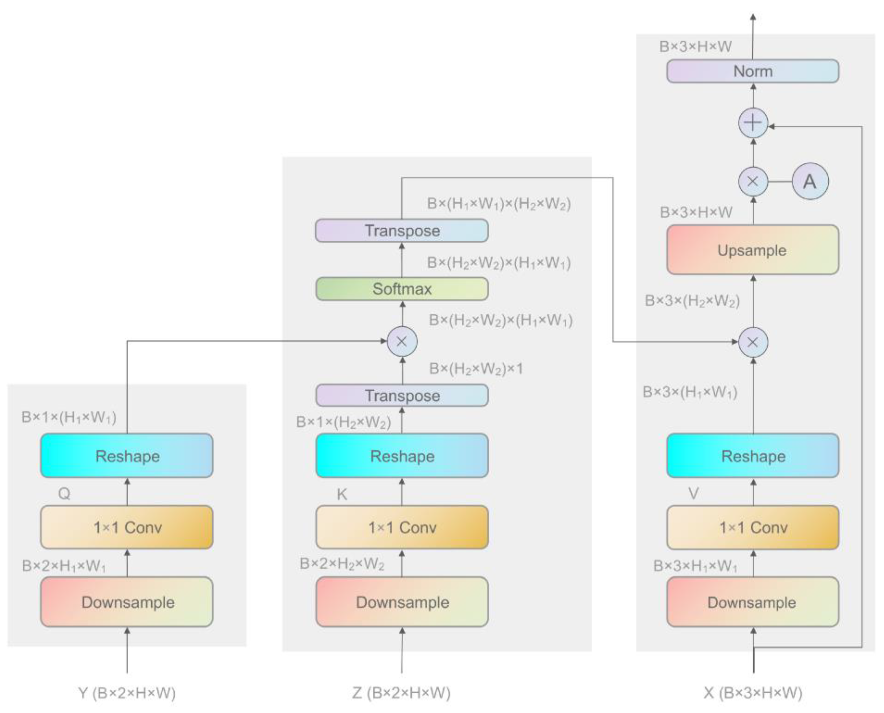
3.2. Temporal Co-Attention Guided Generator
3.3. Tackling Data Heterogeneity between Optical and SAR
4. Results and Discussion
4.1. Experiment Settings
4.2. Baseline
4.3. Evaluation Schemes and Metrics
- Fréchet Inception Distance (FID) [43]: It is a refinement of the inception score [44] and compares the mean and covariance of an Inception-v3 [45] network’s (pre-trained on ImageNet [46]) intermediate features for real and synthesized images. We employ FID for both datasets. Lower FID values mean closer distances between synthetic and real data distributions. The lower bound of FID is 0.
- Peak Signal to Noise Ratio (PSNR) [47]: This is a paired image quality assessment. It is a commonly used pixel-by-pixel measurement. Greater PSNR values indicate better quality.
- Structural Similarity Index Measures (SSIM) [48]: As another paired image quality assessment, the SSIM measurement is closer to human perception compared to PSNR [49] because it considers the inter-dependencies between pixels within a window of a specific size. We additionally adopt this metric as a measurement of the similarity between a synthesized image and the corresponding target image. To calculate the SSIM, we set the window’s size to 11. The upper bound of the SSIM is 1.0. A score closer to 1.0 indicates better quality.
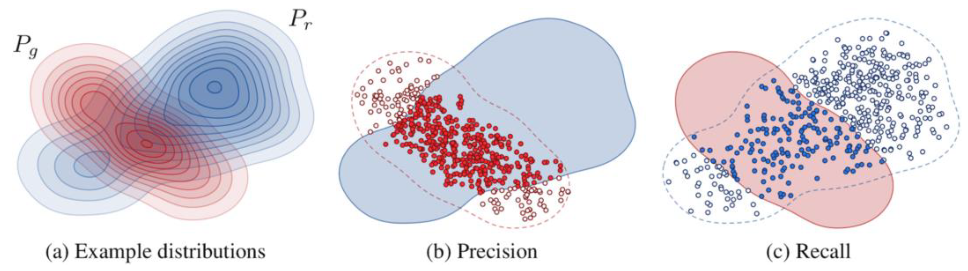
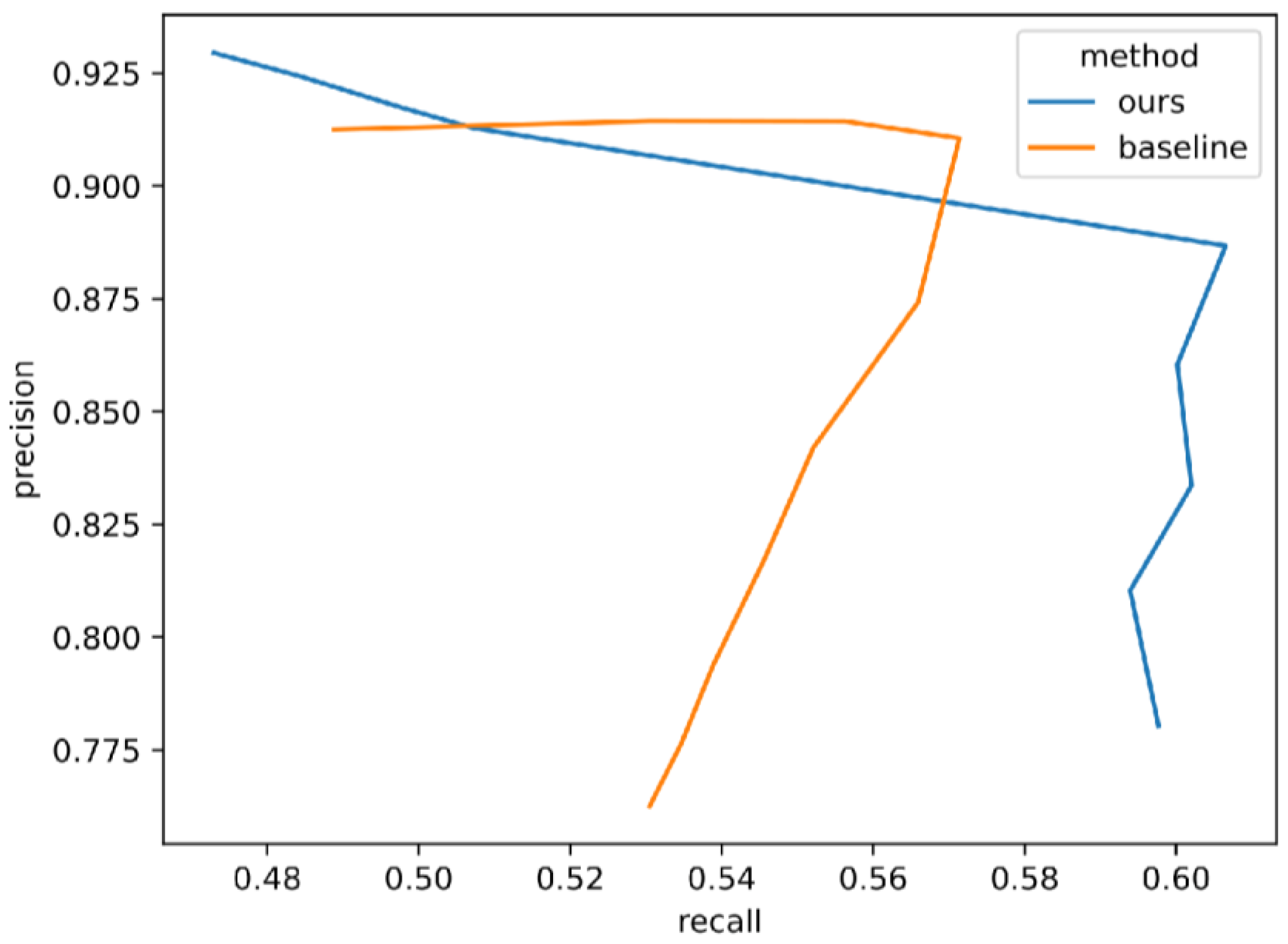
- Precision-Recall [50]: Precision and recall metrics are proposed as an alternative to FID when assessing the performance of GANs [50,51]. Precision quantifies the similarity of generated samples to the real ones, while recall denotes the capacity of a generator to produce all instances present in the set of real images (Figure 9). These metrics aim to explicitly quantify the trade-off between diversity (recall) and quality (precision).
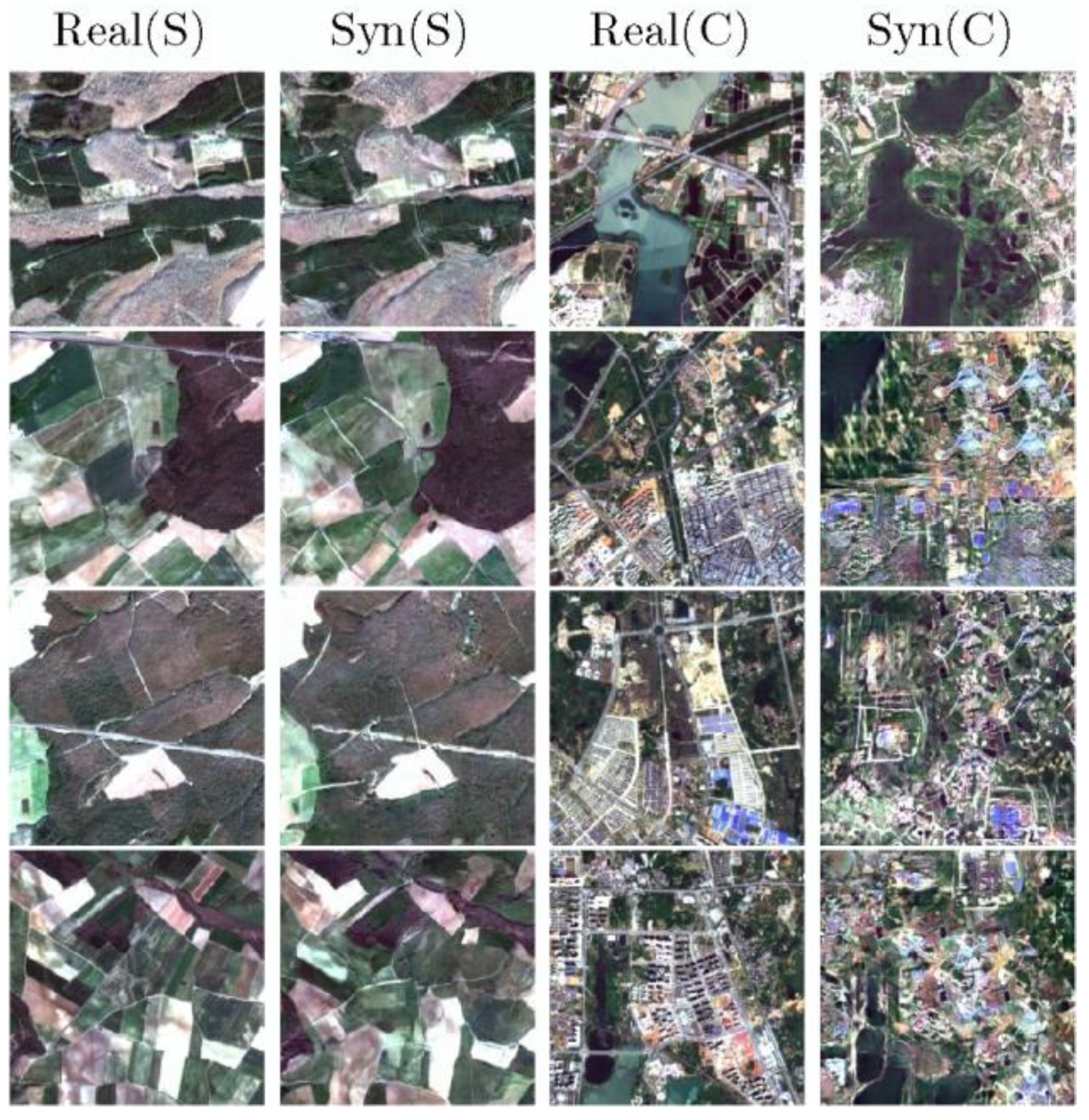
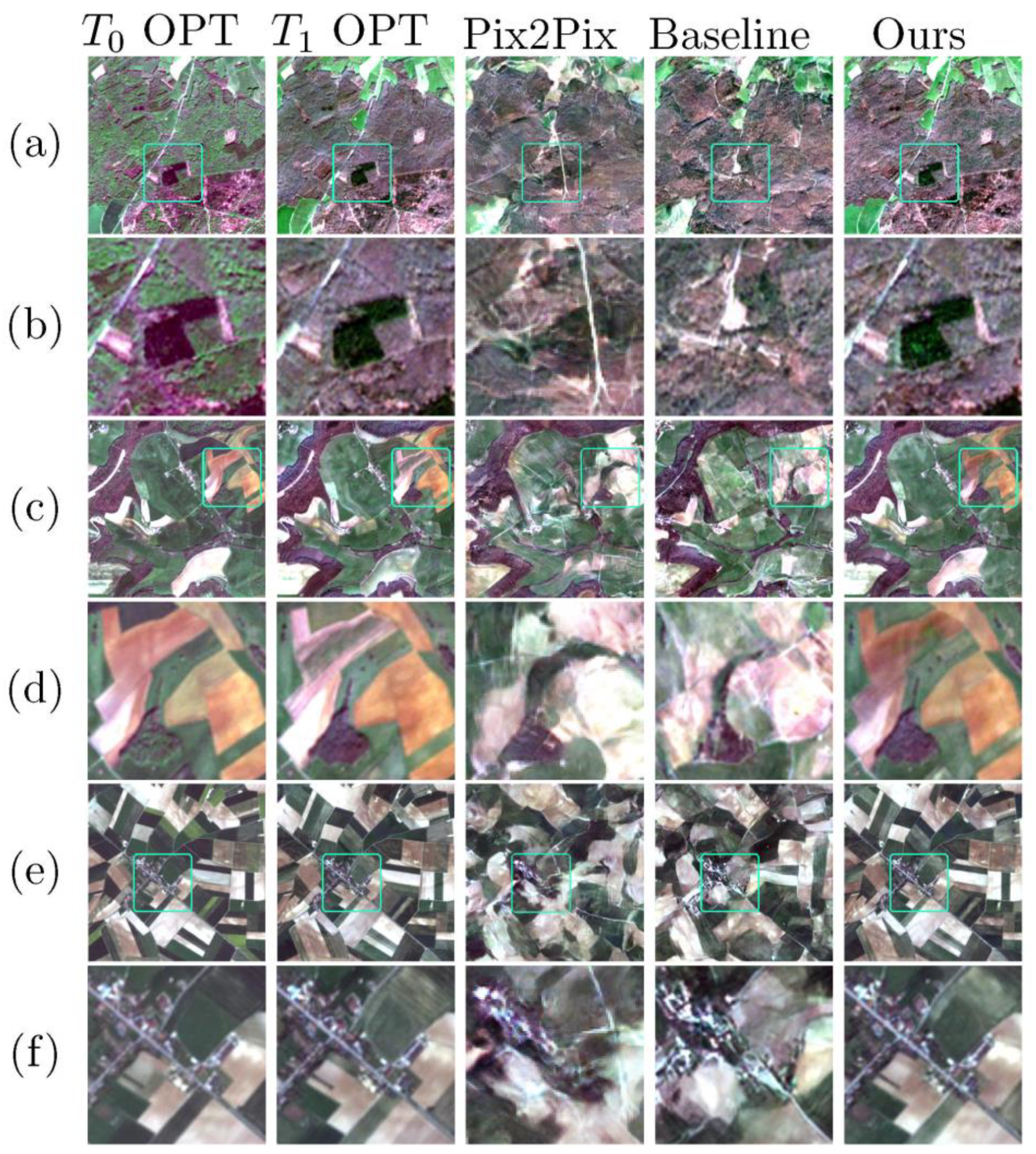
4.4. Comparisons of Simple Scenario Datasets
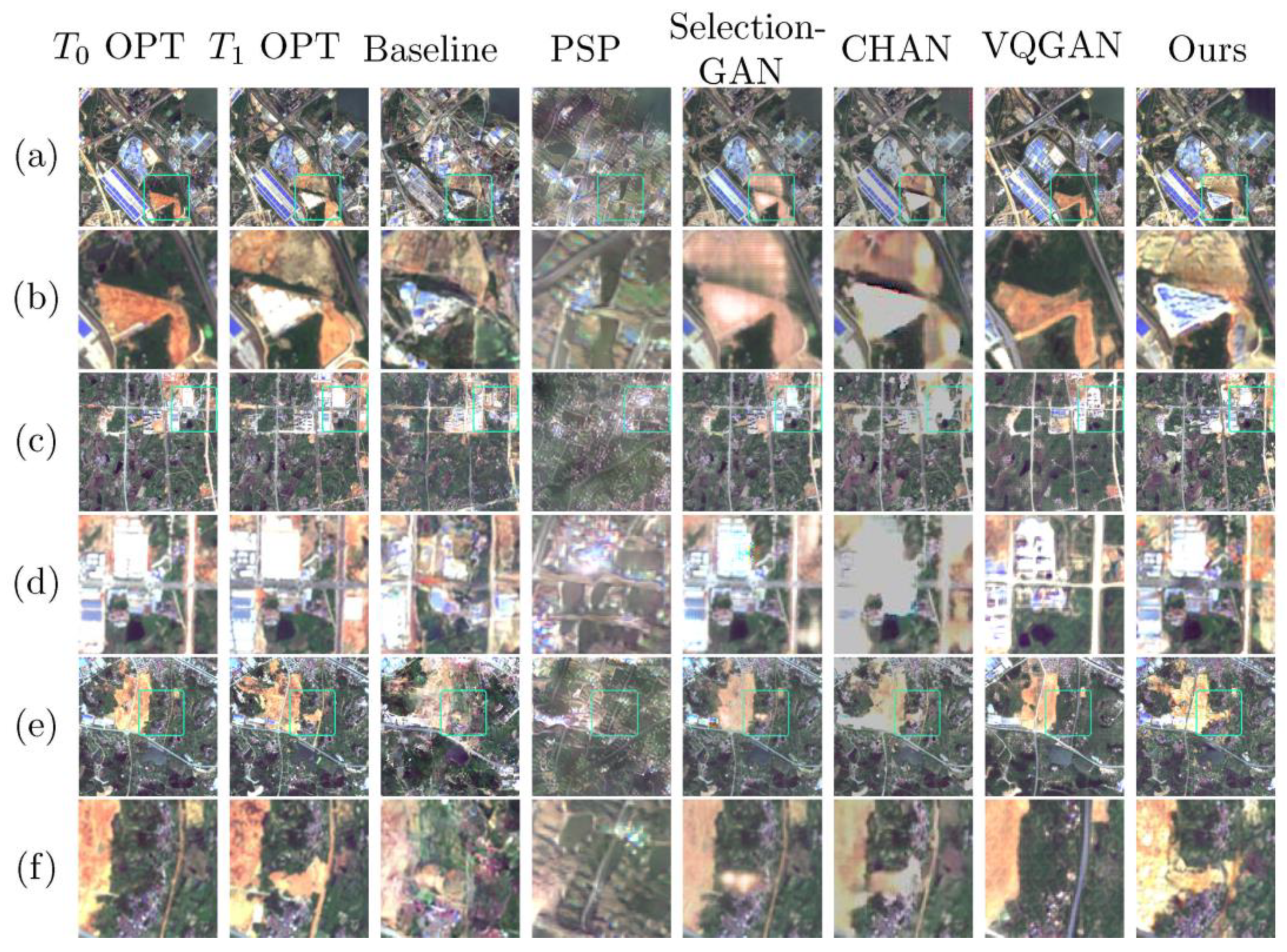
4.5. Comparisons of Complicated Scenario Datasets
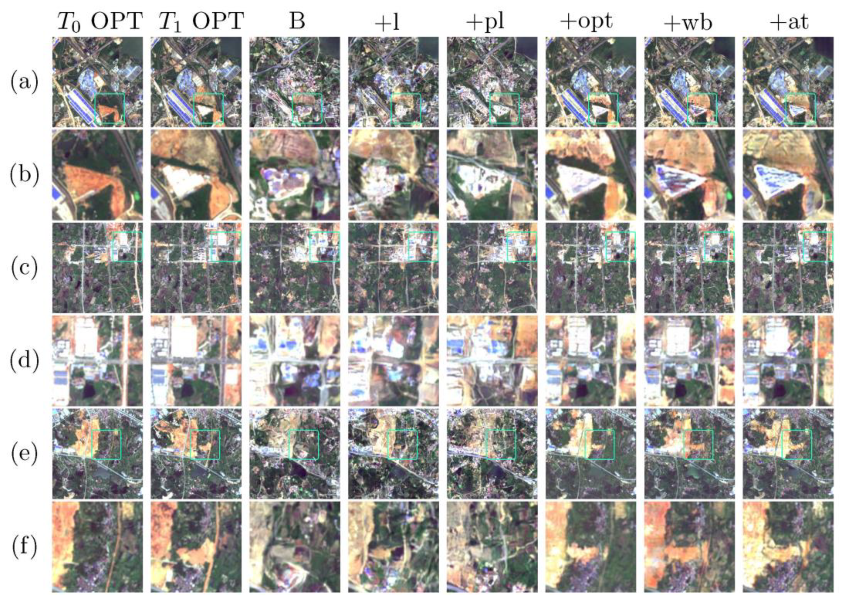
4.6. Ablation Study
5. Conclusions
Author Contributions
Funding
Data Availability Statement
Acknowledgments
Conflicts of Interest
Abbreviations
| GANs | Generative adversarial networks |
| CGAN | Conditional generative adversarial network |
| SAR | Synthetic aperture radar |
| I2I | Image-to-image |
| BOA | Bottom-of-Atmosphere |
| LSGANs | Least squares generative adversarial networks |
| PSNR | Peak signal-to-noise Ratio |
| SSIM | structural similarity index measure |
| FID | Fréchet Inception Distance |
| PR | precision-recall |
References
- Li, Z.; Shen, H.; Cheng, Q.; Li, W.; Zhang, L. Thick cloud removal in high-resolution satellite images using stepwise radiometric adjustment and residual correction. Remote Sens. 2019, 11, 1925. [Google Scholar] [CrossRef] [Green Version]
- Adrian, J.; Sagan, V.; Maimaitijiang, M. Sentinel sar-optical fusion for crop type mapping using deep learning and google earth engine. Isprs J. Photogramm. Remote Sens. 2021, 175, 215–235. [Google Scholar] [CrossRef]
- Huang, Z.; Dumitru, C.O.; Pan, Z.; Lei, B.; Datcu, M. Classification of large-scale high-resolution sar images with deep transfer learning. Ieee Geosci. Remote Sens. Lett. 2021, 18, 107–111. [Google Scholar] [CrossRef] [Green Version]
- Wang, L.; Yang, X.; Tan, H.; Bai, X.; Zhou, F. Few-shot class-incremental SAR target recognition based on hierarchical embedding and incremental evolutionary network. IEEE Trans. Geosci. Remote Sens. 2023, 61, 1–11. [Google Scholar] [CrossRef]
- Qin, J.; Liu, Z.; Ran, L.; Xie, R.; Tang, J.; Guo, Z. A target sar image expansion method based on conditional wasserstein deep convolutional GAN for automatic target recognition. IEEE J. Sel. Top. Appl. Earth Obs. Remote Sens. 2022, 15, 7153–7170. [Google Scholar] [CrossRef]
- Li, X.; Du, Z.; Huang, Y.; Tan, Z. A deep translation (gan) based change detection network for optical and sar remote sensing images. Isprs J. Photogramm. Remote Sens. 2021, 179, 14–34. [Google Scholar] [CrossRef]
- Saha, S.; Bovolo, F.; Bruzzone, L. Building change detection in VHR SAR images via unsupervised deep transcoding. IEEE Transactions on Geoscience and Remote Sensing 2021, 59, 1917–1929. [Google Scholar] [CrossRef]
- Fuentes Reyes, M.; Auer, S.; Merkle, N.; Henry, C.; Schmitt, M. Sar-to-optical image translation based on conditional generative adversarial networks—Optimization, opportunities and limits. Remote. Sens. 2019, 11, 2067. [Google Scholar] [CrossRef] [Green Version]
- Zhao, Y.; Celik, T.; Liu, N.; Li, H.-C. A comparative analysis of ganbased methods for sar-to-optical image translation. EEE Geosci. Remote. Sens. Lett. 2022, 19, 1–5. [Google Scholar] [CrossRef]
- Isola, P.; Zhu, J.-Y.; Zhou, T.; Efros, A.A. Image-to-image translation with conditional adversarial networks. In Proceedings of the IEEE Conference on Computer Vision and Pattern Recognition, Honolulu, HI, USA, 21–26 July 2017; pp. 1125–1134. [Google Scholar] [CrossRef] [Green Version]
- Bermudez, J.; Happ, P.; Oliveira, D.; Feitosa, R. SAR to optical image synthesis for cloud removal with generative adversarial networks. ISPRS Ann. Photogramm. Remote. Sens. Spat. Inf. Sci. 2018, IV-1, 5–11. [Google Scholar] [CrossRef] [Green Version]
- Grohnfeldt, C.; Schmitt, M.; Zhu, X. A conditional generative adversarial network to fuse SAR and multispectral optical data for cloud removal from sentinel-2 images. In Proceedings of the IGARSS 2018-2018 IEEE International Geoscience and Remote Sensing Symposium, Valencia, Spain, 22–27 July 2018; pp. 1726–1729. [Google Scholar] [CrossRef] [Green Version]
- Ebel, P.; Schmitt, M.; Zhu, X.X. Cloud removal in unpaired Sentinel-2 imagery using cycle-consistent GAN and SAR-optical data fusion. In Proceedings of the IGARSS 2020-2020 IEEE International Geoscience and Remote Sensing Symposium, Waikoloa, HI, USA, 26 September–2 October 2020; pp. 2065–2068. [Google Scholar] [CrossRef]
- Gao, J.; Yuan, Q.; Li, J.; Zhang, H.; Su, X. Cloud removal with fusion of high resolution optical and sar images using generative adversarial networks. Remote. Sens. 2020, 12, 191. [Google Scholar] [CrossRef] [Green Version]
- Zuo, Z.; Li, Y. A SAR-to-optical image translation method based on, PIX2PIX. In Proceedings of the 2021 IEEE International Geoscience and Remote Sensing Symposium IGARSS, Brussels, Belgium, 11–16 July 2021; pp. 3026–3029. [Google Scholar] [CrossRef]
- Lei, W. Polarimetric SAR Image Information Representation and Classification Based on Deep Learning. Ph.D. Thesis, Wuhan University, Wuhan, China, 2020. [Google Scholar] [CrossRef]
- Baier, G.; Deschemps, A.; Schmitt, M.; Yokoya, N. Synthesizing optical and SAR imagery from land cover maps and auxiliary raster data. IEEE Trans. Geosci. Remote. Sens. 2021, 60, 1–12. [Google Scholar] [CrossRef]
- Yang, X.; Wang, Z.; Zhao, J.; Yang, D. FG-GAN: A fine-grained generative adversarial network for unsupervised SAR-to-optical image translation. IEEE Trans. Geosci. Remote. Sens. 2022, 60, 1–11. [Google Scholar] [CrossRef]
- Mao, X.; Li, Q.; Xie, H.; Lau, R.Y.K.; Wang, Z.; Smolley, S.P. On the effectiveness of least squares generative adversarial networks. IEEE Trans. Pattern Anal. Mach. Intell. 2018, 41, 2947–2960. [Google Scholar] [CrossRef] [Green Version]
- Arjovsky, M.; Chintala, S.; Bottou, L. Wasserstein generative adversarial networks. In Proceedings of the International Conference on Machine Learning, Sydney, Australia, 6–11 August 2017; pp. 214–223. [Google Scholar]
- Karras, T.; Laine, S.; Aila, T. A style-based generator architecture for generative adversarial networks. EEE Trans. Pattern Anal. Mach. Intell. 2020, 43, 4217–4228. [Google Scholar] [CrossRef] [PubMed] [Green Version]
- Richardson, E.; Alaluf, Y.; Patashnik, O.; Nitzan, Y.; Azar, Y.; Shapiro, S.; Cohen-Or, D. Encoding in style: A stylegan encoder for image-to-image translation. In Proceedings of the IEEE/CVF Conference on Computer Vision and Pattern Recognition, Nashville, TN, USA, 20–25 June 2021; pp. 2287–2296. [Google Scholar] [CrossRef]
- Wang, T.-C.; Liu, M.-Y.; Zhu, J.-Y.; Tao, A.; Kautz, J.; Catanzaro, B. High-resolution image synthesis and semantic manipulation with conditional GANs. In Proceedings of the IEEE Conference on Computer Vision and Pattern Recognition, Salt Lake City, UT, USA, 18–23 June 2018; pp. 8798–8807. [Google Scholar] [CrossRef] [Green Version]
- Zhang, H.; Goodfellow, I.; Metaxas, D.; Odena, A. Self-attention generative adversarial networks. In Proceedings of the International Conference on Machine Learning, Long Beach, CA, USA, 6–15 June 2019; pp. 7354–7363. [Google Scholar]
- Gao, F.; Xu, X.; Yu, J.; Shang, M.; Li, X.; Tao, D. Complementary, heterogeneous and adversarial networks for image-to-image translation. IEEE Trans. Image Process. 2021, 30, 3487–3498. [Google Scholar] [CrossRef]
- Tang, H.; Xu, D.; Sebe, N.; Wang, Y.; Corso, J.J.; Yan, Y. Multi-channel attention selection GAN with cascaded semantic guidance for cross-view image translation. In Proceedings of the IEEE/CVF Conference on Computer Vision and Pattern Recognition, Long Beach, CA, USA, 15–20 June 2019; pp. 2417–2426. [Google Scholar] [CrossRef] [Green Version]
- Schmitt, M.; Hughes, L.H.; Zhu, X.X. The sen1-2 dataset for deep learning in SAR-optical data fusion. ISPRS Ann. Photogramm. Remote Sens. Spat. Inf. Sci. 2018, IV-1, 141–146. [Google Scholar] [CrossRef] [Green Version]
- Uziel, R.; Ronen, M.; Freifeld, O. Bayesian adaptive superpixel segmentation. In Proceedings of the IEEE/CVF International Conference on Computer Vision, Seoul, Republic of Korea, 27 October–2 November 2019; pp. 8469–8478. [Google Scholar] [CrossRef]
- Noa Turnes, J.; Castro, J.D.B.; Torres, D.L.; Vega, P.J.S.; Feitosa, R.Q.; Happ, P.N. Atrous cGAN for SAR to optical image translation. IEEE Geosci. Remote. Sens. Lett. 2020, 19, 1–5. [Google Scholar] [CrossRef]
- Zhang, H.; Xu, T.; Li, H.; Zhang, S.; Wang, X.; Huang, X.; Metaxas, D.N. StackGAN++: Realistic image synthesis with stacked generative adversarial networks. IEEE Trans. Pattern Anal. Mach. Intell. 2018, 41, 1947–1962. [Google Scholar] [CrossRef] [Green Version]
- Zhang, Z.; Xie, Y.; Yang, L. Photographic text-to-image synthesis with a hierarchically-nested adversarial network. In Proceedings of the IEEE Conference on Computer Vision and Pattern Recognition, Salt Lake City, UT, USA, 18–23 June 2018; pp. 6199–6208. [Google Scholar] [CrossRef] [Green Version]
- Jiang, L.; Zhang, C.; Huang, M.; Liu, C.; Shi, J.; Loy, C.C. Tsit: A simple and versatile framework for image-to-image translation. In Proceedings of the European Conference on Computer Vision, Glasgow, UK, 23–28 August 2020; pp. 206–222. [Google Scholar] [CrossRef]
- Esser, P.; Rombach, R.; Blattmann, A.; Ommer, B. ImageBART: Bidirectional context with multinomial diffusion for autoregressive image synthesis. Adv. Neural Inf. Process. Syst. 2021, 34, 3518–3532. [Google Scholar]
- Ho, J.; Saharia, C.; Chan, W.; Fleet, D.J.; Norouzi, M.; Salimans, T. Cascaded diffusion models for high fidelity image generation. J. Mach. Learn. Res. 2022, 23, 1–33. [Google Scholar]
- Wang, T.; Wu, L.; Sun, C. A coarse-to-fine approach for dynamic-to-static image translation. Pattern Recognit. 2022, 123, 108373. [Google Scholar] [CrossRef]
- Agustsson, E.; Tschannen, M.; Mentzer, F.; Timofte, R.; Gool, L.V. Generative adversarial networks for extreme learned image compression. In Proceedings of the IEEE/CVF International Conference on Computer Vision, Seoul, Republic of Korea, 27 October–2 November 2019; pp. 221–231. [Google Scholar] [CrossRef] [Green Version]
- Chen, C.; Gong, D.; Wang, H.; Li, Z.; Wong, K.-Y.K. Learning spatial attention for face super-resolution. IEEE Trans. Image Process. 2020, 30, 1219–1231. [Google Scholar] [CrossRef]
- Johnson, J.; Alahi, A.; Fei-Fei, L. Perceptual losses for real-time style transfer and super-resolution. In Computer Vision—ECCV 2016; Leibe, B., Matas, J., Sebe, N., Welling, M., Eds.; Springer: Cham, Switzerland, 2016; pp. 694–711. [Google Scholar] [CrossRef] [Green Version]
- Bermudez, J.D.; Happ, P.N.; Feitosa, R.Q.; Oliveira, D.A.B. Synthesis of multispectral optical images from SAR/optical multitemporal data using conditional generative adversarial networks. IEEE Geosci. Remote. Sens. Lett. 2019, 16, 1220–1224. [Google Scholar] [CrossRef]
- Louis, J. To Be Updated Sentinel 2 MSI—Level 2A Product Definition. Issue 4.4. 2016. Available online: https://sentinel.esa.int/documents/247904/1848117/Sentinel-2-Level-2A-Product-Definition-Document.pdf (accessed on 21 September 2022).
- Paszke, A.; Gross, S.; Massa, F.; Lerer, A.; Bradbury, J.; Chanan, G.; Killeen, T.; Lin, Z.; Gimelshein, N.; Antiga, L.; et al. PyTorch: An Imperative Style, High-Performance Deep Learning Library. arXiv 2019, arXiv:1912.01703. [Google Scholar] [CrossRef]
- Kingma, D.P.; Ba, J. Adam: A method for stochastic optimization. arXiv 2014, arXiv:1412.6980. [Google Scholar] [CrossRef]
- Heusel, M.; Ramsauer, H.; Unterthiner, T.; Nessler, B.; Hochreiter, S. GANs trained by a two time-scale update rule converge to a local nash equilibrium. Adv. Neural Inf. Process. Syst. 2017, 30, 6626–6637. [Google Scholar]
- Salimans, T.; Goodfellow, I.; Zaremba, W.; Cheung, V.; Radford, A.; Chen, X. Improved techniques for training GANs. Adv. Neural Inf. Process. Syst. 2016, 29, 2234–2242. [Google Scholar]
- Szegedy, C.; Vanhoucke, V.; Ioffe, S.; Shlens, J.; Wojna, Z. Rethinking the inception architecture for computer vision. In Proceedings of the IEEE Conference on Computer Vision and Pattern Recognition, Las Vegas, NV, USA, 27–30 June 2016; pp. 2818–2826. [Google Scholar] [CrossRef] [Green Version]
- Deng, J.; Dong, W.; Socher, R.; Li, L.-J.; Li, K.; Fei-Fei, L. Imagenet: A large-scale hierarchical image database. In Proceedings of the 2009 IEEE Conference on Computer Vision and Pattern Recognition, Miami, FL, USA, 20–25 June 2009; pp. 248–255. [Google Scholar] [CrossRef] [Green Version]
- Yuanji, W.; Jianhua, L.; Yi, L.; Yao, F.; Qinzhong, J. Image quality evaluation based on image weighted separating block peak signal to noise ratio. In Proceedings of the 2003 International Conference on Neural Networks and Signal Processing, Nanjing, China, 14–17 December 2003; Volume 2, pp. 994–997. [Google Scholar] [CrossRef]
- Wang, Z.; Bovik, A.C.; Sheikh, H.R.; Simoncelli, E.P. Image quality assessment: From error visibility to structural similarity. IEEE Trans. Image Process. 2004, 13, 600–612. [Google Scholar] [CrossRef] [Green Version]
- Sara, U.; Akter, M.; Uddin, M.S. Image quality assessment through FSIM, SSIM, MSE and PSNR—A comparative study. J. Comput. Commun. 2019, 7, 8–18. [Google Scholar] [CrossRef] [Green Version]
- Kynkäänniemi, T.; Karras, T.; Laine, S.; Lehtinen, J.; Aila, T. Improved precision and recall metric for assessing generative models. arXiv 2019, arXiv:1904.06991. [Google Scholar] [CrossRef]
- Sajjadi, M.S.M.; Bachem, O.; Lucic, M.; Bousquet, O.; Gelly, S. Assessing Generative Models via Precision and Recall. arXiv 2018, arXiv:1806.00035. [Google Scholar] [CrossRef]
- Esser, P.; Rombach, R.; Ommer, B. Taming transformers for high-resolution image synthesis. In Proceedings of the IEEE/CVF Conference on Computer Vision and Pattern Recognition, Nashville, TN, USA, 20–25 June 2021; pp. 12868–12878. [Google Scholar] [CrossRef]


| Parameters | Values |
|---|---|
| Optimizer | Adam [42] |
| β1 | 0.9 |
| β2 | 0.999 |
| Learning Rate | 2 × 10⁻⁴ |
| λ (Equation (5)) | 10 |
| Training Batch Size | 2 |
| Testing Batch Size | 1 |
| Metrics | Pix2Pix | Baseline | Ours |
|---|---|---|---|
| FID ↓ | 221.1 | 99.9 | 69.46 |
| PSNR ↑ | 13.80 | 18.36 | 21.89 |
| SSIM ↑ | 0.23 | 0.62 | 0.78 |
| Metrics | Baseline | PSP | Selection-GAN | CHAN | VQGAN Transformer | Ours |
|---|---|---|---|---|---|---|
| FID ↓ | 121.35 | 148.10 | 82.02 | 112.36 | 108.14 | 80.60 |
| PSNR ↑ | 12.14 | 14.0 | 18.53 | 17.55 | 13.63 | 20.79 |
| SSIM ↑ | 0.17 | 0.19 | 0.66 | 0.60 | 0.25 | 0.62 |
| Metrics | B | B + l | B + l + pl | B + l + pl + opt | B + l + pl + opt + wb | B + l+pl + opt + wb + at |
|---|---|---|---|---|---|---|
| FID ↓ | 149.03 | 133.80 | 108.25 | 84.43 | 83.53 | 80.60 |
| (−10.22%) * | (−27.36%) | (−43.35%) | (−43.95%) | (−45.92%) | ||
| PSNR ↑ | 11.97 | 12.34 | 13.33 | 16.45 | 17.96 | 20.79 |
| (+3.09%) | (+11.36%) | (+37.43%) | (+50.04%) | (+73.68%) | ||
| SSIM ↑ | 0.17 | 0.18 | 0.21 | 0.58 | 0.57 | 0.62 |
| (+5.88%) | (+23.53%) | (+241.18%) | (+235.29%) | (+264.71%) |
Disclaimer/Publisher’s Note: The statements, opinions and data contained in all publications are solely those of the individual author(s) and contributor(s) and not of MDPI and/or the editor(s). MDPI and/or the editor(s) disclaim responsibility for any injury to people or property resulting from any ideas, methods, instructions or products referred to in the content. |
© 2023 by the authors. Licensee MDPI, Basel, Switzerland. This article is an open access article distributed under the terms and conditions of the Creative Commons Attribution (CC BY) license (https://creativecommons.org/licenses/by/4.0/).
Share and Cite
Weng, Y.; Ma, Y.; Chen, F.; Shang, E.; Yao, W.; Zhang, S.; Yang, J.; Liu, J. Temporal Co-Attention Guided Conditional Generative Adversarial Network for Optical Image Synthesis. Remote Sens. 2023, 15, 1863. https://doi.org/10.3390/rs15071863
Weng Y, Ma Y, Chen F, Shang E, Yao W, Zhang S, Yang J, Liu J. Temporal Co-Attention Guided Conditional Generative Adversarial Network for Optical Image Synthesis. Remote Sensing. 2023; 15(7):1863. https://doi.org/10.3390/rs15071863
Chicago/Turabian StyleWeng, Yongchun, Yong Ma, Fu Chen, Erping Shang, Wutao Yao, Shuyan Zhang, Jin Yang, and Jianbo Liu. 2023. "Temporal Co-Attention Guided Conditional Generative Adversarial Network for Optical Image Synthesis" Remote Sensing 15, no. 7: 1863. https://doi.org/10.3390/rs15071863