Spatial Visualization Based on Geodata Fusion Using an Autonomous Unmanned Vessel

Abstract

The visualization of riverbeds and surface facilities on the banks is crucial for systems that analyze conditions, safety, and changes in this environment. Hence, in this paper, we propose collecting, and processing data from a variety of sensors—sonar, LiDAR, multibeam echosounder (MBES), and camera—to create a visualization for further analysis. For this purpose, we took measurements from sensors installed on an autonomous, unmanned hydrographic vessel, and then proposed a data fusion mechanism, to create a visualization using modules under and above the water. A fusion contains key-point analysis on classic images and sonars, augmentation/reduction of point clouds, fitting data and mesh creation. Then, we also propose an analysis module that can be used to compare and extract information from created visualizations. The analysis module is based on artificial intelligence tools for the classification tasks, which helps in further comparison to archival data. Such a model was tested using various techniques to achieve the fastest and most accurate visualizations possible in simulation and real case studies.

1. Introduction

The shore is an important area that changes dynamically. The upper part comprises the shore and the natural land cover, which can be distinguished from objects built and permanently modified by man: quays, docks, flood banks, dams, bridges, piers, locks, and marinas. The underwater part comprises the shape of the bottom with all objects located on it. Quite often hydro-technical structures are located both above and below the water. Shoreal areas are often shallow, and their shape is important from the point of view of navigation safety and environmental protection. Currently, shoreal zone monitoring includes land and hydrographic measurements [1]. Several teams collect data using different devices or systems, process the data separately and then merge it into one whole. This is very time-consuming, which means that the cost of acquiring data or final maps from this zone is high.

Today, it is possible to amass a huge amount of spatial information in a relatively short time. The problem is how to visualize spatial data that have different characteristics from different sensors such that they are consistent and sufficiently accurate [2]. Because of the different sensor characteristics, it is not possible to adapt them directly, so it is necessary to develop new methods for vessels equipped with several sensors that collect information on and below the surface. Undertaking this task requires solving a few problems from geoinformatics, hydrography, navigation, data processing, mathematical modeling, and computer science [3]. The system we are building is a system related to geoinformatics because all spatial data is geographic data and subject to further analysis. Hydrography because we collect and process hydrographic data. The same applies to data processing. Navigation is used during spatial data collection. Computer science because we write the unique code ourselves in the free python language and informatics knowledge is needed for this. Mathematical modeling, on the other hand, is used during data fusion at many stages of our research.

Currently, the fusion of LiDAR, and camera data is widely used on autonomous vehicles, mainly to avoid collisions, although this Simultaneous Localization and Mapping method orients the vehicle in the surrounding terrain, its use on the water is still a subject of research. Large areas of the world’s shoreal marine environment remain poorly characterized because they have not been mapped with sufficient accuracy even though spatial data acquisition systems have a resolution high enough to meet a wide range of societal needs. Accelerating the pace of seafloor mapping requires the collection of very large datasets, but these primarily include data from a single sensor [4].

Systems that include information from a single sensor are relatively popular, but most are designed for a limited range of tasks. The analysis of geospatial data and their fusion has been discussed for many years [5,6]. One solution is to integrate LiDAR with MBES as presented in [7,8]. Another example is described in [9], where the authors show proposed algorithms for combining MBES and sonar for underwater data. The simultaneous use of sensors are also applicable to robot navigation (e.g., LiDAR and camera [10]) or in the bottom mapping by an autonomous underwater vehicle (AUV), which collects data to build 3D maps of underwater areas such as mapping the structure and appearance of coral reefs. The system is based on the fusion of data from a single camera and a multibeam echosounder [11]. Another example is the algorithms proposed by [12] but they only include data from LiDAR and the camera. In [13], the authors presented a combination of both types. Raster data were processed using graphical methods (e.g., sharpening), and vector data were selected to extract only specific points above a certain height. Then the image was segmented using both types of data. The integration processed the two images and exported the saturation of LiDAR points as an image. Common examples of combining are data mapping and reconstruction analysis [14]. In the research results, the authors focused on combining images with information about depths (obtained from 3D LiDAR data). The connection was based on the use of visual odometry and graphical optimization. The idea can be described as extracting video frames and point clouds located on the same measurement and then plotting them for further analysis. Again, in [15], the integration was based on processed data. The point cloud was adjusted to the appropriate image frames; points were selected concerning the OZ axis; and then, the cloud visualization was saved as a 2D flat image, which was used for segmentation analysis against raster data. Combining MBES and LiDAR data can also be used for seafloor classification based on feature extraction and classification [16].

The fusion of raster and vector data was also used to match the data resolution in [17]. The algorithm was based on the geometric alignment of the two data streams and then the resolution was matched. Another approach is to extract features from both data types and give a classification. The idea of extraction was based on processing vector data into a 2D image as shown by [18]. Another type of fusion was described by [19], which proposed using convolutional neural network (CNN) architecture. The LiDAR point cloud projection was also presented as a 2D image, and the CNN used the image data to segment a road. It is worth noting that the use of neural networks is associated with the preparation of large training sets. In the case of segmentation, two sets are prepared—the original data from the sensors and the expected results, i.e., initial segmentation. The fusion of image and numerical data also takes place by applying graphic images to the mesh, which in turn is understood as to applying a texture to the model as it was proposed by [20]. No solution integrated output data from four sensors: fusion of output data from four sensors is new in the global geoinformatics market. There was also no visualization of the integrated data in the form of a spherical projection of panoramic data, which would enable a complex analysis of the underwater, and surface situations. Except for the fusion, a very important task is the use of these solutions which can be applied mainly in the analysis, comparison and investigation of different objects and how there are changes with time [21,22]. Interesting approach is to create integrated mapping system [23], where the authors described analysis of modeled solution. A similar idea is to use mobile technology for mapping images [24]. This solution combine selected neural architecture with mobile mapping.

The main aim of the paper is to develop an innovative system for the purpose of presenting data from various sensors that can be used to analyze areas. The proposed methodology may enable quick analysis of this data and its visualization. As an example, this approach allows for an analysis of changes in the shape of a river bottom and the terrain in this zone is frequent. The data are collected simultaneously during one measurement path and then sent to a module that creates a spherical projection of panoramic data. Information from the MBES and sonar goes to the integrated underwater data module; whereas information from the LiDAR system and the camera is transferred to the integrated data module on the surface. Both modules form the integrated data module (data fusion), which sends information to the processing and visualization module. It consists of data fusion and visualization modules in the form of a spherical projection of panoramic data. The data fusion module, which is responsible for complex data integration, consists of the database and spherical data modules. In the final stage, the data fusion module sends the integrated information in the form of a numerical three-dimensional projection to the data visualization module. Its components are the geo composition module responsible for layers and map attributes, and the presentation module, which is related to symbolization and map perception.

This paper focuses on presenting the initial design concept, preliminary operating models and data fusion methods. The initial schemes were modeled and tested on the simulation task with different data gathered in the real environment. The main contributions of this paper are:

• model and schemes of the fusion of four different kinds of data to obtain a spherical projection of panoramic data,
• investigating the use of different algorithms including machine learning for data processing in geodata tasks,
• real case studies of the proposal by use of an autonomous unmanned vessel.

2. Method

In this section, we describe the proposed methodology and all its components. The section is split into the underwater data fusion model, the above data fusion model, a combination of previous results and an analysis module.

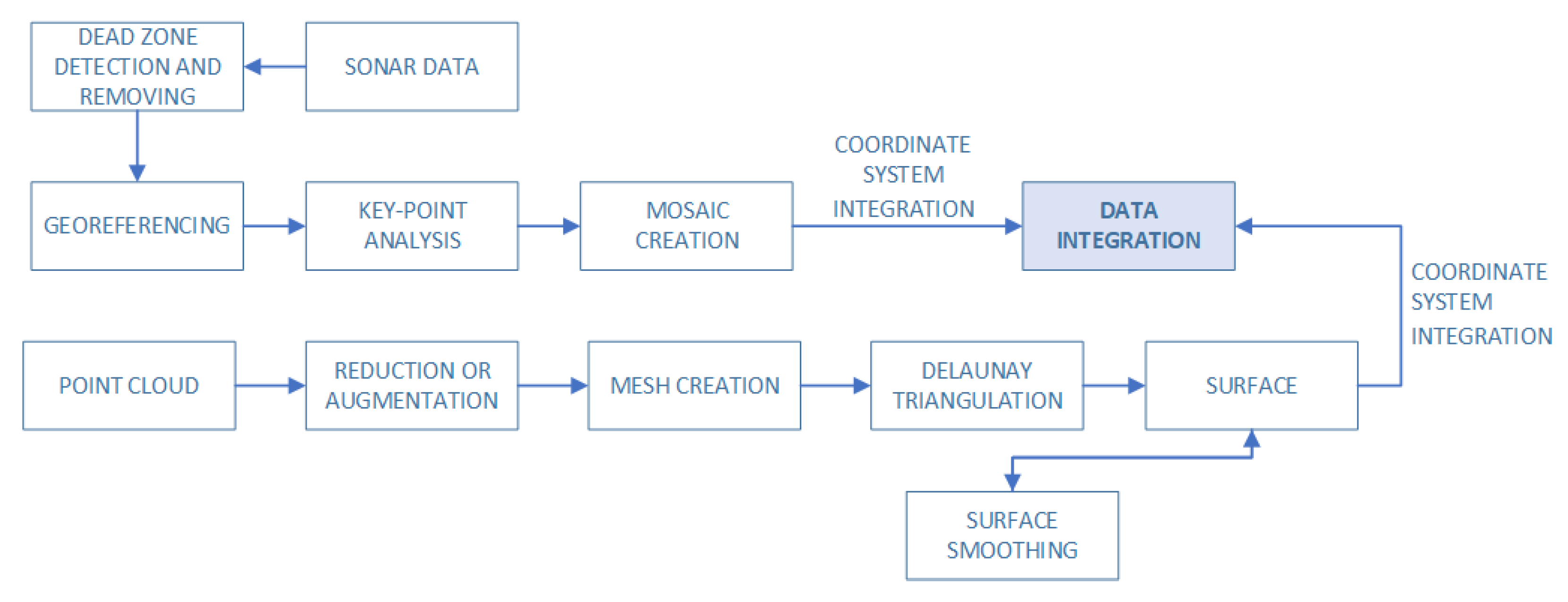
2.1. Underwater Data Fusion: Bathymetric Points and Sonar Data

This subsection describes the processing of bathymetric data and sonar images to create a merged underwater surface. The proposed approach is based on processing obtained data and its combination. It is done by analyzing the points clouds and their verification by a developed condition that can be interpreted as decision-making. Then, these points are used to create a surface that will get the sonar data as a georeference. A simplified step-by-step process as a schema as shown in Figure 1. Integration of underwater data is based on the combination of two selected data, i.e., a point cloud and signal reflection data obtained from sonar. The integration of these data is to enable merging by using sonar to obtain details on the surface designated with MBES data. Such integration allows merging selected types of data (placed in the database) to get the correct visualization and analysis capabilities.

2.1.1. Bathymetric Points

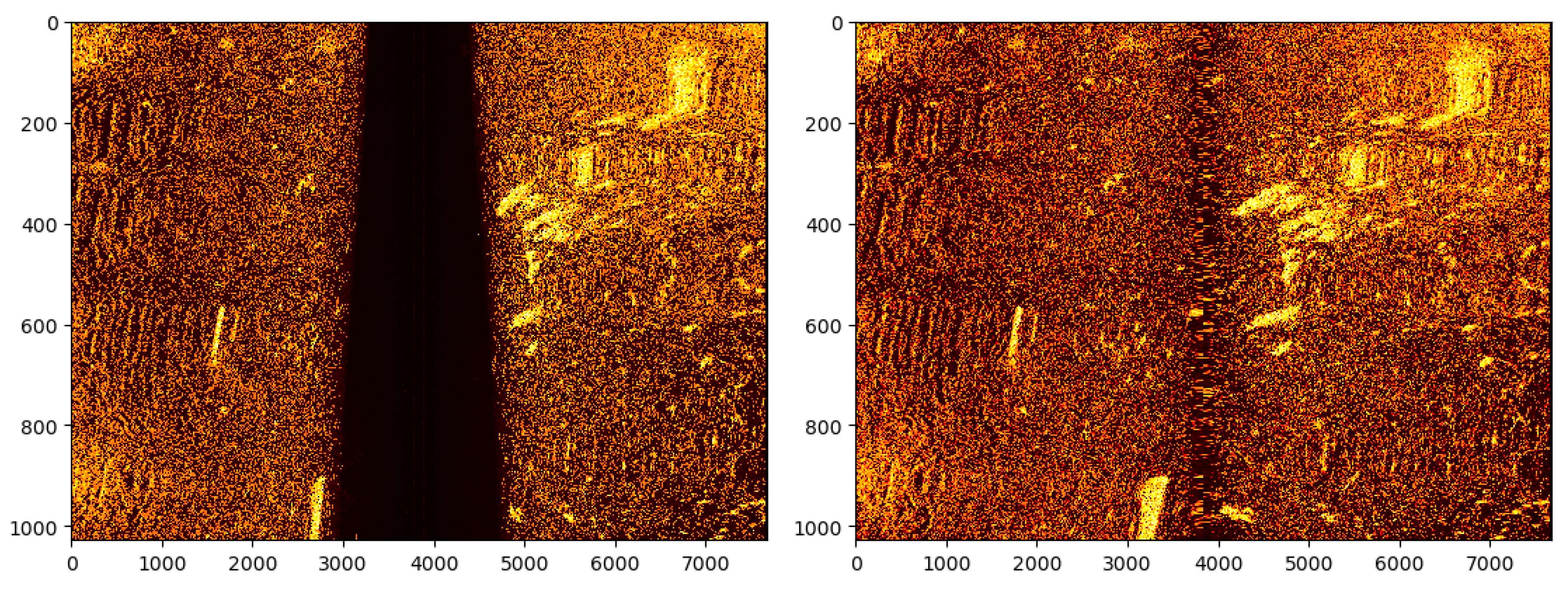
Point clouds from bathymetric data can be represented as a set of s points $\mathbf{B}=\{{\mathbf{p}}_{\mathbf{0}},{\mathbf{p}}_{\mathbf{1}},\dots ,{\mathbf{p}}_{\mathbf{s}-\mathbf{1}}\}$ where $\mathbf{p}=[x,y,z]$. In the case of a small number of points, an augmentation can be made. The usual way to create new points is by interpolation [25,26]. The idea is to find a new potential point between at least two others. In the opposite case, when there are too many points, and simulation is difficult then this number can be reduced by down-sampling [27]. It is worth paying attention to the chosen sampling method here because it is based on 2.5D which is called pseudo-3D, i.e., using the principle of isometric projection most often. When using 3D, we get a three-dimensional model. In the case of the sampling algorithm used, it works on the principle of using the selected coordinates to obtain the target. Graphics programs like Blender use 3D sampling while spatial data analysis software like ArcGIS uses 2.5D. During measurements, a recording or measuring error may occur, which will cause a certain point to be erroneous. A statistical approach can be used for these purposes. For example, the three-sigma rule can be used to determine outliers that can be removed before further processing.

In our proposition, we analyze the number of points set according to the average number of points in a given area. It is made by the calculation of the average number of points needed to cover the analyzed area. Used set $\mathbf{B}$ is spanned on the OX and OY axes, hence the maximum area covered by the points are: $\langle {min}_i\left(x_i\right),{max}_i\left(x_i\right)\rangle \times \langle {min}_i\left(y_i\right),{max}_i\left(y_i\right)\rangle$ (where $i\in \{0,1,\dots ,s-1\}$). This set can be split into $\kappa =({max}_i\left(x_i\right)-{min}_i\left(x_i\right))·({max}_i\left(y_i\right)-{min}_i\left(y_i\right))$ equals subareas. We evaluate the average number of existing points in a given set $\mathbf{B}$ on one unit of such subarea to decide if there is a need for an augmentation/down-sampling method. It can be done according to the following equation:

$$\left\{\begin{array}{c}{\displaystyle \mathrm{if}\exists \mathbf{b}\subset \mathbf{B},0.9·\left|\mathbf{b}\right|<\frac{\left|\mathbf{B}\right|}{\kappa },\mathrm{then}\mathrm{augmentation},}\hfill \\ {\displaystyle \mathrm{if}\exists \mathbf{b}\subset \mathbf{B},1.1·\left|\mathbf{b}\right|>\frac{\left|\mathbf{B}\right|}{\kappa },\mathrm{then}\mathrm{down}-\mathrm{sampling},}\hfill \\ \mathrm{in}\mathrm{other}\mathrm{cases},\mathrm{the}\mathrm{number}\mathrm{of}\mathrm{elements}\mathrm{in}\mathrm{the}\mathrm{set}\mathrm{is}\mathrm{on}\mathrm{average},\hfill \end{array}\right.$$

(1)

where $\mathbf{b}$ is a subset from $\mathbf{B}$ that describe mentioned above subarea. In the next step, all points are used to create a mesh by using the Delaunay triangulation method [28,29]. It works by determining if a given point is inside the circle described by the triangle. At first, a super triangle is created that contains all points. Then for a given point ${\mathbf{p}}_{\mathbf{i}}=[x_i,y_i,z_i]$ we check to see if it is in a circle described in a triangle composed of points ${\mathbf{p}}_{\mathbf{1}}$, ${\mathbf{p}}_{\mathbf{2}}$, ${\mathbf{p}}_{\mathbf{3}}$. It is evaluated by the following condition:

$$det\left[\begin{array}{cccc}{x}_1& y_1& x_1^2+y_1^2& 1\\ x_2& y_2& x_2^2+y_2^2& 1\\ x_3& y_3& x_3^2+y_3^2& 1\\ xi& y_i& x_i^2+y_i^2& 1\end{array}\right]>0.$$

(2)

In this way, a mesh composed of triangles based on a point cloud will be generated.

2.1.2. Sonar Data

In the case of sonar data, analysis of the seabed quite often ends with several sonar measurements, each of which is saved in a separate file, usually with the *.xtf extension. If these files are georeferenced, the data can be combined by overlaying maps with respect to their location in a specific coordinate system. However, it is not always possible to take advantage of georeferencing. Consequently, any file can be converted to a bottom image. Then, all images should be combined into one (hereinafter referred to as “texture”). It can be done by the use of known key-point algorithms like ORB [30], BRISK [31], AGAST [32], SIFT [33,34] or SURF [35]. These algorithms allow us to locate key points and adjust them in different images. The sonar images are combined into a so-called mosaic that can be used as a texture to represent the bottom. Despite obtaining the image, the issue of georeferencing remains.

Our sonar data processing proposal is based on the analysis of files obtained from the side-scan sonar. As a result, data are presented as a set of signal reflection values from the bottom or obstacle. Hence, sonar data contain data on the left and right sides of the Sonar. The space under it is the so-called dead zone that has not been examined. The first step in such an analysis is to generate an image based on the value of reflection signals from Sonar. Then, with the help of an edge detection algorithm, we detect the dead zone area, which is removed. The image on the left and right are sewn (but on the same dimension—see Figure 2). Having such an image, it remains only to make a georeferencing, which is possible by collecting the value of starting coordinates and the end of sonar measurements (these values are available as metadata in XTF files). The georeferencing is based on determining value $(x,y)$ for each pixel. This is performed by determining the values using the estimation of how far the sonar beam reaches, which allows you to determine two coordinates for a pixel in the middle and border. The coordinates of the points between are determined by dividing the distance between these points by the number of desired points. As a result, these points are equal to each other [36]. Mosaic can be based on applying images with a coordinate system. However, there are quite often deviations or problems in sonar measurement. Hence, we suggest the additional use of stitching algorithms based on key points analysis to match these images. Finally, the image was created by applying sonar images and their matching creates a sonar mosaic, which is exported to the geotiff file, containing the image and coordinates of these pixels.

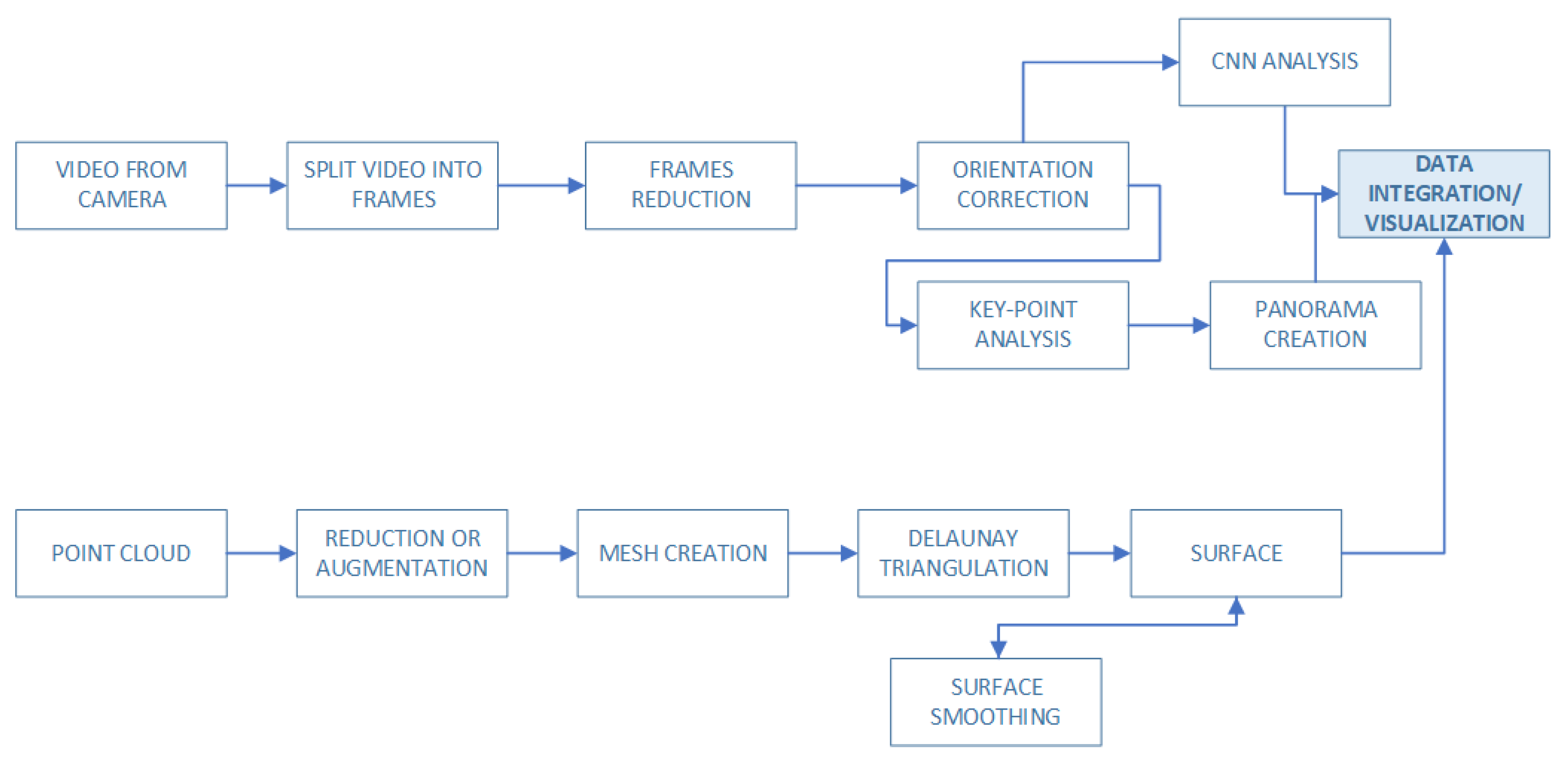
2.2. Above the Sea Data Fusion Model: Lidar and Camera Video

Above the sea, the area can be processed in a manner similarly to underwater data as described in Section 2.1. The LiDAR point can be processed to create a surface, and the video to create texture (or to use as colors for LiDAR points/mesh). However, the video file from the camera is composed of many frames: the classic camera operates at 24 frames per second, while the metric one operates at 2. Therefore, it is important to split the video file into a set of frames.

In the case of videos recorded with ordinary cameras, the number of frames to process is huge and not needed. Hence, we propose to analyze the frames at a constant time interval t (e.g., $t=1$ or $t=2$). The next problem is the shoreline on the frames. The recorded image will also contain a portion of the water surface that should not be analyzed. For this purpose, we propose to trim each frame in relation to the borderline. It can be done by using an image-processing filter (edge detection, reduction), and interpolation, or some segmentation by the u-net models [37] (both cases are discussed below). If the image becomes skewed about the shoreline trim, it should be rotated by simple image processing. Then each frame can be treated as an image and key-point analysis can merge all these images into one stitched view that can be added to the surface. The Proposed technique is based on a combination of different approaches like image processing, machine learning and cloud points analysis. A visualization of these steps is shown in Figure 3.

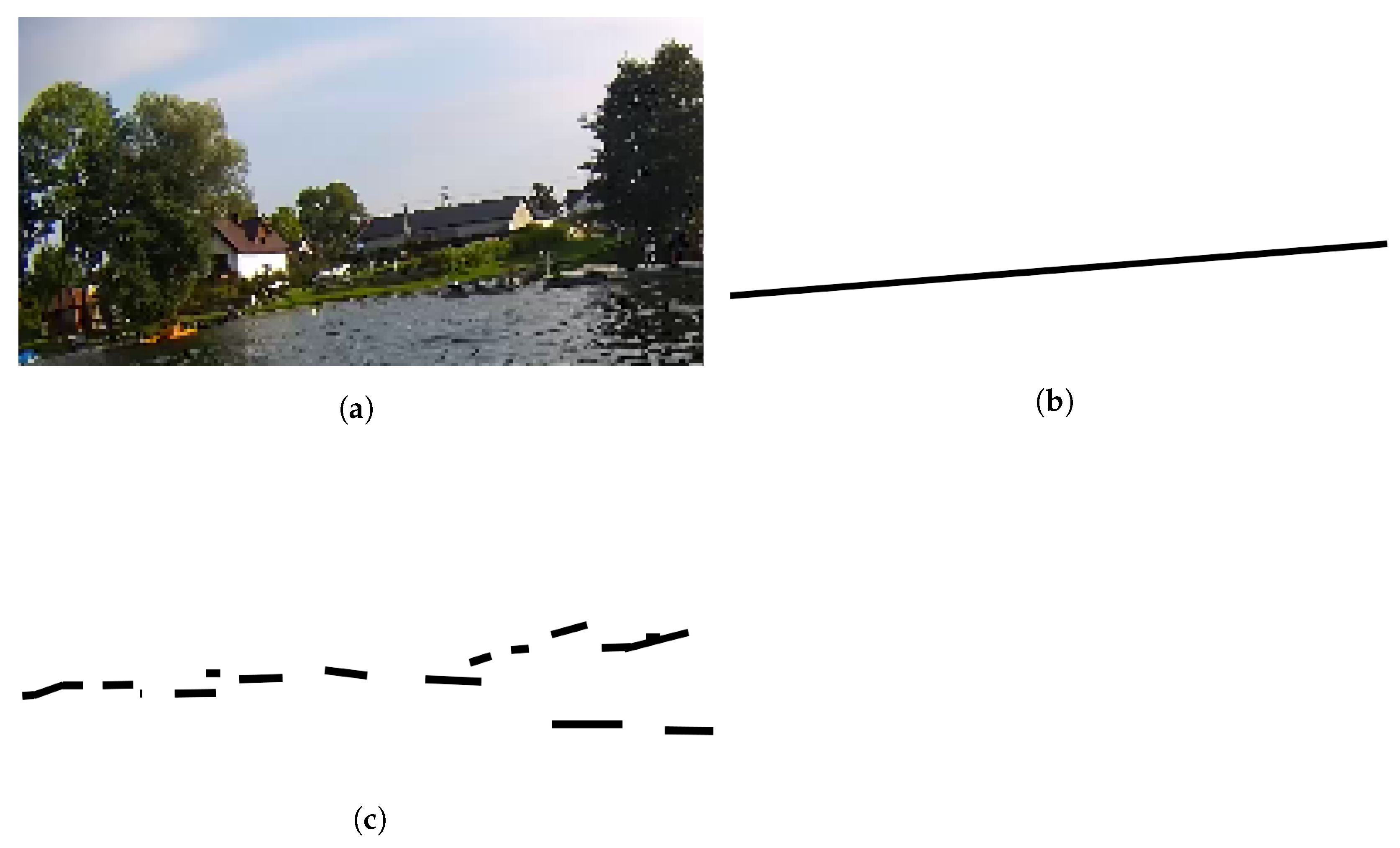
2.2.1. Cropping the Image according to the Selected Methods: Image Processing with Approximation Technique

The classic approach to image analysis assumes the use of graphic filters to obtain specific elements and their subsequent processing. The image should be represented in grayscale, which enables the following Equation [38]:

$$C=0.299·R+0.587·G+0.114·B,$$

(3)

where $[R,G,B]$ stands for selected colors in a given pixel and will be replaced with [C,C,C]. In such a prepared image, the number of elements/objects should be minimized, which can be achieved by using graphic filters by introducing the image convolution operation and the filter matrix. The convolution is based on the principle of modifying the image area and moving it further. Let us mark an image as I, and pixel on position $(x,y)$ with the notation of $I_{x,y}$. Then the convolution can be defined as [39]:

$$k*I_{x,y}=\sum _{i=1}^p\sum _{j=1}^{p}k(i,j)·I_{x+i-1,y+j-1},$$

(4)

where k is a square matrix that stands for a filter. An example is blur defined as $k=\frac{1}{16}\left(\begin{array}{ccc}1& 2& 1\\ 2& 4& 2\\ 1& 2& 1\end{array}\right)$. The next step is to use the edge detection algorithm [40]. The pixels that remain after the use of the algorithm can be used in a linear approximation denoting the shoreline separating the water and the area above it. However, the solution itself is not ideal as it is difficult to estimate the number of uses of individual filters or even combinations of them. The consequence of incorrectly selected processing steps will be too many pixels that points to other objects. A particularly problematic issue is the generalization of this solution into images made with the use of various equipment or parameters.

2.2.2. Cropping the Image according to the Selected Methods: U-Nets

An alternative approach is to use the u-net model, which is a neural network architecture [41]. The network takes the image and returns its modified version. The model assumes the construction of a network with convolution layers (using the Equation (4), but the filter values are found during training), and pooling (reduction of the input image size). Such layers contribute to the extraction of the most important features, which are then used in the image reconstruction process. This occurs through the layers of convolution and up-convolution (the opposite of pooling). The u-net model is trained on a supervised basis, i.e., the network processes the image during training, and verifies the result of the network against the desired modification.

It is a solution that enables fast image processing and automation in the process of finding coefficients. However, it also requires a database for training purposes. In addition, the selection of an architecture may require a lot of testing.

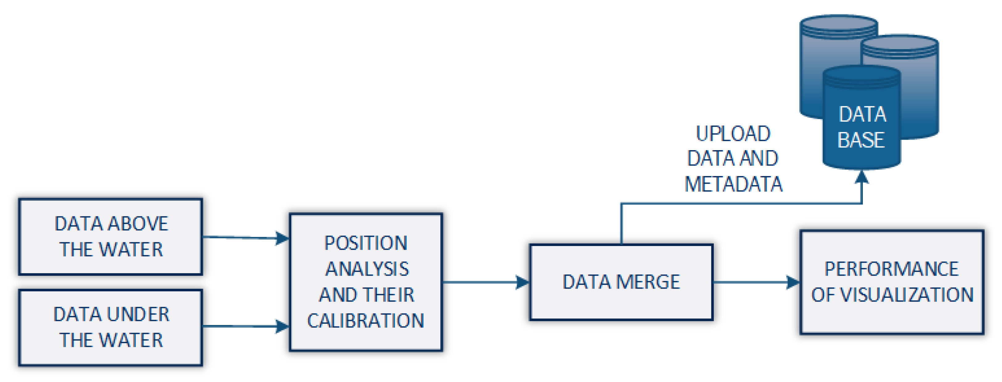
2.3. Data Fusion Based on All Gathered Data

Based on the previously presented ways of processing data from four selected sensors, data fusion is based on their combination. The underwater processing task is the use of a point cloud to generate the surface. Then use the sonar-based mosaic image to apply the texture. In the case of the above-water surface, the situation is similar, as LiDAR generates a cloud of points, which is processed, and then combined with a previously prepared image obtained from the camera. The situation is mainly based on processing this image by removing water areas and approximating the image position to the surface generated from the point cloud. The approximation is based on getting GPS localization of the camera and measured distance to objects using a camera. It should be notice that such georeferencing is the approximated solution that does not guarantee correctness. It is one of the main tasks for future work. However, it can be used for the analysis of objects on the shore, which is described in Section 2.4.

Moreover, creating two surfaces with above-, and underwater areas, they can be placed in one scene after position calibration and scaling (in the case of the wrong scale of images gathered from camera) according to the saved metadata such as a coordinate system. The proposed fusion is based on the overlapping of both areas, however, it is possible to combine point clouds into one, i.e., MBES and LiDAR data. As a result, such action will allow obtaining one surface reflecting the entire measurement area. Unfortunately, this also causes problems with processing data from the camera, where the location of individual pixels is approximated and may contribute to their superimposition in the underwater area. The main idea is to create these two models and then save them in the database. Such action will decrease the number of calculations and allow for further analysis/comparison. A simple visualization is shown in Figure 4. For re-implementation purposes, the proposed solution was also presented in the form of a pseudocode in the Algorithm 1.

2.4. Analysis Module

The created maps based on the data fusion enables various analyzes due to individual data or areas. This is a classic approach to analysis. However, we propose a comparative analysis of two spatial maps made at different time intervals. The result of such measurements will be the detection of changes. An example is making a comparison of the same area. Especially in the case of the analysis of water areas and banks, a change in the landslides of the wharves and cliffs can be noticed. In addition, the analysis of the bottom of the reservoir allows the detection of even the smallest depth changes or littering at the bottom. Hence, it is very important to enable such measurements to be made. The proposed solution is based on a quick analysis of the individual components with overlaying maps.

Such analysis can be made on analysis sub-areas created by dividing the entire measurement environment. Suppose we will divide the area by two axes such as OX and OY into equal rectangles of the same area. Then, having two areas (from different measurements), we have a much smaller number of data to compare and find the differences. However, the greater the number of these sub-areas, the more calculations will be required. In a given area, we can easily determine the maximum or minimum height. Similarly, the case is with the number of points or the amount of coverage of this surface. In the absence of points from one measurement, we quickly receive information about the shift relative to the planned track.

Algorithm 1: Pseudocode of the proposed data processing to obtain chart based on integrated data from various sensors.

Moreover, images like stitched images from cameras can be analyzed by artificial intelligence methods. For this purpose, we use the type of pre-trained convolutional neural network called YOLOv5 [42]. The network returns the probability that detected objects belong to one of the known classes. In this way, you can easily determine the number of buildings around the water reservoir or bridges. In a similar way, we can perform an analysis of sonar images and classify objects such as logs or wrecks.

3. Results

In this section, we evaluate the proposed methodology and compare them to other existing tools and methods. We also analyze the mean time needed to compute all operations in the proposed system. This section was split into three parts: settings description, image processing techniques evaluation and surface creation details with data integration analysis.

3.1. Settings

Sample data for evaluating our proposal were gathered by the lake shore Kłodno in Poland (see Figure 5) and case studies with the comparison were made on lake Zawory in Poland. Data were gathered by HydroDron that is shown in Figure 6. This vessel has GNSS receive which is the source of information about the geographical position of the vessel. It is an auxiliary sensor that allows synchronization of the whole process, both in recording measurement data and creating a spherical projection of panoramic data. The MBES collects bathymetric points in the form of an underwater semi-sphere point cloud. Interferometric sonar PING 3DSS-DX-450 acquires raster images of the bottom. The LiDAR Velodyne VLP-16 (measurements were made at a frequency of 18.08 kHz, in a 30° segment of the vertical plane (the gap between emitter/receiver pairs is $2^{\circ }$) and the entire horizontal plane (for 600 rpm, the resolution is $2^{\circ }$). Laser beam length: 905 nm, field of view 360${}^{\circ }$, maximum range up to 100 m) collects spatial data in the form of a point cloud for objects located in the semi-sphere above the water. The last sensor, the camera Blackfly S GigE-FLIR (model: BFS-PGE-244S8C-C: 24.5 MP, $4096\times 2160$ pixels, pixel depth: 16 bit, 36 g, 5 FPS, Sony IMX540, Color, pixel size: $3.45\times 3.45\mathsf{\mu }$m), takes high-resolution surface images. All evaluations were made in Python 3.9 and the following library: OpenCV, Matplotlib and PyVista [43]. The hardware was Intel Core i9-10850K 3.6 GHz, 32 GB RAM, and MSI GeForce RTX 3060.

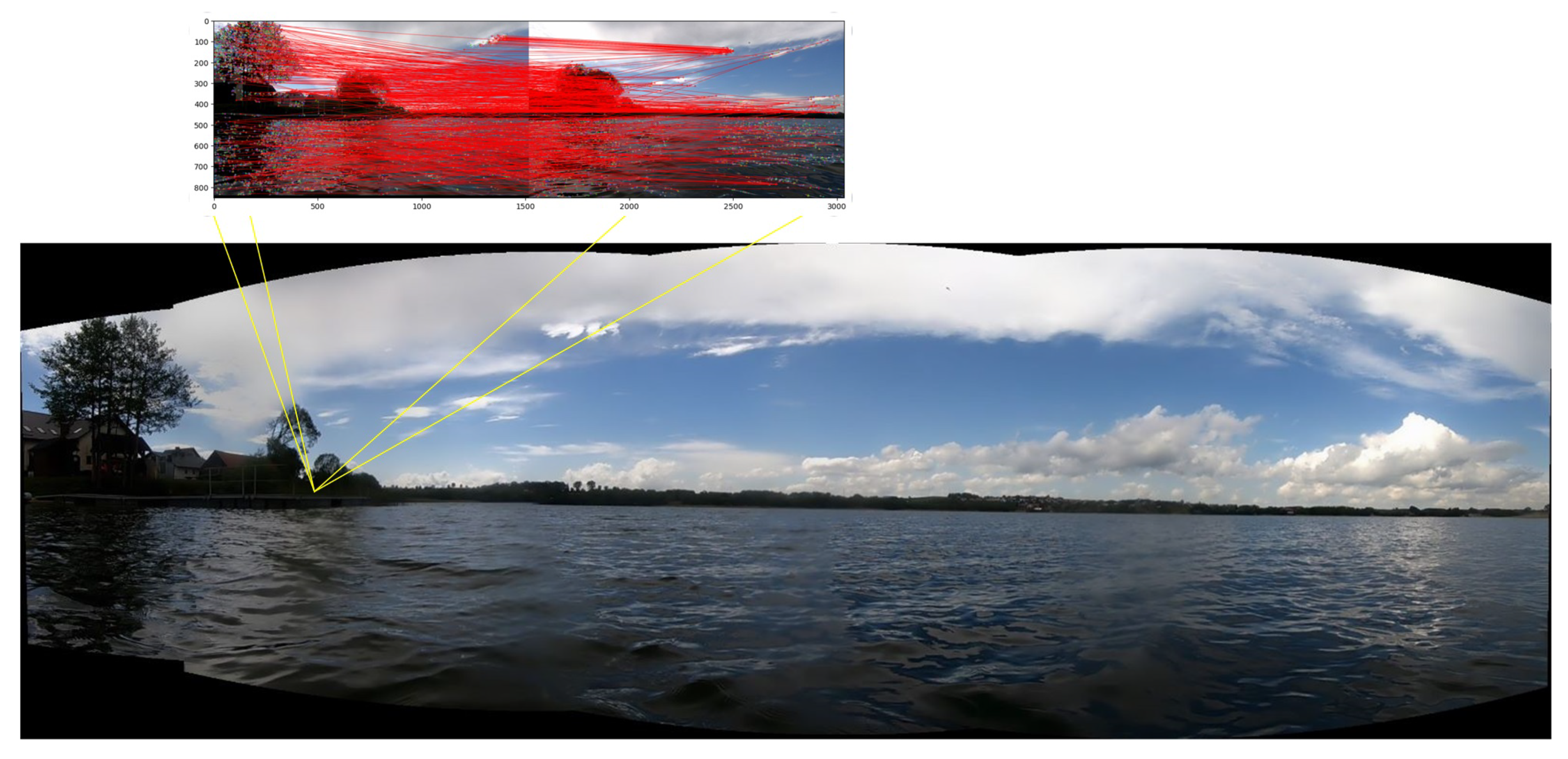
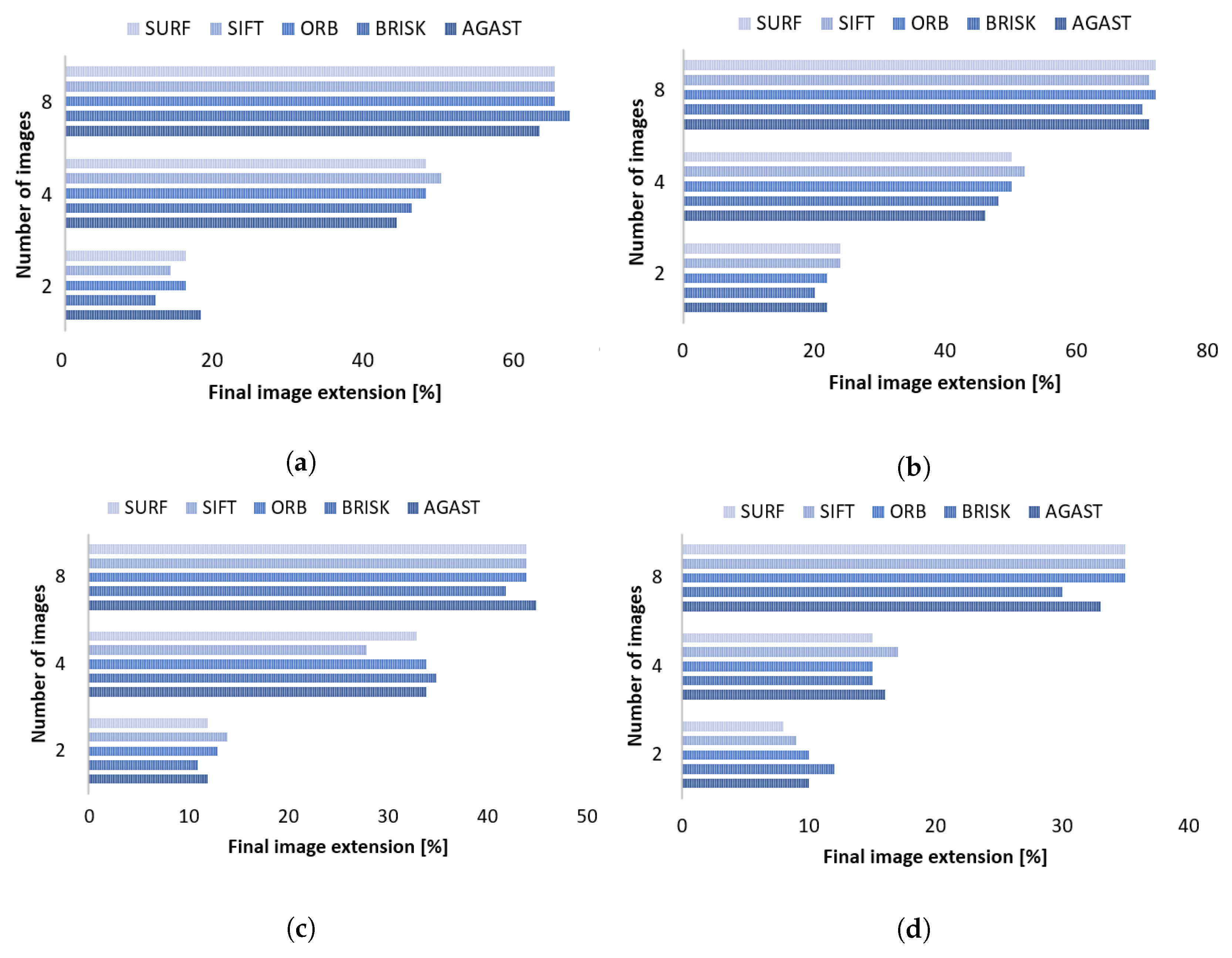
3.2. Image Processing Techniques

At first, we analyzed the method for removing the area above the shore. The size of the recorded video was $960\times 720$ (it was resized due to a large number of calculations). For this purpose, we analyzed different image processing techniques like blur and edge detection. A blur decreases the number of points detected after the edge detection filter, and different numbers of blur filters to remove pixels and edges were applied. The mean slope angle about the shoreline based on 20 different frames is shown in Figure 7. For this purpose, all remaining pixels were used in the linear approximation of the line. The perfect case is $\langle -{10}^{\circ },{10}^{\circ }\rangle$ because of the uneven edge of the shoreline. It could be seen that the results indicated low accuracy because of different weather conditions. On a cloudy day, image processing showed much better adjustment. Another situation was when the image was recorded on a sunny day. Then the sun’s rays were reflected on the water’s surface creating a greater number of detected edges. As a result, the shoreline, after linear interpolation of the remaining pixels, did not match the existing one. The other problem was that there were different objects on shore. This causes many filtering problems. Based on the results, the best-fit line came from a double-blur operation before edge detection.

In parallel, the created image data in the form of pairs (original and with the line) were used to train the u-net. Due to the small training database (based on the performed operations it consisted of 150 samples), we used learning transfer from VGG16 [44,45]. The transfer consists of using the trained values of individual layers and their over-training on a dedicated database. The network architecture processed images of size $512\times 512$, which caused the image to be reduced. We trained the network by 5, 10 and 15, 20 iterations using ADAM algorithm [46] (the simplified architecture model is shown in Figure 8). The network achieved a level accuracy of 80% at 5 iterations. Additional iterations indicated slight fluctuations in the metric, however, the value did not exceed 80.2%. A processed sample by the network is presented in Figure 9. The obtained results indicated that the net results are very ambiguous. It should also be noted that the generous result is subjected to additional image processing (removal of individual pixels and thickening of clusters). The reason for this is that the network returns the white pixels in a black image. The dedicated database was too small for the network to detect the drawn line. An advantage of the solution is the average prediction time, which was 0.13 s based on 10 tests. However, training the network itself is a time-consuming process. Despite the speed of analysis of the samples after training, the accuracy of the network itself as well as the obtained measurements indicate worst results than using classical solutions like image processing.

Next, we investigated the time to perform key-point algorithms and matching results. In the proposal, we suggested a SURF algorithm, but there are others: ORB [30], BRISK [31], AGAST [32] and SIFT [33,34] and simplified SURF [35]. Therefore, we make a comparison to evaluate two things. The first was the mean matching execution time, and the second was an average reduction of image size by matching.

From the few films from which we extracted frames for each second, the tested image size was $1169\times 714$. We evaluated each of them by a selected key-point algorithm according to different $t\in \{1,2,3,4\}$ [second], and 2, 4, 8 images merged into one texture. In

Table 1. Mean time in seconds to process 2, 4 and 8 images with different key-points search algorithms.

	1 s			2 s			3 s			4 s
Number of Images	2	4	8	2	4	8	2	4	8	2	4	8
AGAST	0.11	0.56	1.13	0.11	0.61	1.13	0.16	0.63	1.18	0.21	0.66	1.22
BRISK	0.13	0.66	1.14	0.156	0.71	1.18	0.166	0.75	1.23	0.19	0.75	1.2
ORB	0.12	0.63	1.11	0.133	0.64	1.18	0.162	0.65	1.19	0.18	0.63	1.2
SIFT	0.11	0.55	1.16	0.12	0.6	1.21	0.12	0.64	1.18	0.17	0.61	1.22
SURF	0.12	0.56	1.12	0.14	0.59	1.16	0.17	0.59	1.15	0.18	0.63	1.19

, the mean time for 20 different tests are shown. It is worth noting that the sample processing time was similar due to different frame capture times. However, the fastest average time to process only two images was obtained by SIFT. However, for eight images, SURF and AGAST turned out to be the fastest. In the case of the proposed methodology, the algorithm will have to process many samples; therefore, based on the results, the SURF algorithm was the best choice. In the next step, we focused on the average coverage in relation to the fit. An exemplary fit is shown in Figure 10. It was noted that there was some overwriting of both images, which made cropping necessary. The results of the fit measurements were made by analyzing the extension of the basic image. The results of these measurements are presented in Figure 11a–d. The best ones were obtained for the analysis and the combination of frames shifted in time by two seconds (see Figure 11b). In the case of a combination of eight images, the result expanded by more than 70% for each algorithm. For the combination of four, the image’s width increased by 50%. However, the results for the 1 s time shift (see Figure 11a) returned slightly worse results. When the shift increased to 3 and 4 s, the average coverage for the performed tests reached the maximum of 45% (for $t=3$) and 35% (for $t=4$) because the frames were too far apart, as can be seen in Figure 11c,d. As a result, the algorithms quite often did not find key points that could be used for the combination. It is also worth noting that the images were taken during the turns of the vehicle, which contributed to poorer performance with a higher time shift. For the algorithms, the results were similar, which means each of them is a good approach to creating combined images.

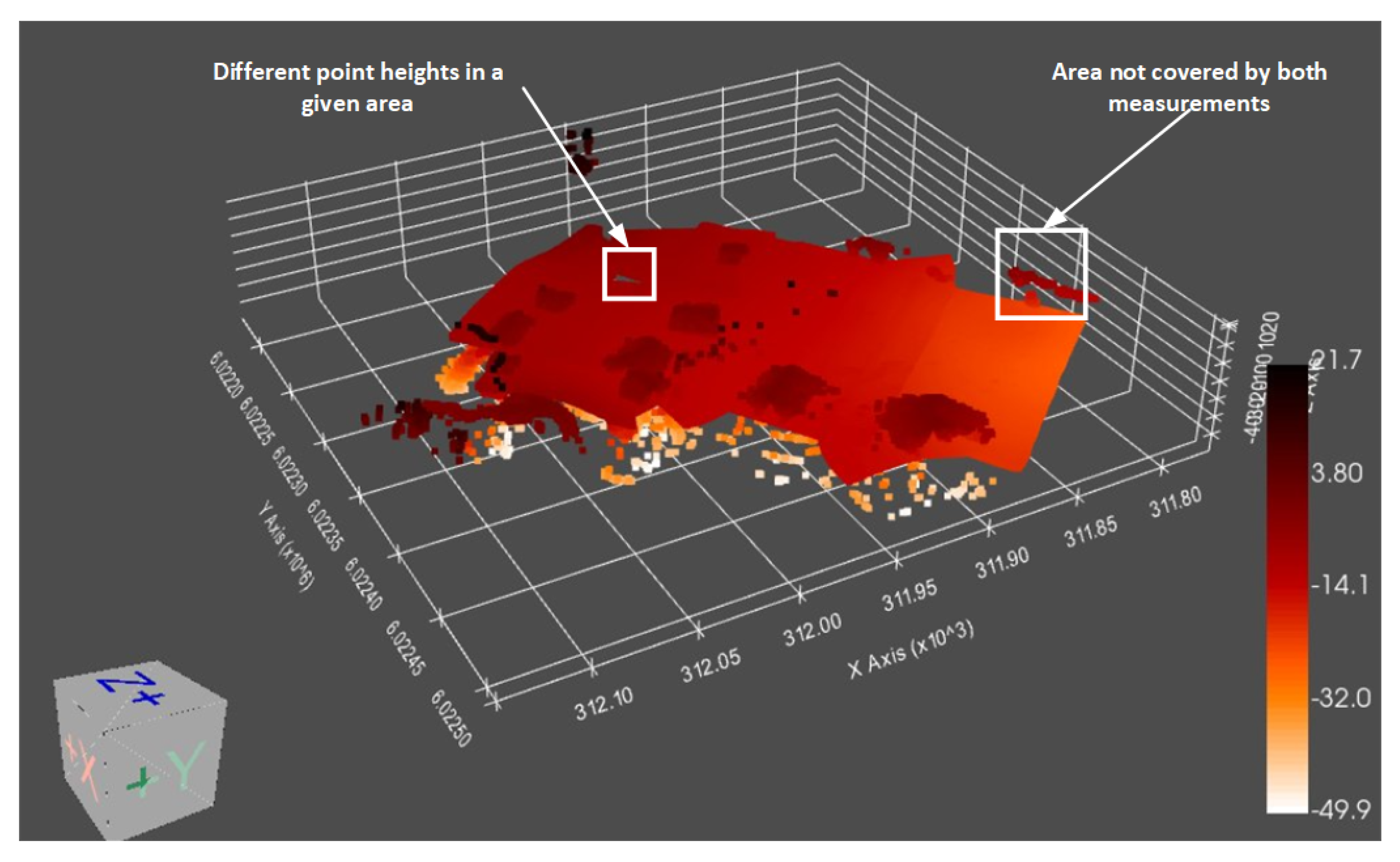
3.3. Surface Creation and Data Integration

The created surface was based on a point cloud that contained more than 5.5 million points. During the experiments, we first analyze the reduction and augmentation. The reduction was based on down-sampling, to reduce the set of points to a certain number. We have evaluated the proposed solution with the analysis of subareas and its post-processing in terms of generating or reducing points. This approach reduces the number of points that need to be processed at any given time as smaller sets are analyzed. However, this is an iterative approach that has achieved similar results in terms of time as shown in

Table 2. Time analysis in processing point cloud data in seconds.

		Number of Points
		100,000	1,000,000	1,000,000
MBES	All data analysis	2049	5374	7143
	Proposed iterative method	2184	5388	7222
LIDAR	All data analysis	2346	5503	6940
	Proposed iterative method	2013	5800	6972

. However, no problem with the RAM limit was detected, as was seen in verifying the verbose data.

3.3.1. Case Study

As part of the comparative analysis tests, two measurements were made nearly three weeks apart on the same reservoir. A water reservoir Zawory on 21 March 2022 and 2 June 2022. Prepared data without imposing textures made it possible to apply them by overlapping. The average value of the area coverage was 81% in terms of MBES and 60% in terms of LiDAR. However, the differences between the imposition were due to analyzes of a larger area than before (see Figure 12). This is due to the expansion of the analysis area and exchanges of the sensors to newer versions. Moreover, the data from 21 March 2022 shows some wrong data measurements due to the wrong reflection when using underwater sensors. As a result, erroneous measurement data exceeding the depth of the water reservoir were obtained. However, the very measurement of the bottom shows slight changes in the shape in selected places. To increase the accuracy of the overlay, the second area on 22 June 2022 was trimmed to the same area as in the previous measurements. 95% overlap was obtained according to MBES data (the analysis was made by dividing the area into 100 sub-areas). The analysis of the bottom surface showed no major differences and small deviations. First of all, slight changes in height at some points were noticed (it can be seen in the marked area in Figure 12). The reason for such actions may be a calibration problem or an obstacle from which the laser beam was reflected. However, changes in height are not regular in a given area, but only in selected points, which are not associated with changes at the bottom. Another observation resulting from the overlaying is related to noticing unanalyzed fragments of the bottom. This is due to the lack of ideal coverage of the area with measurement data due to slight modifications of the ship’s trajectory. Overlay analysis enables surface comparison in terms of points/meshes. However, in future work, we want to focus on the broader development of this analysis by using mass-learning algorithms for segmentation analyses. In addition, the texture is currently an add-on for better visualization. By implicating, textures can allow for a more accurate comparison by detecting individual elements/objects and automatically classifying them through knowledge transfer and the Yolo approach for analysis of not only images but the video.

During the case study (the measurements made in March and June), we notice that there is no easy answer for how many frames should be used to create a stitched image. The measurements were carried out parallel to the shore, where the camera measurement returned about 50% of the rotation, i.e., 180 degrees. 50 frames were used for creating the above-water view, but after reducing them (due to the low-speed value) only 8 would be enough. Moreover, the proposed approximate approach to assigning the camera image to the surface was most often in the wrong places. Based on this research, future work will focus on georeferencing this more accurately.

During conducting experiments, we also trained a YOLOv5 for analyzing camera data. For the purpose of training a set, we created a set composed of two classes: building and bridge. The building set contains 120 training and 35 testing samples (a sample was a frame from a video with the localization of an object). The bridge class has 80 training and 25 testing samples. The results of testing samples were shown as a confusion matrix in Figure 13. Based on the obtained results, for such a small number of training data, the classifier was able to reach 91.7% accuracy. It is a high result taking into account that the classifier was trained by 10 epochs with the ADAM algorithm. Such a trained network was used to evaluate camera data which can be seen in Figure 14. The images show a full model of processed data with the results displayed regarding the sum of buildings and platforms (the object was considered correctly classified when the probability of belonging to the class was a minimum of 80%).

4. Discussion

The modeled solution is based on the end-to-end principle, which is dedicated to automatic, unmanned vessels. This solution allows for obtaining results in the form of visualization and information about the performed measurements. This is a method that can be easily used in intelligent solutions of the Internet of Things, where the introduced methodology enables the processing of big data and subjecting them to comparative analysis with archival data. In Section 3.2, the results related to the image processing are presented. Particular attention was paid to the analysis of frames from the camera. It was noted that the video should be trimmed relative to the frames spaced out by a certain amount of time. The result should be framed that represents part of the area from the previous frame and part of the next frame. Then, there will be a connection between the two frames that can be used for creating a panorama. Various key point analysis algorithms were used to combine these frames. The results for each of the algorithms returned a good combination when the time between frames was 2 s. In addition, it was noticed that the weather or the reflection of light on the water’s surface is an important problem. This type of distortion means that it is not always possible to combine frames due to the lack of the same key points in two images. To minimize the impact of light reflection on the water surface, the use of neural networks was proposed. The u-net model architecture based on VGG was used to create a mask representing the line between the water and the shore. Cropping the frame image helps to minimize the impact of water on key-point analysis. Of course, there are still key points on the clouds that are moving. Hence, it is important not to use too long intervals between frames. Data processing in the form of point clouds focused primarily on sampling and augmentation. The proposed solution made it possible to supplement places where there were fewer points. Such an example was the data at the ends of the areas. In Section 3.3.1, we presented an analysis of the solution based on real data. It was noticed that quick and automatic processing of these data is possible because the results showing the integration of measurements from three sensors and the analysis from the camera were obtained (see Figure 14). An additional element is the created panorama, on which it is possible to find potential objects. Our research focused on the analysis of bridges and buildings. Training of the network was done on a small dataset, however, thanks to the learning transfer, the accuracy was achieved at 91.7%. Apart from data analyses, spatial visualizations indicate the possibility of comparison with archived data. In the case of the study, data from the same area were compared (taken several months apart). In the case of the above water area analysis, the data did not change because no new building or bridge was built. However, bottom surface coverage analysis (see Figure 12) shows a new formation of some mounds of sand.

The conducted experiments proved that it is possible to use various data processing techniques as well as artificial intelligence methods to generate a spherical projection of two panoramic data. In addition, machine learning algorithms have been introduced that allow the removal of water space as well as the classification of objects in the image for their identification. The proposed methodology is dedicated to autonomous water vehicles that are equipped with various sensors that collect data. Based on the performed analyses and the practical use of the solution, attention was paid to the possibilities of data analysis and visualization. This is an interesting approach to analyzing areas concerning changing conditions on the shore as well as the bottom itself. The proposed solution allows for the automatic processing of the acquired data, which is an asset. It is worth noting that currently there is similar software like Ocean Alpha or Seabots. Our proposition distinguishes itself primarily by the method of data processing, as well as the possibilities of analyzing the data itself and the selection of sensors, which we plan to expand in the future. Moreover, many directions of software development have also been noticed. In future work, we plan to extend our proposition with other data and improve the performance of the current proposal. We especially want to focus on finding the solution for correct georeferencing the camera image to the LiDAR surface and extending the analysis module, which can be improved by segmentation or analysis of sonar images.

5. Conclusions

In this paper, we presented operating schemes that combined data from different sensors. We have proposed to separate above- and under-water data to generate separate 3D models and aggregate them later. As part of the research, we have tested individual components in processing collected data from different sensors like multibeam echosounder, 3D side-scan sonar, and mobile laser scanner supported by video images subjected to sensory fusion. The modeled solution is based on the processing of individual data in order to create a visualization combined with the obtained measurement data. As part of the research, attention was paid to the possibility of obtaining insufficient or too much data. The final representation of the results enables data visualization with the support of the research analysis module, an example of which is the use of machine learning methods. It is a solution built as an end-to-end application, where the acquired measurement data is automatically processed and displayed to the user. Conducted experiments in terms of image processing tools consisting of the classic key-point algorithm to generate panoramic images composed of many video frames. Different time intervals between video frames were tested, where for 2 frames the fastest was SIFT. In the case of 8 frames, the shortest time needed to merge frames was obtained by SURF and AGAST. As part of this research, attention was paid to the combination of the images and how much enlargement of the image was acquired. The best results were achieved when 8 frames were combined 2 s apart, which allowed obtaining over 70% expansion. Image analysis using a trained convolutional network for two classes reached an accuracy of 91.7%. In addition, problems were noticed with shoreline detection, which is dependent on the prevailing weather conditions (with the use of classic image processing tools and u-net). In the case of point cloud analysis, a solution has been proposed that allows automatically checking whether there are too many or too few points in a given area. This is due to the situation when there is an error in the measurements. The modeled mechanism enables automatic analysis of the number of points in smaller subareas and then performing augmentation or reduction of points. It is worth noting that the use of four sensors for obtaining measurement data has enabled the creation of a real visualization model and undergoing quick analysis. As part of the research and modeled framework, two data analysis methods were prepared. The first was to compare data from the selected type by imposing and detecting changes to archival data. The second was the use of neural networks for classification, which allows quick classification of objects and their statistical comparison. Both forms of analysis allow searching for other types of changes, which increases the possibilities of its extension and use in practical needs.

References

1. Wawrzyniak, N.; Hyla, T.; Bodus-Olkowska, I. Vessel identification based on automatic hull inscriptions recognition. PLoS ONE 2022, 17, e0270575. [Google Scholar] [CrossRef] [PubMed]
2. Trigg, A. Geospatial Data Integration: Panacea or Nightmare? Int. Arch. Photogramm. Remote Sens. 1997, 32, 333–340. [Google Scholar]
3. Manoj, M.; Dhilip Kumar, V.; Arif, M.; Bulai, E.R.; Bulai, P.; Geman, O. State of the art techniques for water quality monitoring systems for fish ponds using iot and underwater sensors: A review. Sensors 2022, 22, 2088. [Google Scholar] [CrossRef] [PubMed]
4. Hoegner, L.; Abmayr, T.; Tosic, D.; Turzer, S.; Stilla, U. Fusion of 3D point clouds with tir images for indoor scene reconstruction. Int. Arch. Photogramm. Remote Sens. Spat. Inf. Sci. 2018, 42, 5194. [Google Scholar] [CrossRef] [Green Version]
5. Fujimura, S.; Kiyasu, S. A feature extraction scheme for qualitative and quantitative analysis from hyperspectral data-data integration of hyperspectral data. Int. Arch. Photogramm. Remote Sens. 1997, 32, 74–79. [Google Scholar]
6. Honikel, M. Improvement of InSAR DEM accuracy using data and sensor fusion. In International Geoscience and Remote Sensing Symposium; Institute of Electrical & Electronicsengineers, Inc. (IEE): Piscataway, NJ, USA, 1998; Volume 5, pp. 2348–2350. [Google Scholar]
7. Wang, X.; Yang, F.; Zhang, H.; Su, D.; Wang, Z.; Xu, F. Registration of Airborne LiDAR Bathymetry and Multibeam Echo Sounder Point Clouds. IEEE Geosci. Remote Sens. Lett. 2021, 19, 1–5. [Google Scholar] [CrossRef]
8. Skovgaard Andersen, M.; Øbro Hansen, L.; Al-Hamdani, Z.; Schilling Hansen, S.; Niederwieser, M.; Baran, R.; Steinbacher, F.; Brandbyge Ernstsen, V. Mapping shallow water bubbling reefs-a method comparison between topobathymetric lidar and multibeam echosounder. In Proceedings of the EGU General Assembly Conference Abstracts, Online, 19–30 April 2021; p. EGU21-15899. [Google Scholar]
9. Shang, X.; Zhao, J.; Zhang, H. Obtaining high-resolution seabed topography and surface details by co-registration of side-scan sonar and multibeam echo sounder images. Remote Sens. 2019, 11, 1496. [Google Scholar] [CrossRef] [Green Version]
10. Li, J.; Qin, H.; Wang, J.; Li, J. OpenStreetMap-based autonomous navigation for the four wheel-legged robot via 3D-Lidar and CCD camera. IEEE Trans. Ind. Electron. 2021, 69, 2708–2717. [Google Scholar] [CrossRef]
11. Kunz, C.; Singh, H. Map building fusing acoustic and visual information using autonomous underwater vehicles. J. Field Robot. 2013, 30, 763–783. [Google Scholar] [CrossRef] [Green Version]
12. Xie, S.; Pan, C.; Peng, Y.; Liu, K.; Ying, S. Large-scale place recognition based on camera-lidar fused descriptor. Sensors 2020, 20, 2870. [Google Scholar] [CrossRef]
13. Hartling, S.; Sagan, V.; Sidike, P.; Maimaitijiang, M.; Carron, J. Urban tree species classification using a WorldView-2/3 and LiDAR data fusion approach and deep learning. Sensors 2019, 19, 1284. [Google Scholar] [CrossRef] [PubMed] [Green Version]
14. Shin, Y.S.; Park, Y.S.; Kim, A. Direct visual slam using sparse depth for camera-lidar system. In Proceedings of the 2018 IEEE International Conference on Robotics and Automation (ICRA), Brisbane, Australia, 21–25 May 2018; pp. 5144–5151. [Google Scholar]
15. Subedi, D.; Jha, A.; Tyapin, I.; Hovland, G. Camera-lidar data fusion for autonomous mooring operation. In Proceedings of the 2020 15th IEEE Conference on Industrial Electronics and Applications (ICIEA), Kristiansand, Norway, 9–13 November 2020; pp. 1176–1181. [Google Scholar]
16. Wang, M.; Wu, Z.; Yang, F.; Ma, Y.; Wang, X.H.; Zhao, D. Multifeature extraction and seafloor classification combining LiDAR and MBES data around Yuanzhi Island in the South China Sea. Sensors 2018, 18, 3828. [Google Scholar] [CrossRef] [PubMed] [Green Version]
17. De Silva, V.; Roche, J.; Kondoz, A. Robust fusion of LiDAR and wide-angle camera data for autonomous mobile robots. Sensors 2018, 18, 2730. [Google Scholar] [CrossRef] [Green Version]
18. Ge, C.; Du, Q.; Li, W.; Li, Y.; Sun, W. Hyperspectral and LiDAR data classification using kernel collaborative representation based residual fusion. IEEE J. Sel. Top. Appl. Earth Obs. Remote Sens. 2019, 12, 1963–1973. [Google Scholar] [CrossRef]
19. Liu, H.; Yao, Y.; Sun, Z.; Li, X.; Jia, K.; Tang, Z. Road segmentation with image-LiDAR data fusion in deep neural network. Multimed. Tools Appl. 2020, 79, 35503–35518. [Google Scholar] [CrossRef]
20. Hu, C.; Wang, Y.; Yu, W. Mapping digital image texture onto 3D model from LiDAR data. Int. Arch. Photogramm. Remote Sens. Spat. Inf. Sci. 2008, 37, 611–614. [Google Scholar]
21. Dąbrowska, D.; Witkowski, A.; Sołtysiak, M. Representativeness of the groundwater monitoring results in the context of its methodology: Case study of a municipal landfill complex in Poland. Environ. Earth Sci. 2018, 77, 1–23. [Google Scholar] [CrossRef] [Green Version]
22. Blachnik, M.; Sołtysiak, M.; Dąbrowska, D. Predicting presence of amphibian species using features obtained from gis and satellite images. ISPRS Int. J. Geo-Inf. 2019, 8, 123. [Google Scholar] [CrossRef] [Green Version]
23. Toth, C.K.; Grejner-Brzezinska, D.A. Performance analysis of the airborne integrated mapping system (AIMS). Int. Arch. Photogramm. Remote Sens. 1997, 32, 320–326. [Google Scholar]
24. Li, R.; Wang, W.; Tu, Z.; Tseng, H.Z. Object recognition and measurement from mobile mapping image sequences using Hopfield neural networks: Part II. Int. Arch. Photogramm. Remote Sens. 1997, 32, 192–197. [Google Scholar]
25. Chen, Y.; Hu, V.T.; Gavves, E.; Mensink, T.; Mettes, P.; Yang, P.; Snoek, C.G. Pointmixup: Augmentation for point clouds. In Proceedings of the European Conference on Computer Vision, Glasgow, UK, 23–28 August 2020; Springer: Berlin/Heidelberg, Germany, 2020; pp. 330–345. [Google Scholar]
26. Szlobodnyik, G.; Farkas, L. Data augmentation by guided deep interpolation. Appl. Soft Comput. 2021, 111, 107680. [Google Scholar] [CrossRef]
27. Li, L.; Heizmann, M. 2.5D-VoteNet: Depth map based 3D object detection for real-time applications. In Proceedings of the British Machine Vision Conference, Online, 22–25 November 2021. [Google Scholar]
28. Li, Q.; Nevalainen, P.; Peña Queralta, J.; Heikkonen, J.; Westerlund, T. Localization in unstructured environments: Towards autonomous robots in forests with delaunay triangulation. Remote Sens. 2020, 12, 1870. [Google Scholar] [CrossRef]
29. Xu, X.; Li, J.; Zhou, M. Delaunay-triangulation-based variable neighborhood search to solve large-scale general colored traveling salesman problems. IEEE Trans. Intell. Transp. Syst. 2020, 22, 1583–1593. [Google Scholar] [CrossRef]
30. Rublee, E.; Rabaud, V.; Konolige, K.; Bradski, G. ORB: An efficient alternative to SIFT or SURF. In Proceedings of the 2011 International conference on computer vision, Washington, DC, USA, 6–13 November 2011; pp. 2564–2571. [Google Scholar]
31. Leutenegger, S.; Chli, M.; Siegwart, R.Y. BRISK: Binary robust invariant scalable keypoints. In Proceedings of the 2011 International conference on computer vision, Washington, DC, USA, 6–13 November 2011; pp. 2548–2555. [Google Scholar]
32. Zhang, H.; Wohlfeil, J.; Grießbach, D. Extension and evaluation of the AGAST feature detector. In Proceedings of the XXIII ISPRS Congress Annals 2016, Prague, Czech Republic, 12–19 July 2016; Volume 3, pp. 133–137. [Google Scholar]
33. Lindeberg, T. Scale Invariant Feature Transform; KTH Royal Institute of Technology: Stockholm, Sweden, 2012; Volume 7, p. 10491. [Google Scholar]
34. Wang, Y.; Du, L.; Dai, H. Unsupervised SAR image change detection based on SIFT keypoints and region information. IEEE Geosci. Remote Sens. Lett. 2016, 13, 931–935. [Google Scholar] [CrossRef]
35. Bay, H.; Tuytelaars, T.; Gool, L.V. Surf: Speeded up robust features. In Proceedings of the European Conference on Computer Vision, Graz, Austria, 7–13 May 2006; pp. 404–417. [Google Scholar]
36. Villar, S.A.; Rozenfeld, A.; Acosta, G.G.; Prados, R.; García, R. Mosaic construction from side-scan sonar: A comparison of two approaches for beam interpolation. In Proceedings of the 2015 IEEE/OES Acoustics in Underwater Geosciences Symposium (RIO Acoustics), Rio de Janeiro, Brazil, 29–31 July 2015; pp. 1–8. [Google Scholar]
37. Zhan, W.; Xiao, C.; Wen, Y.; Zhou, C.; Yuan, H.; Xiu, S.; Zou, X.; Xie, C.; Li, Q. Adaptive semantic segmentation for unmanned surface vehicle navigation. Electronics 2020, 9, 213. [Google Scholar] [CrossRef] [Green Version]
38. Bala, R.; Braun, K.M. Color-to-grayscale conversion to maintain discriminability. In Proceedings of the Color Imaging IX: Processing, Hardcopy, and Applications, San Jose, CA, USA, 18 January 2003; Volume 5293, pp. 196–202. [Google Scholar]
39. Kim, S.; Casper, R. Applications of Convolution in Image Processing with MATLAB; University of Washington: Seattle, WA, USA, 2013; pp. 1–20. [Google Scholar]
40. Peli, T.; Malah, D. A study of edge detection algorithms. Comput. Graph. Image Process. 1982, 20, 1–21. [Google Scholar] [CrossRef]
41. Siddique, N.; Paheding, S.; Elkin, C.P.; Devabhaktuni, V. U-net and its variants for medical image segmentation: A review of theory and applications. IEEE Access 2021, 9, 82031–82057. [Google Scholar] [CrossRef]
42. Huang, T.; Cheng, M.; Yang, Y.; Lv, X.; Xu, J. Tiny Object Detection based on YOLOv5. In Proceedings of the 2022 the 5th International Conference on Image and Graphics Processing (ICIGP), Beijing, China, 7–9 January 2022; pp. 45–50. [Google Scholar]
43. Sullivan, C.; Kaszynski, A. PyVista: 3D plotting and mesh analysis through a streamlined interface for the Visualization Toolkit (VTK). J. Open Source Softw. 2019, 4, 1450. [Google Scholar] [CrossRef]
44. Ghosh, S.; Chaki, A.; Santosh, K. Improved U-Net architecture with VGG-16 for brain tumor segmentation. Phys. Eng. Sci. Med. 2021, 44, 703–712. [Google Scholar] [CrossRef]
45. Kanaeva, I.; Ivanova, J.A. Road pavement crack detection using deep learning with synthetic data. In Proceedings of the IOP Conference Series: Materials Science and Engineering, Sanya, China, 12–14 November 2021; Volume 1019, p. 012036. [Google Scholar]
46. Zhang, Z. Improved adam optimizer for deep neural networks. In Proceedings of the 2018 IEEE/ACM 26th International Symposium on Quality of Service (IWQoS), Banff, AB, Canada, 4–6 June 2018; pp. 1–2. [Google Scholar]
Figure 1. In the proposed underwater data fusion model, sonar data are combined with point cloud (MBES). The sonar data are processed to create a texture to be used to cover the surface created from a reduced point cloud.
Remotesensing 15 01763 g001
Figure 2. Side-scan sonar processing by deleting the dead zone.
Remotesensing 15 01763 g002
Figure 3. The proposed above-water data fusion model is based on the creation of a stitched image from video files, a surface is created by the use of the Delaunay triangulation method on augmented LiDAR data.
Remotesensing 15 01763 g003
Figure 4. Visualization of the final operation of the proposed method. The combination of the underwater and surface maps is done by using the georeferencing of point clouds and their possible calibration. The map is saved in a database for a specific area, which with more maps can be used to compare and analyze changes.
Remotesensing 15 01763 g004
Figure 5. Measurement settings, (a) Covered area (Zawory, Poland) with sensors and visualized with Hypack 2022 software, (b) Image was taken while taking measurements.
Remotesensing 15 01763 g005
Figure 6. Sensors mounted on an autonomous unmanned hydrographic vessel: 1—global navigation satellite system (GNSS) receiver, 2—multibeam echosounder (MBES), 3—sonar, 4—light detection and ranging (LiDAR), 5—camera.
Remotesensing 15 01763 g006
Figure 7. Graph of the dependence of the number of blur filter applications against the slope of the shoreline under selected weather conditions.
Remotesensing 15 01763 g007
Figure 8. VGG-based u-net architecture, where the gray blocks are the transfer from VGG16.
Remotesensing 15 01763 g008
Figure 9. Obtained result from u-net. (a) Orginal image, (b) Line obtained by classic image processing techniques and approximation, (c) U-net result after deleting single pixels and bold clusters.
Remotesensing 15 01763 g009
Figure 10. The effect of using the key point detection algorithm and the superimposition of images through the located points on two frames within 2 s.
Remotesensing 15 01763 g010
Figure 11. Mean execution time of key point algorithms for processing a given number of frames cut relative to a given period of time, (a) 1 s, (b) 2 s, (c) 3 s, (d) 4 s.
Remotesensing 15 01763 g011
Figure 12. Overlaying the measurement data to identify changes. The visualization was created on the basis of the analysis of data collected on 21 March 2022 and 2 June 2022 on a water reservoir Zawory in Poland.
Remotesensing 15 01763 g012
Figure 13. Confusion matrix on the testing set.
Remotesensing 15 01763 g013
Figure 14. An example of created panorama and visualization based on obtained measurement data with an analysis of current measurements using machine learning, not imposing data. On the left, results with created sonar mosaic, and on the right without sonar data.
Remotesensing 15 01763 g014