Article

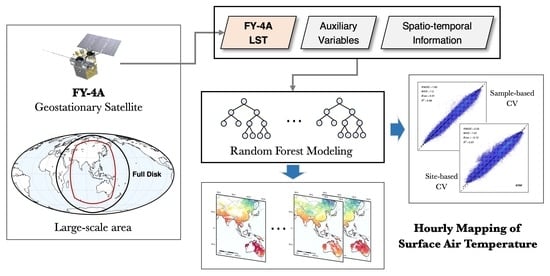
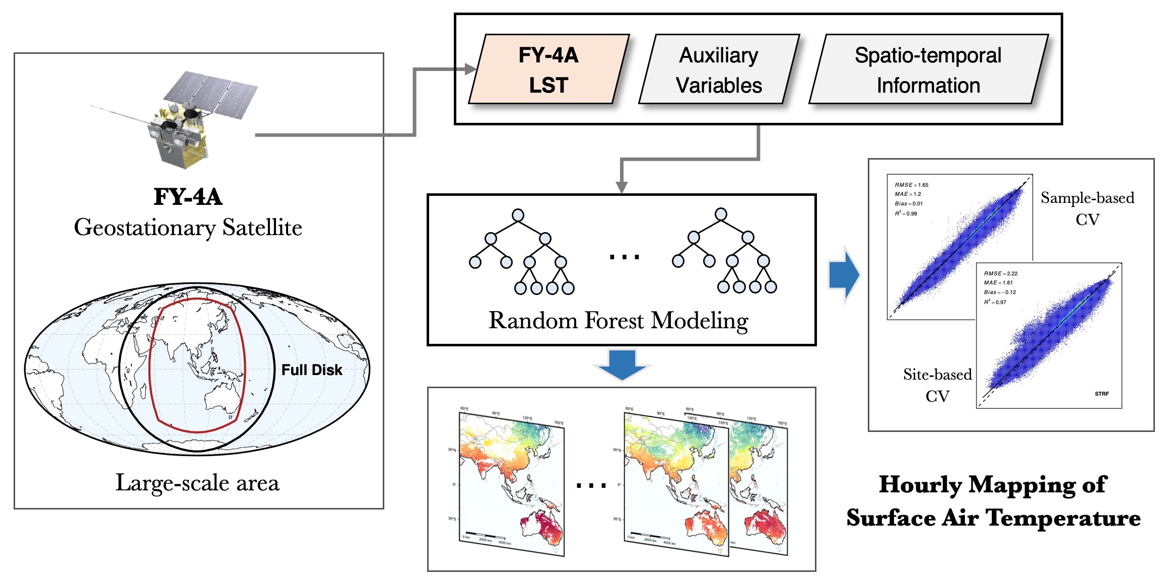
Large-Scale Estimation of Hourly Surface Air Temperature Based on Observations from the FY-4A Geostationary Satellite

1
School of Remote Sensing and Geomatics Engineering, Nanjing University of Information Science and Technology, Nanjing 210044, China
2
Technology Innovation Center for Integration Applications in Remote Sensing and Navigation, Ministry of Natural Resources, Nanjing 210044, China
3
Jiangsu Province Engineering Research Center of Collaborative Navigation/Positioning and Smart Application, Nanjing University of Information Science and Technology, Nanjing 210044, China
4
School of Resources and Environmental Science, Wuhan University, Wuhan 430079, China
5
Beijing Key Laboratory of Urban Spatial Information Engineering, Beijing Institute of Surveying and Mapping, Beijing 100038, China
*
Author to whom correspondence should be addressed.
Remote Sens. 2023, 15(7), 1753; https://doi.org/10.3390/rs15071753
Submission received: 29 January 2023 / Revised: 22 March 2023 / Accepted: 23 March 2023 / Published: 24 March 2023
(This article belongs to the Special Issue Thermal Remote Sensing for Monitoring Terrestrial Environment)

Abstract

:
Spatially continuous surface air temperature (SAT) is of great significance for various research areas in geospatial communities, and it can be reconstructed by the SAT estimation models that integrate accurate point measurements of SAT at ground sites with wall-to-wall datasets derived from remotely sensed observations of spaceborne instruments. As land surface temperature (LST) strongly correlates with SAT, estimation models are typically developed with LST as a primary input. Geostationary satellites are capable of observing the Earth’s surface across large-scale areas at very high frequencies. Compared to the substantial efforts to estimate SAT at daily or monthly scales using LST derived from MODIS, very limited studies have been performed to estimate SAT at high-temporal scales based on LST from geostationary satellites. Estimation models for hourly SAT based on the LST derived from FY-4A, the first geostationary satellite in China’s new-generation meteorological observation mission, were developed for the first time in this study. The models were fully cross-validated for a very large-scale region with diverse geographic settings using random forest, and specified differently to explore the influence of time and location variables on model performance. Overall predictive performance of the models is about 1.65–2.08 K for sample-based cross-validation, and 2.22–2.70 K for site-based cross-validation. Incorporating time or location variables into the hourly models significantly improves predictive performance, which is also confirmed by the analysis of predictive errors at temporal scales and across sites. The best-performing model with an average RMSE of 2.22 K was utilized for reconstructing maps of SAT for each hour. The hourly models developed in this study have general implications for future studies on large-scale estimating of hourly SAT based on geostationary LST datasets.

Graphical Abstract

1. Introduction

Surface air temperature (SAT), a key meteorological element, is routinely measured at weather stations by thermometers mounted about 2.5 m above the ground. Networks of ground weather stations operated around the world provide high-quality, point-scale measurements at high temporal scales, from which many observational data products have been developed with strict quality assurance measures. Observational products for site observations are crucial for a variety of research disciplines, such as climate studies [1]. For example, GHCN (Global Historical Climatology Network) datasets, containing both daily and monthly air temperature measurements, were generated by assembling large numbers of station records from various sources [2,3]. However, ground weather stations or observational data products only provide point measurements of SAT at stations, representing thermal states of the ambient atmosphere around the stations. Point measurements from scarce and unevenly distributed ground sites are difficult to use to quantify complex spatiotemporal patterns of SAT over large-scale areas, especially over areas with complex topographic features and a wide range of geographic settings. Very limited weather stations are installed and operated in the areas with harsh environments, such as mountainous regions, and thus the atmospheric conditions of these areas are severely undersampled by observations from weather stations. In contrast to point measurements of SAT, spatially continuous SAT provides an important data source for many studies, such as urban heat islands [4], exposure to heatwaves [5] and assessment of local climate [1], and has also been used to drive local land surface numerical models [6,7].
Remote sensing techniques have the superior advantage of continuously scanning the atmosphere and Earth surfaces over large-scale areas at regular periods using scientific instruments onboard satellites. In particular, spaceborne multispectral imaging sensors configured with split-window channels in the thermal infrared (TIR) spectrum can produce wall-to-wall TIR radiative observations for characterizing thermal states of land surface. TIR observations are typically used to derive land surface temperature (LST), which is strongly associated with ground-observed SAT [8,9]. Thus, spatially continuous SAT can be reconstructed at high spatial resolutions by integrating accurate point measurements of SAT from weather station and TIR observations from satellites [10,11]. LST, together with auxiliary spatial variables, has been widely used as the primary input variable for SAT estimation models for reconstructing spatial fields of SAT. It is worth noting that original calibrated radiative observations from TIR bands can also be used directly for developing estimation models [12]. SAT estimation models are built on the statistical relationships between ground-observed SAT and these spatial variables at sites. Previous studies have developed SAT estimation models using various methods, which can be generally classified into three categories, including the TVX (temperature vegetation index) methods, parametric methods of energy balance and methods based on statistical learning algorithms [13].
The TVX method is based on the assumption that air temperature of a vegetation canopy is approximated as the surface temperature of the canopy, and estimates SAT of a ground pixel using the relationship between LST and vegetation index, which is calibrated from paired samples in a neighboring window around the pixel [13,14]. As the validity of TVX severely depends on the temperature–vegetation relation, the method is limited to areas with high spatially variable vegetation coverage [9]. Robustness of fitting the relation is further impacted by the number of paired samples in a neighboring window [15]. Estimation models based on energy balance estimate the SAT for each pixel using a physically parameterized energy process between land surface and ambient atmosphere. The satellite-derived LST was used as a key input for the parameterized energy balance models [16,17]. As deriving representative parameterizations of energy processes at finer scales is difficult, this method is seldom applied for estimating SAT. In contrast, SAT estimation models have been extensively developed using various statistical methods or learning algorithms, such as linear regression [18], fixed effect regression [19], spatially explicit regression [20,21], Bayesian spatial modeling [11], ensemble learning algorithms [22,23,24] and neural networks [25]. Statistical learning algorithms have great flexibility and high capability in modeling nonlinear relationships and have received increasing popularity in estimating SAT in recent years. Although deep learning techniques have been applied for SAT estimation in a recent study [25], deep learning is more suitable for inherently complex modeling tasks with huge amounts of labeled samples and high-dimensional input features, such as computer vision and natural language processing [26]. Additionally, we should note that there is no absolutely best-performing learning algorithm for all modeling tasks under all scenarios. Predictive capabilities of the SAT estimation models developed using learning algorithms not only depend on the types of algorithms, but also is affected by the tuning of algorithm parameters, settings of hyperparameters of the algorithms, scales of study areas, and selection of input features for modeling of SAT. However, conventional machine learning algorithms, such as random forest and gradient boosting, are adequate for the modeling task involved in SAT estimation, considering the complexity and characteristics of data samples involved in the tasks [27].
Although substantial studies have been performed to estimate SAT using various methods, these studies are primarily focused on introducing new statistical methods or comparing between different learning methods. In addition, previous studies are predominantly based on the LST retrieved from MODIS for estimating daily and monthly SAT. For example, a recent study [28] has also used MODIS LST for estimating monthly SAT over the United Arab Emirates. MODIS is the multispectral sensor mounted on NASA’s polar-orbiting satellites Terra and Aqua, which have been acquiring Earth observation data since about 2000 and will soon be decommissioned. Many countries and agencies across the world are developing and maintaining their spaceborne Earth observation systems of satellites, resulting in comprehensive systems of Earth observation satellites. Thus, there is a need to extend and facilitate the studies for SAT estimation based on the diverse TIR observations and corresponding LST data products from the satellite systems. In this regard, Zhang and Du [29] developed an ensemble of models for estimating daily SAT using LST datasets from the new-generation meteorological satellite missions, including NOAA’s JPSS and EUMETSAT’s EPS. Imaging sensors onboard geostationary satellites can scan a large-scale region at very high frequencies. Few studies have been carried out to estimate SAT at high temporal scales using the observations from geostationary satellites, and most are based on the LST derived from the SEVIRI sensor mounted on MSG geostationary satellites. In these studies, different methods have been used to develop high-temporal SAT estimation models, such as the TVX methods [30,31], parameterized energy process models [16] and statistical learning [12,32,33]. Recently, a study for hourly SAT [27] has developed hourly SAT estimation models based on LST datasets from the GOES-R meteorological geostationary satellites. However, compared to the substantial studies for estimating daily SAT, the studies for estimating high-temporal SAT using geostationary observations is severely limited, and moreover, the existing studies for estimating high-temporal SAT are limited to small-scale areas. FY-4 (Fengyun), China’s new-generation geostationary meteorological satellite mission [34], is now in operational orbits as a twin satellite system including FY-4A and FY-4B for routinely observing over Asia and Oceania, but there are no studies for developing an estimation model for high-temporal SAT using the LST derived from TIR observations of the FY-4 satellites.
In this study, we developed hourly SAT estimation models based on the LST derived from FY-4A TIR observations to obtain spatially continuous SAT at an hourly scale. The estimation models were developed with a very large number of stations for a very large-scale region contained in the observation coverage of FY-4A’s full-disk. Random forest, a popular ensemble learning algorithm with great capabilities in nonlinear complex modeling tasks, was adopted to develop the hourly estimation models with the FY-4A LST as the primary input. Variables related to time and location are important in spatial modeling tasks, and to explore the influence of the variables on predictive performance of hourly SAT models, four hourly estimation models were specified, including a baseline model and three other models additionally incorporating the time or location variables. Predictive performance of the four specified hourly models was assessed using cross-validation approaches. Overall model performance and model predictive errors at temporal scales and across sites were analyzed and compared between different models. The estimation model with the highest performance was then utilized to reconstruct hourly maps of SAT over the study area. As LST retrievals contain many missing pixels due to cloud contamination that result in missing estimates in the hourly maps of SAT, data coverage of the estimated hourly SAT was analyzed.

2. Materials and Methods
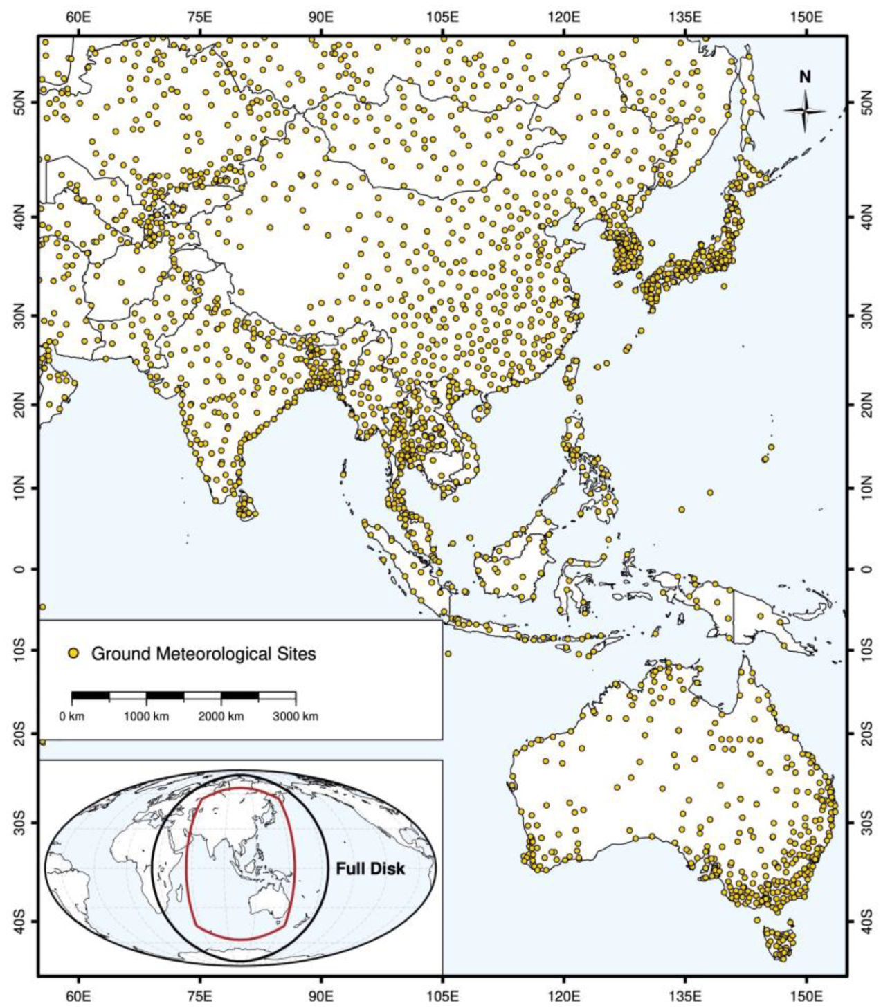
2.1. Study Area

We developed SAT estimation models for the land areas, which are contained in a very large-scale geographic extent with longitudes ranging from 55°E to 255°E and latitudes ranging from 45°S to 55°N (Figure 1).
The spatial extent of the study areas was selected based on the full-disc observation coverage of the FY-4A satellite, which is located at 104.7°E above the Equator. The full-disc of FY-4A, as indicated by the black line in the inset map of Figure 1, encompasses a vast geographic area spanning from Africa in the west to the central Pacific Ocean in the east. Instantaneous footprints of the imaging sensor onboard FY-4A decrease in spatial resolutions due to imaging geometry, and the footprints over the fringe region, which are far from the central area of the observation disc, severely degrade in terms of both shape and resolution. Thus, a spatial extent excluding the outer edge region from the full disc, which is delimited by a red line in the inset map, was selected. The land areas within the extent were used as the study areas, covering South Asia, East Asia, Central Asia, most island countries in the Pacific region and part of the Middle East. The study areas are dominated by seven major mountain systems, with four mountain ranges including the Himalayas, the Karakoram, the Tianshan Mountains and the Hindu Kush, clustered around the Tibet Plateau, and three other mountain ranges are the Altai Range, stretching southeastward in the northern regions of China’s Xinjiang region, the Ghats in the coastal areas of India, and the Great Dividing Range running along the east coast of Australia. Various climate types and zones, such as tropics, subtropics and temperate climate, characterize the study area with vast geographic coverage and complex topographic patterns.

2.2. Data Sources

We extracted point measurements of SAT and spatial continuous variables for SAT estimation models from the publicly available datasets listed in Table 1, including the site-based observational product (ISD), the atmospheric reanalysis dataset with hourly resolutions (ERA5), the digital elevation model for topographic features (GMTED2010), and the variables derived from remotely sensed observations for characterizing land surface properties. We collected hourly FY-4A LST from August 2019 to July 2020, which covers an entire year cycle. All other datasets during the period were acquired from relevant sources of data archive centers listed in Table 1.

2.2.1. ISD Surface Observations

ISD (Integrated Surface Database) is an observational dataset of surface meteorological elements, which was developed through merging numerous surface observations from more than 100 data sources into a common data model [35]. The ISD dataset, developed and routinely updated by NASA’s NCDC (National Climatic Data Center), consists of the surface observations measured at more than 20,000 sites across the global land areas. Although the source datasets of ground observations have undergone some quality control (QC) measures before being merged into the ISD dataset, a uniform QC procedure that contains 54 QC steps, such as validity checks, internal consistency tests and external continuity checks, is strictly performed in producing the ISD dataset. Therefore, the ISD dataset can provide high-accuracy point measurements of hourly SAT, which were treated as ground truth when training and cross-validating the hourly SAT estimation models developed in this study. Hourly measurements of SAT at 2236 ground sites across the study areas, which are plotted in Figure 1, were extracted from the ISD dataset.

2.2.2. FY-4A Land Surface Temperature

FY-4A (Fengyun), the first satellite in China’s second-generation geostationary satellite mission for meteorological observations (Fengyun-4), was launched on 11 December 2017. The primary scientific instrument onboard FY-4A named as AGRI (Advanced Geosynchronous Radiation Imager) is a multichannel imaging sensor designed with 14 spectral bands covering visible and infrared spectrums. Imaging capabilities and performance of the sensor have been substantially improved compared to the same type of multispectral sensors mounted on the satellites from Fengyun-2 (FY-2), which is the first-generation geostationary meteorological satellite mission of China. Observations from FY-4A’s AGRI have spatial resolutions of 0.5–1 km at the visible and near-infrared bands, and 2–4 km at mid-wave infrared to thermal infrared bands. AGRI is configured with two typical thermal infrared channels centered at 10.7 and 12.0 μm, which are known as split-window channels and primarily used for retrieving land surface thermal states. AGRI is capable of scanning at a high frequency of 15 min for a full-disk area of Earth surface, which is shown in the inset map of Figure 1. Various data products that characterize the properties of atmosphere and land surface have been operationally generated based on the observations from Fengyun satellites, and are archived by China’s NSMC (National Satellite Meteorological Center), facilitating the studies in geoscientific disciplines and remote sensing communities. Detailed information about FY-4A and the data products derived from its observations are provided in [36,37]. The land surface temperature product (FY-4A LST) derived from infrared thermal observations of FY-4A AGRI was developed using the split-window (SW) retrieval algorithm that effectively corrects the atmospheric absorption effects on the TIR observations. Owing to its good performance, variants of algorithms built on the SW algorithm for retrieving LST, for instance, generalized SW [38] and ensemble SW [39], have been developed and validated. The SW algorithm and its variants [40] have been used as the routine retrieval techniques in generating LST products for different imaging sensors, such as MODIS, AVHRR and VIIRS. Retrieval accuracies of the FY-4A LST product have been explored by several studies using ground observations [41,42,43]. FY-4A LST generally agrees well with ground observations, but it shows high random errors and biases for mountainous areas [41]. For example, Fan et al. [41] evaluated FY-4A LST for Hunan Province of China and observed that it has a general underestimation against site observations with a bias of −0.63 K. A study that cross-validates the LST derived from FY-4A and Himawari-8 satellites indicates that the variation trend in LST from the two satellites is consistent in their overlapping regions, and that the discrepancy between FY-4A LST and Himawari-8 LST is about 2.3 K in terms of RMSE [42]. Meng et al. [43] found that the RMSE between FY-4A LST and ground observations in the Heihe River basin varies from 2.4 to 4.1 K, and suggests that the high RMSE for some sites could be attributed to the scale mismatch between point observations and pixel-based LST retrievals.

2.2.3. Auxiliary Datasets

In addition to LST that is used as the primary input for SAT estimation models, previous studies have also incorporated some auxiliary variables into the models to achieve higher mapping accuracy of SAT at different time scales. Most commonly used auxiliary variables are related to topographic features, spatial locations, time or seasonal information, land surface features and simulated atmospheric states. In this study, a set of ancillary variables obtained from different sources of Earth observation datasets were used in developing hourly SAT estimation models, including normalized vegetation index (NDVI), land cover types, simulated atmospheric variables and topographic elevations (Table 1). Variables for NDVI and land cover types were extracted from MODIS products, which were developed by NASA’s MODIS Land teams. Three simulated atmospheric state variables including boundary layer height, column water vapor content and ground solar radiation were obtained from the ERA5 reanalysis dataset developed by ECMWF. The GMTED2010 (Global Multi-Resolution Terrain Elevation Data) product from the USGS was used to extract the topographic elevation variable. Specific information regarding data properties and the retrieval methodology for these products could be accessed at the homepage of the data source centers (Table 1). Additionally, hourly SAT estimation models developed in this study considered the time-related variables including HOD and month, and the location-specific variables including longitude and latitude.

2.3. Modeling of Hourly SAT

The spatial inputs available for developing hourly SAT estimation models, including FY-4A LST and auxiliary environmental variables, have different spatial coordinate references and resolutions. All spatial variables (Table 1) were reprojected and then regridded into a common regular geographic grid with a resolution of 4 km, which is consistent with the data grid of FY-4A LST. Cells in the grid were spatially matched with the ISD site locations for establishing the indexing between cells and sites, which was then used to extract the data samples for modeling hourly SAT. Generally, there is no absolutely superior machine learning algorithm for the modeling tasks in all scenarios. The predictive performance of the SAT estimation models using cross-validation approaches not only depends on the selection of methods for modeling tasks, but also relates to the scales of study areas, characteristics of data sample and setting of parameters. In this study, random forest was adopted for the hourly estimation models considering its ability to model nonlinear relationships. Random forest, a type of ensemble learning techniques, is a flexible and easy-to-use learning algorithm that can usually achieve high prediction accuracy for modeling tasks in various research fields, even without much tuning of hyperparameters. The algorithm constructs a collection of mutually independent decision trees for classifying or regressing an output variable based on input variables. Random subsets of data samples with randomly selected input features are used to grow each individual tree, and the high randomness in the growing of the trees ensures a more accurate and robust prediction, which is the average of the predictions from the trees.
The study is primarily focused on developing an hourly SAT estimation model based on FY-4A geostationary LST over a very large-scale area. In addition to the LST variable, we selected a set of auxiliary variables for SAT estimation models, which are also widely used in previous studies. In this study, four SAT estimation models, including RF, SRF, TRF and STRF, were specified using different input variables to evaluate and compare the influence of the variables related to time and location information on the predictive performance of hourly SAT estimation models. All four models were constructed using the random forest algorithm, and trained using 10-fold cross-validation. The RF model was developed as the baseline model, which does not consider the variables related to time and location. In addition to the inputs for RF (random forest), the three other models including SRF (spatial RF), TRF (temporal RF) and STRF (spatiotemporal RF) were specified with the variable related to time or location. The specifications of the four models (Table 2) are aimed at exploring the degrees of increases in model performance when modeling hourly SAT additionally considering time and location information. The baseline input variables were determined according to the studies by Zhou et al. [33] and Shen et al. [25]. All variables used in the hourly models were acquired from publicly available Earth data sources. The model with the highest predictive performance among the four specified models was then used to reconstruct spatially continuous maps of SAT at each hour-point throughout the study period.

2.4. Validation Methods

Cross-validation (CV) methods, including sample-based CV and site-based CV, were used to assess the four hourly SAT estimation models. In sample-based CV, we randomly split the data samples obtained from ground sites into 10 folds of samples, while in site-based CV, sites were first randomly partitioned into 10 sets and 10 folds of data samples and were then obtained from the sets of sites. For the two types of CV, each fold of data samples was used to validate a fitted model, which was trained using another nine folds of samples. Therefore, the four SAT estimation models were trained and validated against different data samples in ten rounds. In each round of model training and validation, the four models were first fitted on a training set and the fitted models were then used to make predictions for SAT at sites using the input variables in the samples of a validation set. Predicted SAT and the true values of SAT in the validation samples were used to compute statistical metrics for model predictive performance, such as root mean squared error (RMSE), mean absolute error (MAE) and R squared, which all measure the difference between predicted SAT and the actual observed SAT at ground sites. In this study, we use RMSE as the primary metric for characterizing and comparing the predictive performance of the four SAT estimation models. RMSE for sample-based CV is generally higher than that for site-based CV, as spatial configuration of ground sites affects the characteristics of the data samples collected from the sites.

3. Results

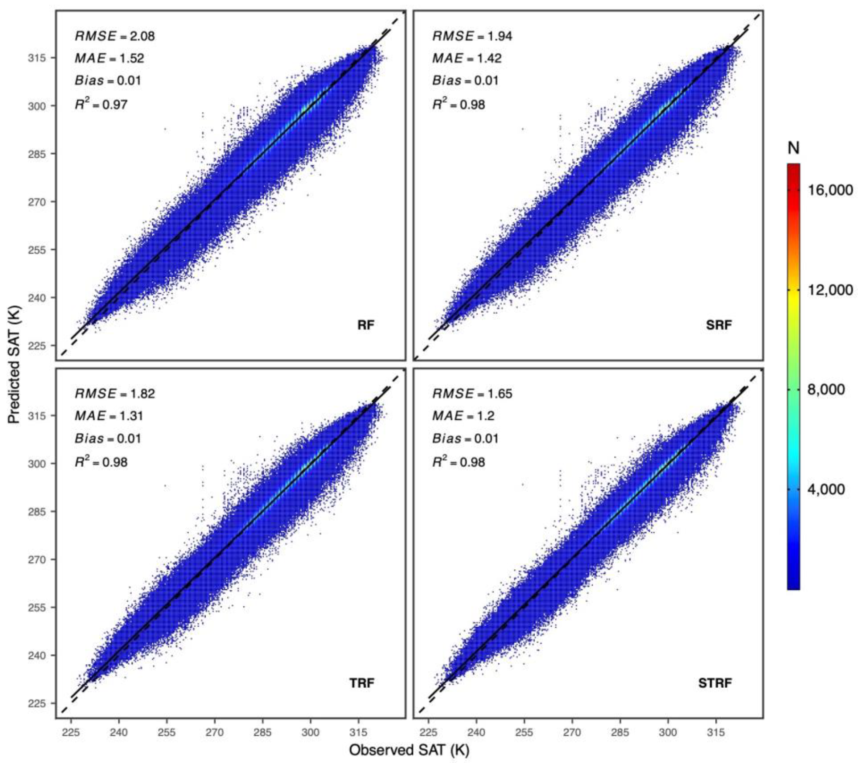
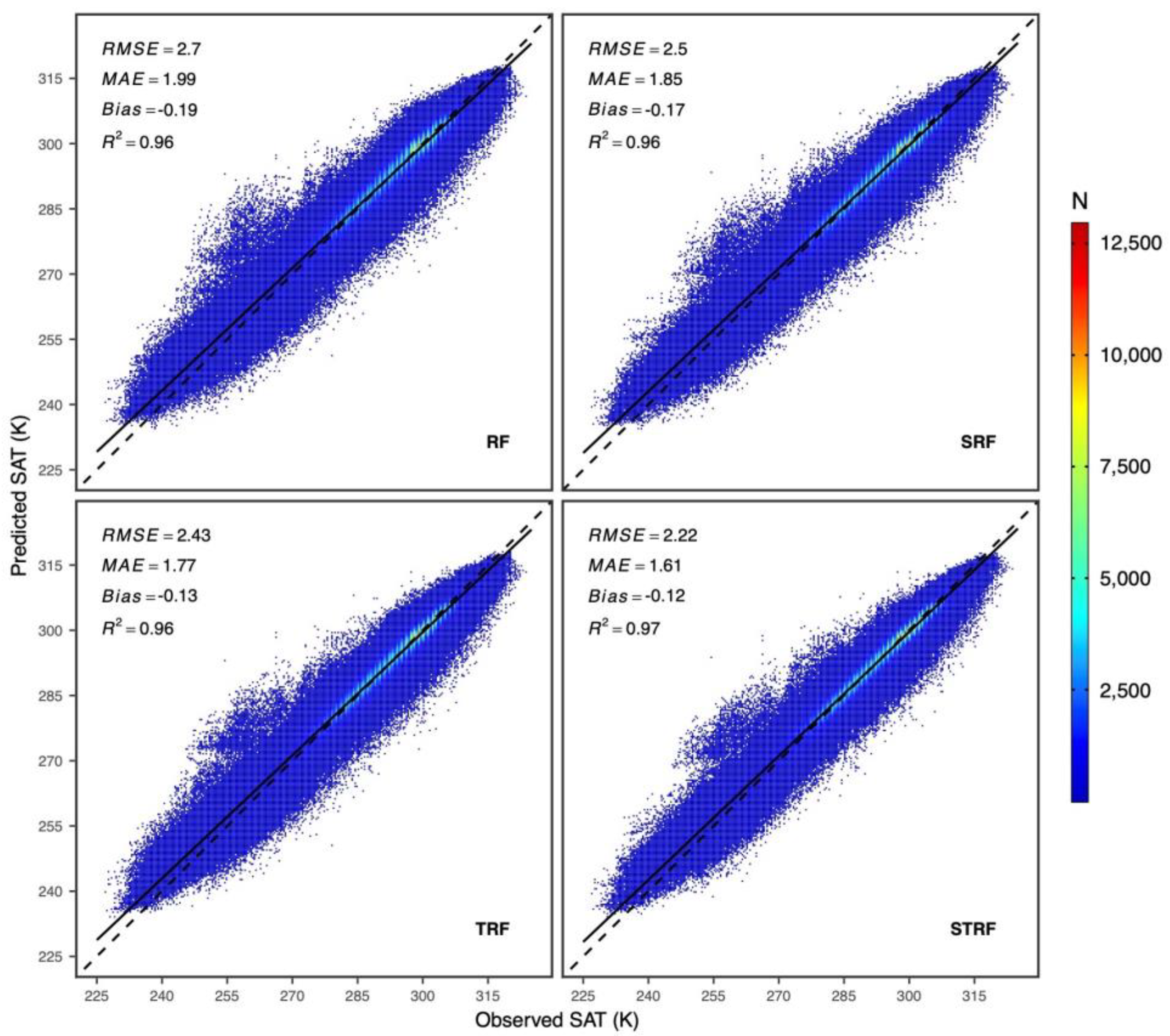
3.1. Overall Predictive Model Performance

The four specified hourly SAT estimation models were trained and validated using two types of 10-fold CV. For each of the four models, Figure 2 and Figure 3 compare the actual observed SAT and predicted SAT at ground sites using all validated data samples for sample-based and site-based CV, respectively. We observed that the incorporation of time-related and location-related variables into the estimation models can greatly increase the predictive performance for estimating hourly SAT, as seen in the two figures. Overall mean RMSE computed using all 10 folds of sample-based validated data samples is 2.08, 1.94, 1.82 and 1.65 K for RF, SRF, TRF and STRF, respectively. When cross-validated by sample-based CV, the SRF model that consider the location-related variables (longitude and latitude) and the TRF model that includes time-related variables (HOD and month), respectively, decrease the mean RMSE by about 0.14 and 0.26 K, compared to the baseline model RF. The decreases in the mean RMSE achieved by the two models are apparent as the relative decreasing rates of the two models are about 7% and 12.5% with respect to the mean RMSE of 2.08 K for the baseline model. Furthermore, the STRF model that considers both time- and location-related variables substantially increases the predictive performance of estimating hourly SAT with a decrease in RMSE by 0.43 K (a decreasing rate of 21%) relative to the baseline model RF.
Similarly, comparison of the four models using site-based CV, as shown in Figure 3, also indicates the increases in model performance due to the inclusion of time- and location-related variables in SAT hourly models. The baseline model RF has an overall RMSE of 2.7 K for site-based CV, while the mean RMSE of the other three models, SRF, TRF and STRF, are 2.5, 2.43, and 2.22 K, respectively. The best-performing estimation model STRF significantly reduces the predictive error by 0.48 K with a decreasing rate of 22%, compared to the baseline model RF. As spatial locations and distributional patterns of ground sites greatly influence statistical representation in the data samples, predictive errors (RMSE) of a model validated using site-based CV will be higher than the model validated using sample-based CV, which is revealed in Figure 2 and Figure 3.

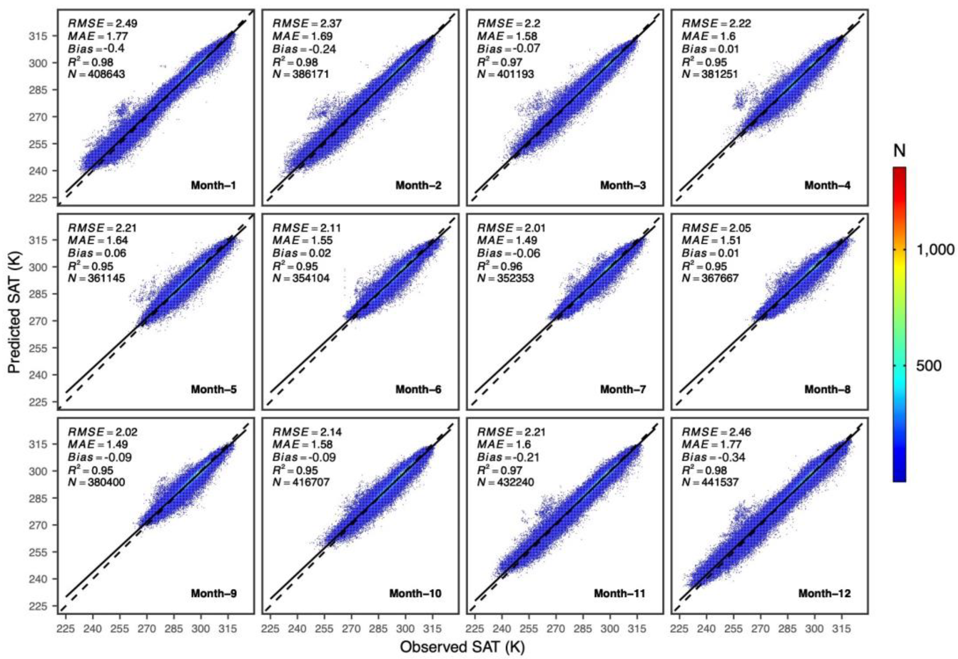
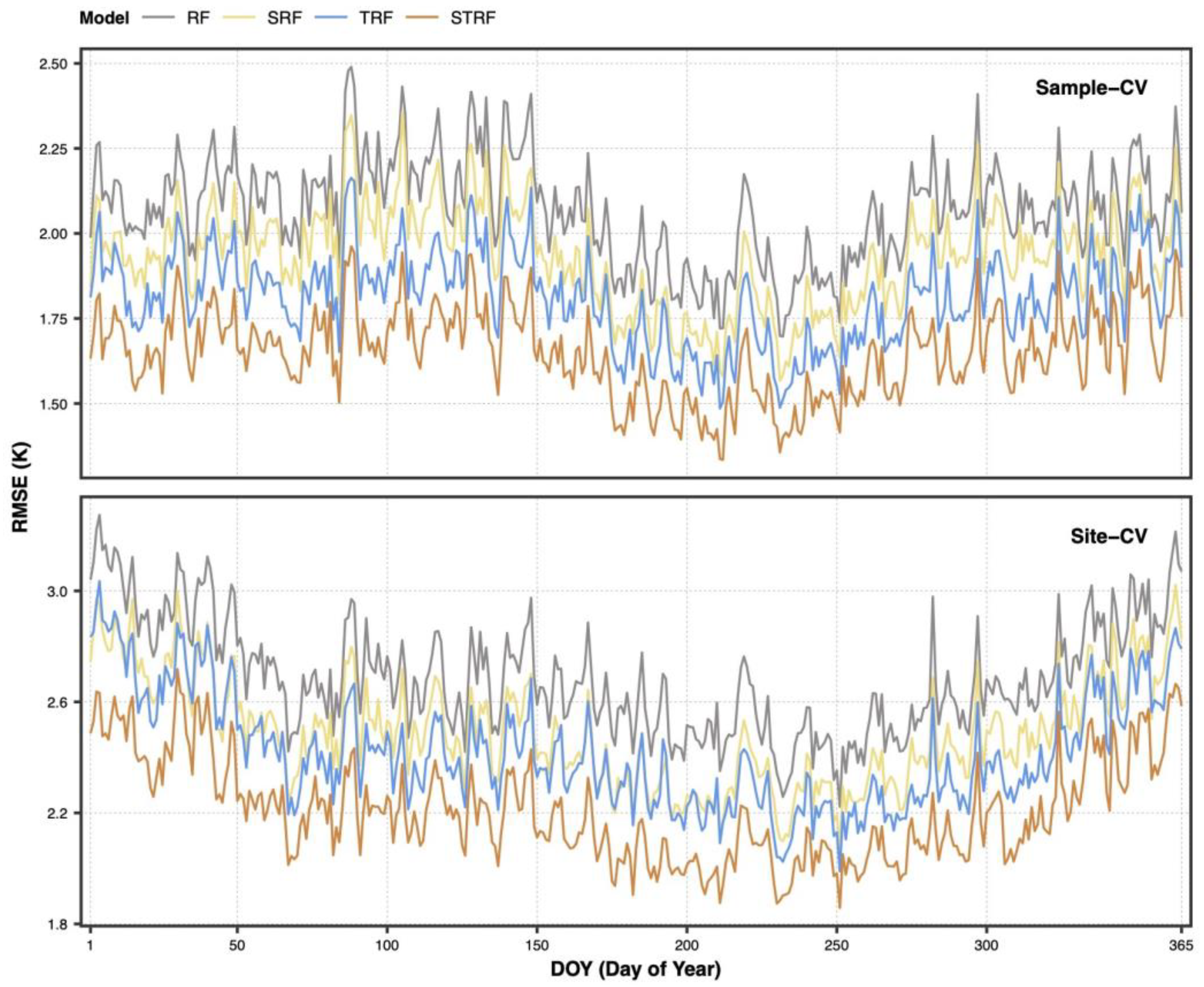
3.2. Temporal Variation in Model Performance

Site-based validated samples for the best-performing model STRF were used to compare the differences in model performance across months of the study period, which covers an entire year cycle (Figure 4). As seen from the figure, the mean RMSE across 12 months ranges from 2.01 to 2.49 K. STRF performs relatively better for summer months (July to September) with mean RMSE of about 2.0 K, while the model has higher predictive errors for winter months (December and January) with mean RMSE above 2.4 K. The difference in the mean RMSE across the months may be due to the temperature range and number of available samples used for model training and validation. In Figure 4, one can observe that number of data samples for summer months (indicated by the annotation N in the figure) is roughly 14% lower than that for winter months, and that the temperate ranges for summer months are considerably narrower than that for other months, especially for winter months, which is primarily because the study areas cover a large span of latitudes. The temperature contrasts between high latitudes and equatorial areas would be more distinct in winter months, and the models cross-validated using the data samples for all months will generally have lower RMSE for summer months. Thus, the different characteristics and the sizes of the data sample across the months lead to the temporal variation in model performance. The number of data samples differs across the months is due to the data gaps in the LST data product, which are primarily attributed to cloud contamination. Similar patterns are also revealed from Figure 5, which shows the mean RMSE on a daily basis for STRF using site-based validated samples. Thus, SAT estimation models should be cross-validated using data samples with varying temporal characteristics during long time periods, which could result in a more objective and conservative assessment of the predictive performance of SAT estimation models.

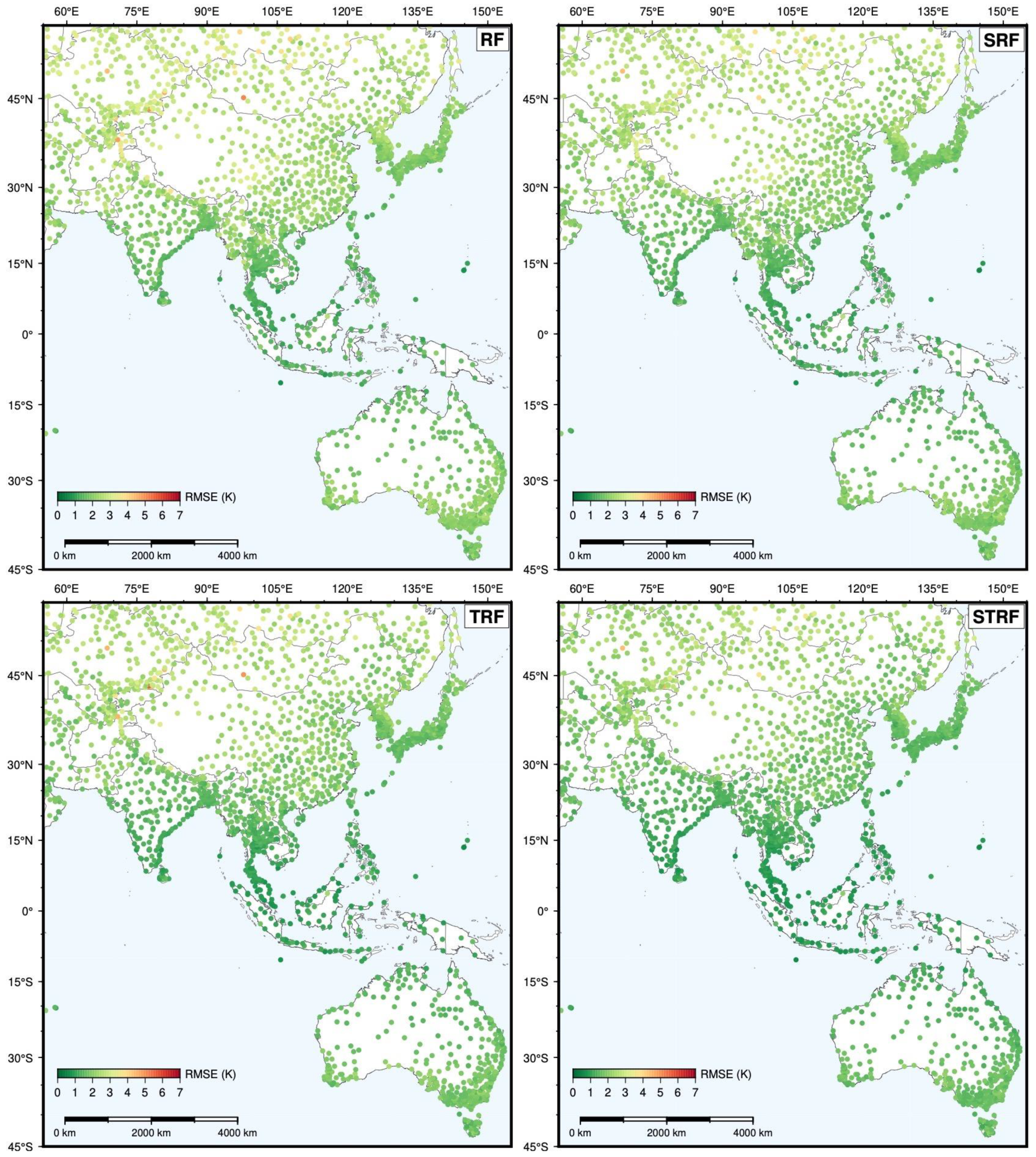
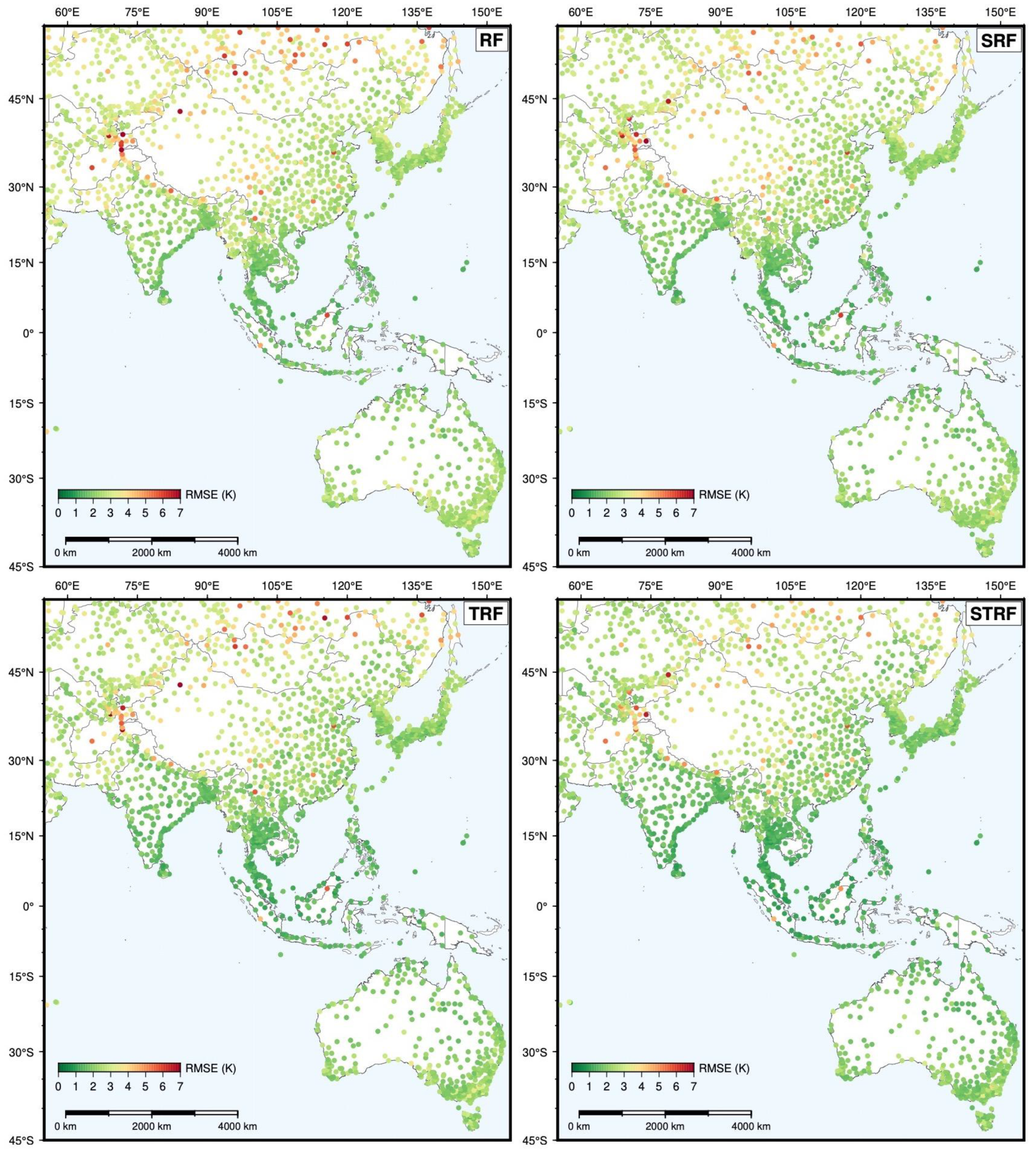
3.3. Predictive Performance across Sites

We computed the mean RMSE for each site across the study area using the cross-validated samples available at the site for the four models. Figure 6 and Figure 7 show the spatial distribution of site-specific mean RMSE of the four models for two types of cross-validation.
As shown in the two figures, the four models have relatively poorer performance for the sites at high latitudes (northern regions) than the sites at lower latitudes or regions around the Equator, which is more obvious for the four estimation models when validated by site-based CV (Figure 7). When using sample-based cross-validation, site-specific RMSE for the baseline model (RF) ranges from 2 to 3.5 K at most sites in northwestern areas (above 30°N), with RMSE for a few sites being more than 4 K. However, the higher RMSE errors for the sites in northwestern areas are apparently reduced by the estimation models considering time-related or location-related variables. The STRF model, which achieved the highest predictive performance in terms of overall RMSE, also performs better for the sites in northwestern areas with site-specific RMSE ranging from 1.0 to 2.5 K. Additionally, RMSE of the baseline model for the sites with extremely high errors (denoted as round dots colored with orange to red in Figure 6) decreases when using the STRF model. Compared to site-specific RMSE of the models cross-validated by sample-based CV, RMSE for the sites in northwestern areas, especially for the sites around the rim of the Tibetan Plateau and the sites in the Mongolian Plateau, is significantly higher than the sites at lower latitudes for the four models when using site-based CV (Figure 7). In addition to the high sensitivity of model performance to spatial distribution of sites used for model training, complex topographic features and local atmospheric conditions in the Tibetan Plateau and Mongolian Plateau may also lead to higher predictive errors for the sites in these regions when cross-validating the models in site-based CV. Site-specific RMSE of the baseline model for site-based CV in northwestern areas generally ranges from 3 to 4.5 K, with several sites having RMSE of more than 5 K. In contrast, site-specific RMSE of the STRF model for site-based CV has lower values in these areas, which primarily range from 2.5 to 3.5 K. It is worth noting that during a year, equatorial areas and lower latitudes experience narrow temperature ranges compared to broader temperature ranges in high-latitude areas, which may also influence the site-specific predictive errors.

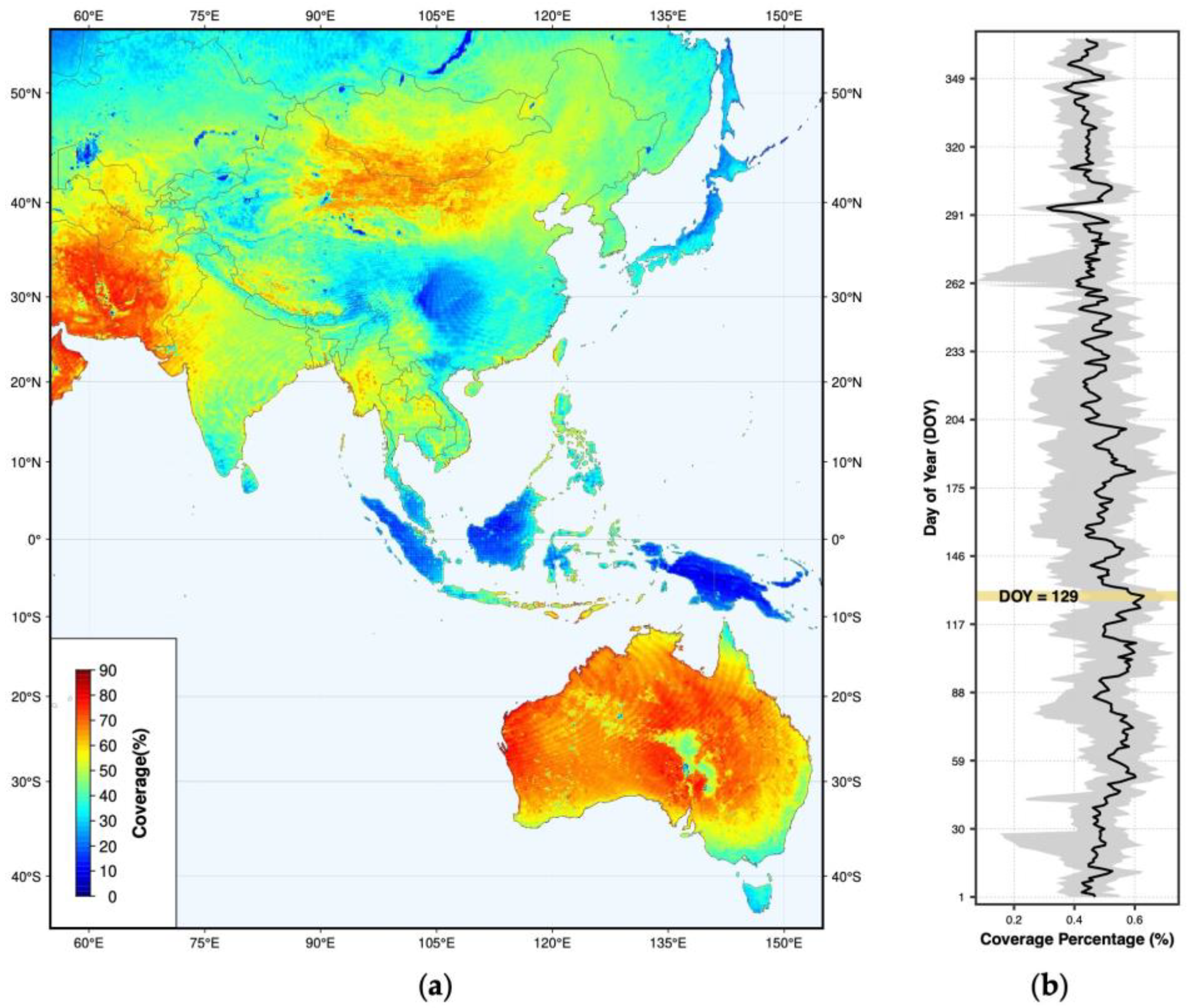
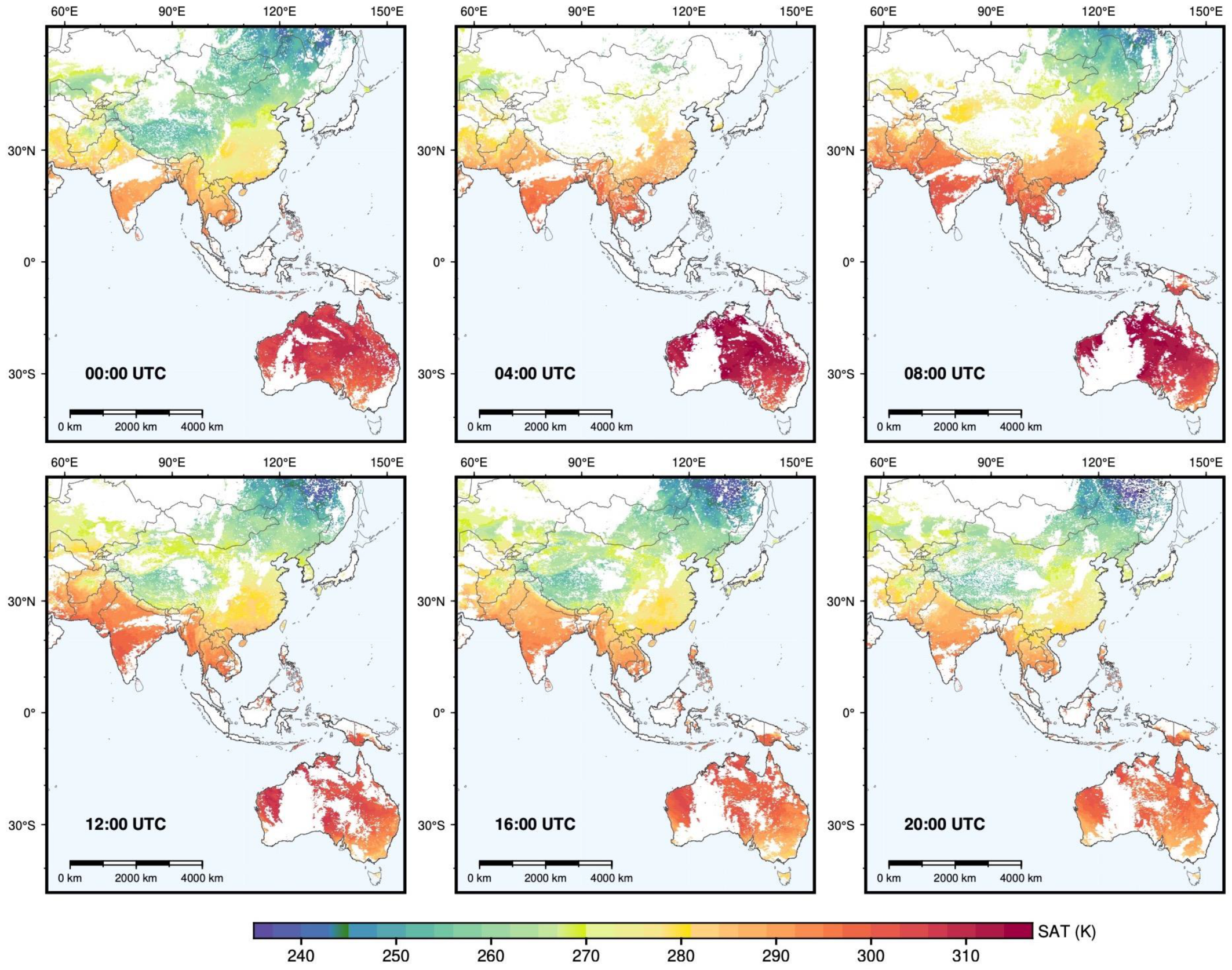
3.4. Coverage Analysis of Estimated SAT

The best-performing estimation model STRF was used to generate hourly maps of spatial continuous SAT over the study areas for each hour-point during the study period. As cloud coverage and heavy aerosol contamination conditions cause the missing values in the LST retrieval product, maps of estimated hourly SAT also suffer from the issue of missing values. To explore the spatial and temporal coverage of estimated hourly SAT, we computed daily coverage percentage and pixel-by-pixel annual coverage percentage, as shown in Figure 8.
Daily coverage percentage was computed as the mean of 24 coverage percentage values for each hour-point, which is the ratio of number of pixels with SAT estimates to total number of pixels in the study areas. Pixel-by-pixel annual coverage was computed for each pixel in the study areas and the percentage of the pixel is the ratio of the number of hours with SAT estimates to the total number of hours in a year. As can be seen from Figure 8, most parts of Australia and the Middle East have the distinctly higher coverage of SAT estimates with annual coverage percentage above 70%, while the equatorial areas, the Sichuan Basin and parts of Japan have lower coverage of SAT estimates with annual mean coverage below 30%. The spatial coverage of SAT estimates across different areas reflects the spatiotemporal coverage of clouds during the study period, which is controlled by atmospheric circulation and local atmospheric conditions. For example, the equatorial areas have high solar radiation and abundant warm water supply, facilitating cloud formation over these areas. Daily mean coverage of estimated SAT shown in Figure 8 is primarily between 42% and 58%, with the highest coverage occurring on the 129th day of a year cycle. Figure 9 shows the estimated SAT at six different hour-points for the day with the highest daily mean coverage. The pixels with missing values in the six maps shown in Figure 9 are denoted in white. We can observe that the estimates of SAT for the six hour-points over the equatorial land areas are nearly completely missing.

4. Discussion

4.1. Comparison with Previous Studies

In previous studies, substantial efforts have been made to estimate daily or monthly SAT using the LST derived from MODIS. Estimating high-temporal SAT, however, is only performed in very limited studies, and the studies are primarily based on the LST derived from the MSG geostationary satellites for small-scale areas. For examples, MSG SEVIRI LST has been used for sub-daily SAT estimation over small-scale areas by using the TVX or simple linear regression methods [30,31]. Zhou et al. [33] estimated hourly SAT for Israel using machine learning algorithms, which is also based on MSG LST. The study by Zhang and Du [27], for the first time, developed hourly SAT estimation models based on LST datasets derived from the GOES-R satellites by using learning algorithms for a large-scale area that contains most parts of North America. However, the hourly SAT estimation models developed in this study are for an even larger region that contains land areas of Asia and Oceania, and moreover, we are the first to apply the LST derived from China’s geostationary satellites FY-4 for SAT estimation. The hourly SAT estimation studies by Zhou et al. [33] and Zhang and Du [27] reported an overall RMSE of 0.9 K (sample-based cross-validation) and 1.9 K (site-based cross-validation), respectively. In this study, the best-performing model STRF achieved an overall RMSE of 1.65 for sample-based cross-validation and 2.22 K for site-based cross-validation. However, we should note that strictly comparing predictive performance of the models developed in different studies is meaningless in terms of only RMSE, as the RMSE computed from cross-validated samples is affected by many factors, such as selection of learning algorithms, parameter tuning, setting of hyperparameters and splitting of samples in cross-validation. In addition, data samples extracted from the areas with complex geographic settings or areas spanning large-scale geographic extents contain more spatiotemporal variability compared to small-scale areas, and thus, scales and selection of study areas also significantly affect the RMSE of cross-validated SAT estimation models.
Predictive performance of SAT estimation models is conventionally quantified by the statistical metrics computed using cross-validation approaches. All cross-validated samples can be used to calculate the mean RMSE for an overall assessment of model performance. However, the simple cross-validation (sample-based), in which samples are treated equally and are randomly split into different folds for training and validation, could result in serious overestimation of predictive performance for data samples with spatiotemporal structures in the field of spatial–temporal modeling [44,45]. Different types of cross-validation, including leave-location-out cross-validation (site-based), leave-time-out cross-validation (time-based) and leave-time-and-location-out cross-validation, are designed to account for the sensitivity of model performance to spatiotemporal structures in data samples [46]. In most recent years, there are many studies for SAT estimation that only used simple cross-validation approaches [10,25,33,47], which are inadequate for comprehensively evaluating predictive errors of SAT estimation models. Combination of the simple cross-validation and the approaches considering spatiotemporal characteristics, such as site-based cross-validation, should be ensured in SAT estimation studies [29,48,49]. As spatial patterns of ground sites significantly influence the training and validation of SAT models, site-based cross-validation generally yields higher predictive errors (RMSE) compared to simple sample-based cross-validation. For example, Zhang and Du [29] demonstrated that the overall mean RMSE of an ensemble of models based on different LST datasets for estimating daily SAT over China is 1.80 K for sample-based cross-validation and 2.06 K for site-based cross-validation. Similarly, Chen et al. [50] developed three daily SAT estimation models for mainland China and the mean RMSE of the three models assessed by sampled-based and site-based cross-validation is 1.41 and 1.79 K, respectively. In this study, predictive errors (RMSE) of the four specified hourly SAT estimation models for site-based cross-validation are all higher than that for sample-based cross-validation, with a difference of about 0.6 K. Therefore, a more conservative assessment of SAT estimation models could be ensured when using site-based cross-validation.
Analysis of predictive errors of the four hourly models across ground sites suggests that spatial configuration and density patterns of sites can influence model training. Sites in the areas with low coverage of stations and complex geographic settings, such as mountainous regions, generally have higher predictive errors, which are also confirmed in previous studies [49]. In this study, we observed that site-specific RMSE for the four hourly models is generally higher over the Tibetan Plateau and the Mongolian Plateau, which are covered with few stations. The studies for daily SAT over China [23,25,29,50] all showed higher predictive errors across the site in the Tibetan Plateau and the northwestern region of China due to the limited coverage of sites in these regions. Kilibarda et al. [21] used a spatiotemporal kriging model for estimating global daily SAT with the MODIS 8-day composite LST dataset and indicated that cross-validated RMSE for several sites in the areas with very low site density, such as the Tibetan Plateau and the western South America, can even approximate 6 K. Areas with a low density of meteorological stations are usually subject to complex geographic environments and variable atmospheric processes, and thus, samples from the very limited sites in the areas are severely under-represented, resulting in the poor predictive performance of SAT estimation models in these areas.
Although various learning methods have been applied to develop SAT estimation models in previous studies, the learning methods for their own sake have an absolute superiority. Performance of the SAT estimation models developed using different learning algorithms not only depends on the capability of the algorithms, but also relates to the factors that influence the RMSE computed from cross-validated samples, which are discussed above. In terms of the modeling task of hourly SAT estimation, models considering time-related and location-related variables generally achieve better performance, as indicated by the comparison of the four hourly models developed in this study. Given the characteristics of the modeling task of SAT estimation and the scales of complexity involved in the task, conventionally used ensemble learning algorithms, such as random forest and gradient boosting, are adequate for the task of modeling involved in SAT estimation. Random forest is widely used in SAT estimation studies due to its flexibility in modeling and insensitivity to overfitting. Recently, the studies for estimating hyperlocal SAT over urban areas using high-temporal LST derived from Landsat all adopted random forest [10,51,52]. The four hourly SAT estimation models developed in this study are based on random forest, and the models were not tuned exhaustively in cross-validation for pursing lower RMSE. Considering the large-scale study regions with broad geographic extents and diverse geographic settings, the reported RMSE for the four models using site-based cross-validation can be viewed as conservative indicators for the predictive performance of general models for estimating hourly SAT over large-scale areas, and the specifications of input variables for the four models have general implications for future studies on large-scale estimation of hourly SAT.

4.2. Implications for Future Studies

The differences in cross-validated RMSE between the four specified hourly SAT estimation models demonstrate the importance of considering the HOD variable in modeling hourly SAT, which is also confirmed in Zhang and Du [27]. Although LST derived from geostationary satellites provides the opportunity for estimating high-temporal SAT over large areas, geostationary LST have lower spatial resolutions compared to the LST retrieved from polar satellites, such as NASA’s Terra and Aqua, whose LST has been widely used for daily SAT estimation. For example, the operational LST products retrieved from GOES-R and FY-4A have a spatial resolution of 2 and 4 km, respectively. We should note that spatial resolutions of LST products are not equal to the nominal resolutions of the observations acquired by satellites, which depend on the size and shape of ground footprints of the observations. The footprints become more irregular and larger as the distance between the footprints and the nadir of satellites increases. Thus, estimates of SAT obtained from the models based on geostationary LST datasets, in fact, have spatially varying resolutions across the study area, and the inconsistency of spatial resolution is more severe for large-scale areas or areas far from the nadir of satellites. Models that integrate LST from polar-orbiting and geostationary satellites are a way for achieving estimates of SAT with spatially consistent resolutions across large-scale areas.
As clouds contaminate thermal infrared observations, LST datasets retrieved from TIR observations contain many missing pixels, resulting in the missing pixels in estimated SAT. To tackle the issue of missing estimates, gap-filling approaches that target on LST or estimated SAT have been explored in previous studies for obtaining seamless maps of SAT [19,53,54]. However, gap-filling approaches that infill missing pixels using the spatiotemporal information of their neighboring pixels can introduce large errors for missing pixels. Thus, gap-filling the missing estimates of SAT for the areas with high frequency and large blocks of cloud coverage, such as the equatorial areas, is nearly an impossible task because the pixels to be filled have no available neighboring pixels with estimates. As simulated air temperature in reanalysis datasets are spatially complete with high temporal resolutions but very low spatial resolutions, simulated SAT can be used with SAT estimation models for obtaining spatially complete estimates of SAT [55].

5. Conclusions

This study developed the models for estimating hourly SAT using the LST retrieved from FY-4A, which is a geostationary meteorological satellite in China’s Fengyun-4 mission. The hourly models were developed with a data sample from more than 3000 ground sites for a very large-scale study region, consisting of Asia and Oceania. In contrast to the baseline model RF specified with FY-4A LST and a set of auxiliary variables, three other models, including SRF, TRF and STRF, were also specified with the addition of time- and location-related variables. Overall predictive errors of the four models in terms of RMSE are about 1.65–2.08 K for sample-based cross-validation and 2.22–2.70 K for site-based cross-validation. The SRF and TRF models, which, respectively, consider time and location variables, reduce predictive errors by about 0.15–0.20 K and 0.26–0.27 K with respect to the baseline model. Temporal variation and site-specific patterns of predictive errors across the four models were analyzed, and their differences across the models indicate the importance of incorporating time and location information into SAT estimation models. Different types of cross-validation approaches have great impacts on the training and assessment of SAT estimation models. Spatial configuration and density of the sites used in model training greatly influence the representativeness and spatiotemporal variability of the data samples extracted at the sites, and thus site-based cross-validation usually produces larger RMSE compared to simple sample-based cross-validation. Overall RMSE of the four models in this study for the site-based cross-validation is about 0.5 K higher than that for sample-based cross-validation, and could be used as conservative indicators for assessing the predictive performance of general hourly SAT estimation models. Random forest is insensitive to model overfitting and the four hourly SAT estimation models specified in this study were not tuned exhaustively in pursing lower errors. In addition, the four models were developed and comprehensively cross-validated for a very large-scale area with diverse geographic settings. Therefore, the four hourly models have general implications for future studies on large-scale estimation of hourly SAT based on geostationary LST datasets.

Author Contributions

Conceptualization, Z.Z.; methodology, Z.Z. and Y.L.; software, Z.Z.; validation, Z.Z., Y.L. and G.Z.; formal analysis, Z.Z. and C.L.; investigation, Z.Z. and Y.L.; resources, Z.Z., Y.L. and G.Z.; data curation, Z.Z.; writing—original draft preparation, Z.Z.; writing—review and editing, Z.Z.; visualization, Z.Z. and G.Z.; supervision, Z.Z.; project administration, Z.Z.; funding acquisition, Z.Z. All authors have read and agreed to the published version of the manuscript.

Funding

This research was funded by the Startup Foundation for Introducing Talent of NUIST, grant number 2022r040.

Data Availability Statement

Datasets used in this study were obtained from publicly available data sources, which are archived and maintained by the Earth observation data centers, including NASA LP DAAC, NOAA NCDC, Copernicus S3C CDC, and CMA NSMC. Section 2.2 can be referred to for detailed information on the datasets and their related data sources.

Conflicts of Interest

The authors declare no conflict of interest.

References

  1. Hansen, J.; Sato, M.; Ruedy, R.; Lo, K.; Lea, D.W.; Medina-Elizade, M. Global Temperature Change. Proc. Natl. Acad. Sci. USA 2006, 103, 14288–14293. [Google Scholar] [CrossRef] [PubMed] [Green Version]
  2. Menne, M.J.; Durre, I.; Vose, R.S.; Gleason, B.E.; Houston, T.G. An Overview of the Global Historical Climatology Network-Daily Database. J. Atmos. Ocean. Technol. 2012, 29, 897–910. [Google Scholar] [CrossRef]
  3. Menne, M.J.; Williams, C.N.; Gleason, B.E.; Rennie, J.J.; Lawrimore, J.H. The Global Historical Climatology Network Monthly Temperature Dataset, Version 4. J. Clim. 2018, 31, 9835–9854. [Google Scholar] [CrossRef]
  4. Pichierri, M.; Bonafoni, S.; Biondi, R. Satellite Air Temperature Estimation for Monitoring the Canopy Layer Heat Island of Milan. Remote Sens. Environ. 2012, 127, 130–138. [Google Scholar] [CrossRef]
  5. Schuster, C.; Burkart, K.; Lakes, T. Heat Mortality in Berlin—Spatial Variability at the Neighborhood Scale. Urban Clim. 2014, 10, 134–147. [Google Scholar] [CrossRef]
  6. Shamir, E.; Georgakakos, K.P. MODIS Land Surface Temperature as an Index of Surface Air Temperature for Operational Snowpack Estimation. Remote Sens. Environ. 2014, 152, 83–98. [Google Scholar] [CrossRef]
  7. Lutz, A.F.; Immerzeel, W.W.; Shrestha, A.B.; Bierkens, M.F.P. Consistent Increase in High Asia’s Runoff Due to Increasing Glacier Melt and Precipitation. Nat. Clim. Chang. 2014, 4, 587–592. [Google Scholar] [CrossRef] [Green Version]
  8. Vogt, J.R.V.; Viau, A.A.; Paquet, F. Mapping Regional Air Temperature Fields Using Satellite-Derived Surface Skin Temperatures. Int. J. Climatol. 1997, 17, 1559–1579. [Google Scholar] [CrossRef]
  9. Vancutsem, C.; Ceccato, P.; Dinku, T.; Connor, S.J. Evaluation of MODIS Land Surface Temperature Data to Estimate Air Temperature in Different Ecosystems over Africa. Remote Sens. Environ. 2010, 114, 449–465. [Google Scholar] [CrossRef]
  10. Venter, Z.S.; Brousse, O.; Esau, I.; Meier, F. Hyperlocal Mapping of Urban Air Temperature Using Remote Sensing and Crowdsourced Weather Data. Remote Sens. Environ. 2020, 242, 111791. [Google Scholar] [CrossRef]
  11. Zhang, Z.; Du, Q. A Bayesian Kriging Regression Method to Estimate Air Temperature Using Remote Sensing Data. Remote Sens. 2019, 11, 767. [Google Scholar] [CrossRef] [Green Version]
  12. Meyer, H.; Schmidt, J.; Detsch, F.; Nauss, T. Hourly Gridded Air Temperatures of South Africa Derived from MSG SEVIRI. Int. J. Appl. Earth Obs. Geoinf. 2019, 78, 261–267. [Google Scholar] [CrossRef]
  13. Zhu, W.; Lű, A.; Jia, S. Estimation of Daily Maximum and Minimum Air Temperature Using MODIS Land Surface Temperature Products. Remote Sens. Environ. 2013, 130, 62–73. [Google Scholar] [CrossRef]
  14. Prihodko, L.; Goward, S.N. Estimation of Air Temperature from Remotely Sensed Surface Observations. Remote Sens. Environ. 1997, 60, 335–346. [Google Scholar] [CrossRef]
  15. Czajkowski, K.; Goward, S.; Stadler, S.; Walz, A. Thermal Remote Sensing of Near Surface Environmental Variables: Application Over the Oklahoma Mesonet. Prof. Geogr. 2000, 52, 345–357. [Google Scholar] [CrossRef]
  16. Zakšek, K.; Schroedter-Homscheidt, M. Parameterization of Air Temperature in High Temporal and Spatial Resolution from a Combination of the SEVIRI and MODIS Instruments. ISPRS J. Photogramm. Remote Sens. 2009, 64, 414–421. [Google Scholar] [CrossRef]
  17. Sun, Y.; Wang, J.; Zhang, R.; Gillies, R.R.; Xue, Y.; Bo, Y. Air Temperature Retrieval from Remote Sensing Data Based on Thermodynamics. Theor. Appl. Climatol. 2005, 80, 37–48. [Google Scholar] [CrossRef]
  18. Florio, E.N.; Lele, S.R.; Chi Chang, Y.; Sterner, R.; Glass, G.E. Integrating AVHRR Satellite Data and NOAA Ground Observations to Predict Surface Air Temperature: A Statistical Approach. Int. J. Remote Sens. 2004, 25, 2979–2994. [Google Scholar] [CrossRef]
  19. Kloog, I.; Nordio, F.; Coull, B.A.; Schwartz, J. Predicting Spatiotemporal Mean Air Temperature Using MODIS Satellite Surface Temperature Measurements across the Northeastern USA. Remote Sens. Environ. 2014, 150, 132–139. [Google Scholar] [CrossRef]
  20. Hengl, T.; Heuvelink, G.B.M.; Tadic, M.P.; Pebesma, E.J. Spatio-Temporal Prediction of Daily Temperatures Using Time-Series of MODIS LST Images. Theor. Appl. Climatol. 2012, 107, 265–277. [Google Scholar] [CrossRef] [Green Version]
  21. Kilibarda, M.; Hengl, T.; Heuvelink, G.B.M.; Gräler, B.; Pebesma, E.; Perčec Tadić, M.; Bajat, B. Spatio-temporal Interpolation of Daily Temperatures for Global Land Areas at 1 Km Resolution. J. Geophys. Res. Atmos. 2014, 119, 2294–2313. [Google Scholar] [CrossRef] [Green Version]
  22. Noi, P.T.; Degener, J.; Kappas, M. Comparison of Multiple Linear Regression, Cubist Regression, and Random Forest Algorithms to Estimate Daily Air Surface Temperature from Dynamic Combinations of MODIS LST Data. Remote Sens. 2017, 9, 398. [Google Scholar] [CrossRef] [Green Version]
  23. Rao, Y.; Liang, S.; Wang, D.; Yu, Y.; Song, Z.; Zhou, Y.; Shen, M.; Xu, B. Estimating Daily Average Surface Air Temperature Using Satellite Land Surface Temperature and Top-of-Atmosphere Radiation Products over the Tibetan Plateau. Remote Sens. Environ. 2019, 234, 111462. [Google Scholar] [CrossRef]
  24. Yoo, C.; Im, J.; Park, S.; Quackenbush, L.J. Estimation of Daily Maximum and Minimum Air Temperatures in Urban Landscapes Using MODIS Time Series Satellite Data. ISPRS J. Photogramm. Remote Sens. 2018, 137, 149–162. [Google Scholar] [CrossRef]
  25. Shen, H.; Jiang, Y.; Li, T.; Cheng, Q.; Zeng, C.; Zhang, L. Deep Learning-Based Air Temperature Mapping by Fusing Remote Sensing, Station, Simulation and Socioeconomic Data. Remote Sens. Environ. 2020, 240, 111692. [Google Scholar] [CrossRef] [Green Version]
  26. LeCun, Y.; Bengio, Y.; Hinton, G. Deep Learning. Nature 2015, 521, 436–444. [Google Scholar] [CrossRef]
  27. Zhang, Z.; Du, Q. Hourly Mapping of Surface Air Temperature by Blending Geostationary Datasets from the Two-Satellite System of GOES-R Series. ISPRS J. Photogramm. Remote Sens. 2022, 183, 111–128. [Google Scholar] [CrossRef]
  28. Alqasemi, A.S.; Hereher, M.E.; Al-Quraishi, A.M.F.; Saibi, H.; Aldahan, A.; Abuelgasim, A. Retrieval of Monthly Maximum and Minimum Air Temperature Using MODIS Aqua Land Surface Temperature Data over the United Arab Emirates. Geocarto Int. 2022, 37, 2996–3013. [Google Scholar] [CrossRef]
  29. Zhang, Z.; Du, Q. Merging Framework for Estimating Daily Surface Air Temperature by Integrating Observations from Multiple Polar-Orbiting Satellites. Sci. Total Environ. 2022, 812, 152538. [Google Scholar] [CrossRef]
  30. Stisen, S.; Sandholt, I.; Nørgaard, A.; Fensholt, R.; Eklundh, L. Estimation of Diurnal Air Temperature Using MSG SEVIRI Data in West Africa. Remote Sens. Environ. 2007, 110, 262–274. [Google Scholar] [CrossRef]
  31. Nieto, H.; Sandholt, I.; Aguado, I.; Chuvieco, E.; Stisen, S. Air Temperature Estimation with MSG-SEVIRI Data: Calibration and Validation of the TVX Algorithm for the Iberian Peninsula. Remote Sens. Environ. 2011, 115, 107–116. [Google Scholar] [CrossRef] [Green Version]
  32. Lazzarini, M.; Marpu, P.R.; Eissa, Y.; Ghedira, H. Toward a Near Real-Time Product of Air Temperature Maps from Satellite Data and In Situ Measurements in Arid Environments. IEEE J. Sel. Top. Appl. Earth Obs. Remote Sens. 2014, 7, 3093–3104. [Google Scholar] [CrossRef]
  33. Zhou, B.; Erell, E.; Hough, I.; Shtein, A.; Just, A.C.; Novack, V.; Rosenblatt, J.; Kloog, I. Estimation of Hourly near Surface Air Temperature Across Israel Using an Ensemble Model. Remote Sens. 2020, 12, 1741. [Google Scholar] [CrossRef]
  34. Yang, J.; Zhang, Z.; Wei, C.; Lu, F.; Guo, Q. Introducing the New Generation of Chinese Geostationary Weather Satellites, Fengyun-4. Bull. Am. Meteorol. Soc. 2017, 98, 1637–1658. [Google Scholar] [CrossRef]
  35. Smith, A.; Lott, N.; Vose, R. The Integrated Surface Database: Recent Developments and Partnerships. Bull. Am. Meteorol. Soc. 2011, 92, 704–708. [Google Scholar] [CrossRef] [Green Version]
  36. Xian, D.; Zhang, P.; Gao, L.; Sun, R.; Zhang, H.; Jia, X. Fengyun Meteorological Satellite Products for Earth System Science Applications. Adv. Atmos. Sci. 2021, 38, 1267–1284. [Google Scholar] [CrossRef]
  37. Min, M.; Wu, C.; Li, C.; Liu, H.; Xu, N.; Wu, X.; Chen, L.; Wang, F.; Sun, F.; Qin, D.; et al. Developing the Science Product Algorithm Testbed for Chinese Next-Generation Geostationary Meteorological Satellites: Fengyun-4 Series. J. Meteorol. Res. 2017, 31, 708–719. [Google Scholar] [CrossRef]
  38. Wan, Z.; Dozier, J. A Generalized Split-Window Algorithm for Retrieving Land-Surface Temperature from Space. IEEE Trans. Geosci. Remote Sens. 1996, 34, 892–905. [Google Scholar]
  39. Yu, Y.; Tarpley, D.; Privette, J.L.; Goldberg, M.D.; Rama Varma Raja, M.K.; Vinnikov, K.Y.; Xu, H. Developing Algorithm for Operational GOES-R Land Surface Temperature Product. IEEE Trans. Geosci. Remote Sens. 2009, 47, 936–951. [Google Scholar]
  40. Trigo, I.F.; Ermida, S.L.; Martins, J.P.; Gouveia, C.M.; Göttsche, F.-M.; Freitas, S.C. Validation and Consistency Assessment of Land Surface Temperature from Geostationary and Polar Orbit Platforms: SEVIRI/MSG and AVHRR/Metop. ISPRS J. Photogramm. Remote Sens. 2021, 175, 282–297. [Google Scholar] [CrossRef]
  41. Fan, J.; Han, Q.; Wang, S.; Liu, H.; Chen, L.; Tan, S.; Song, H.; Li, W. Evaluation of Fengyun-4A Detection Accuracy: A Case Study of the Land Surface Temperature Product for Hunan Province, Central China. Atmosphere 2022, 13, 1953. [Google Scholar] [CrossRef]
  42. Li, R.; Li, H.; Bian, Z.; Cao, B.; Du, Y.; Sun, L.; Liu, Q. High Temporal Resolution Land Surface Temperature Retrieval from Global Geostationary Satellite Data. In Proceedings of the IEEE International Geoscience and Remote Sensing Symposium, Yokohama, Japan, 28 July–2 August 2019. [Google Scholar]
  43. Meng, Y.; Zhou, J.; Ma, J.; Long, Z. Investigation and Validation of The Chinese Fengyun-4a Land Surface Temperature Products In The Heihe River Basin. In Proceedings of the IEEE International Geoscience and Remote Sensing Symposium IGARSS, Brussels, Belgium, 11–16 July 2021. [Google Scholar]
  44. Roberts, D.R.; Bahn, V.; Ciuti, S.; Boyce, M.S.; Elith, J.; Guillera-Arroita, G.; Hauenstein, S.; Lahoz-Monfort, J.J.; Schröder, B.; Thuiller, W.; et al. Cross-Validation Strategies for Data with Temporal, Spatial, Hierarchical, or Phylogenetic Structure. Ecography 2017, 40, 913–929. [Google Scholar] [CrossRef] [Green Version]
  45. Wadoux, A.M.J.-C.; Heuvelink, G.B.M.; de Bruin, S.; Brus, D.J. Spatial Cross-Validation Is Not the Right Way to Evaluate Map Accuracy. Ecol. Modell. 2021, 457, 109692. [Google Scholar] [CrossRef]
  46. Meyer, H.; Reudenbach, C.; Wöllauer, S.; Nauss, T. Importance of Spatial Predictor Variable Selection in Machine Learning Applications—Moving from Data Reproduction to Spatial Prediction. Ecol. Modell. 2019, 411, 108815. [Google Scholar] [CrossRef] [Green Version]
  47. Gutiérrez-Avila, I.; Arfer, K.B.; Wong, S.; Rush, J.; Kloog, I.; Just, A.C. A Spatiotemporal Reconstruction of Daily Ambient Temperature Using Satellite Data in the Megalopolis of Central Mexico from 2003 to 2019. Int. J. Climatol. 2021, 41, 4095–4111. [Google Scholar] [CrossRef]
  48. Zeng, L.; Hu, Y.; Wang, R.; Zhang, X.; Peng, G.; Huang, Z.; Zhou, G.; Xiang, D.; Meng, R.; Wu, W.; et al. 8-Day and Daily Maximum and Minimum Air Temperature Estimation via Machine Learning Method on a Climate Zone to Global Scale. Remote Sens. 2021, 13, 2355. [Google Scholar] [CrossRef]
  49. Bahari, N.I.S.; Muharam, F.M.; Zulkafli, Z.; Mazlan, N.; Husin, N.A. Modified Linear Scaling and Quantile Mapping Mean Bias Correction of MODIS Land Surface Temperature for Surface Air Temperature Estimation for the Lowland Areas of Peninsular Malaysia. Remote Sens. 2021, 13, 2589. [Google Scholar] [CrossRef]
  50. Chen, Y.; Liang, S.; Ma, H.; Li, B.; He, T.; Wang, Q. An All-Sky 1 Km Daily Land Surface Air Temperature Product over Mainland China for 2003–2019 from MODIS and Ancillary Data. Earth Syst. Sci. Data 2021, 13, 4241–4261. [Google Scholar] [CrossRef]
  51. Zumwald, M.; Knüsel, B.; Bresch, D.N.; Knutti, R. Mapping Urban Temperature Using Crowd-Sensing Data and Machine Learning. Urban Clim. 2021, 35, 100739. [Google Scholar] [CrossRef]
  52. Cho, D.; Yoo, C.; Im, J.; Lee, Y.; Lee, J. Improvement of Spatial Interpolation Accuracy of Daily Maximum Air Temperature in Urban Areas Using a Stacking Ensemble Technique. GIsci. Remote Sens. 2020, 57, 633–649. [Google Scholar] [CrossRef]
  53. Zhang, M.; Wang, B.; Cleverly, J.; Liu, D.L.; Feng, P.; Zhang, H.; Huete, A.; Yang, X.; Yu, Q. Creating New Near-Surface Air Temperature Datasets to Understand Elevation-Dependent Warming in the Tibetan Plateau. Remote Sens. 2020, 12, 1722. [Google Scholar] [CrossRef]
  54. Li, X.; Zhou, Y.; Asrar, G.R.; Zhu, Z. Developing a 1 Km Resolution Daily Air Temperature Dataset for Urban and Surrounding Areas in the Conterminous United States. Remote Sens. Environ. 2018, 215, 74–84. [Google Scholar] [CrossRef]
  55. Zhang, H.; Immerzeel, W.W.; Zhang, F.; de Kok, R.J.; Gorrie, S.J.; Ye, M. Creating 1-Km Long-Term (1980–2014) Daily Average Air Temperatures over the Tibetan Plateau by Integrating Eight Types of Reanalysis and Land Data Assimilation Products Downscaled with MODIS-Estimated Temperature Lapse Rates Based on Machine Learning. Int. J. Appl. Earth Obs. Geoinf. 2021, 97, 102295. [Google Scholar] [CrossRef]
Figure 1. Map of the study areas overlaid with the ground meteorological sites used for developing SAT estimation models. The inset map on the lower left shows the full-disc observation area of the FY-4A geostationary satellite, which is delimited by the black line, and the spatial extent of study areas is denoted by the red line.
Remotesensing 15 01753 g001
Figure 2. Overall agreement between observed SAT and predicted SAT using sample-based cross-validation for the four hourly SAT estimation models (RF, SRF, TRF, STRF).
Remotesensing 15 01753 g002
Figure 3. Overall agreement between observed SAT and predicted SAT using site-based cross-validation for the four hourly SAT estimation models (RF, SRF, TRF, STRF).
Remotesensing 15 01753 g003
Figure 4. Comparison of mean predictive performance (RMSE) of the STRF model across the months for site-based CV.
Remotesensing 15 01753 g004
Figure 5. Daily variation in predictive performance (RMSE) of the STRF model for site-based CV.
Remotesensing 15 01753 g005
Figure 6. Spatial distribution of site-specific mean RMSE across the study area for the four hourly estimation models using sample-based cross-validation.
Remotesensing 15 01753 g006
Figure 7. Spatial distribution of site-specific mean RMSE across the study area for the four hourly estimation models using site-based cross-validation.
Remotesensing 15 01753 g007
Figure 8. Spatial coverage of hourly maps of SAT estimated using the STRF model: (a) annual coverage percentage on a pixel-by-pixel basis; (b) daily mean coverage percentage of the estimated maps at 24 h points of a day (denoted by the black line) with the gray ribbon indicating the lowest and highest coverage of the 24 maps of hourly SAT.
Remotesensing 15 01753 g008
Figure 9. Examples of estimated SAT for six hour-points of the day with the highest daily coverage throughout the study period.
Remotesensing 15 01753 g009
Table 1. Data sources from which the input variables for SAT estimation models were extracted.
DatasetVariable TypeResolutionSource 1
ISDground site observationshourly, point-scaleNOAA NCDC
FY-4A LSTland surface temperaturehourly, 4 kmCMA NSMC
MOD13C1vegetation indices16 day, 0.05°NASA LP DAAC
MCD12C1land cover typesyearly, 0.05°NASA LP DAAC
ERA5atmospheric reanalysishourly, 0.25°C3S CDS
GMTED2010global digital elevationstatic, ~1 km USGS
1 The datasets used in this study can be accessed from: NOAA National Climatic Data Center (NCDC, https://www.ncdc.noaa.gov/isd, accessed on 12 June 2022), CMA NSMC (China Meteorological Administration, National Satellite Meteorological Center, http://satellite.nsmc.org.cn, accessed on 23 September 2022), LP DAAC (The Land Processes Distributed Active Archive Center, https://lpdaac.usgs.gov, accessed on 23 September 2022), C3S CDS (Copernicus Climate Change Service, Copernicus Climate Data Store, https://cds.climate.copernicus.eu, accessed on 2 July 2022), and USGS GMTED2010 (https://www.usgs.gov/coastal-changes-and-impacts/gmted2010, accessed on 5 July 2022).
Table 2. Input variables specified for the four hourly SAT estimation models.
ModelInput Variables 1
RFbaseline inputs = {LST, NDVI, ELEV, SLP, LCPWAT, LCPURB, LCPHF, TCW, BLH, SSR}
SRF{baseline inputs} + {LON + LAT}
TRF{baseline inputs} + {HOD + MON}
STRF{baseline inputs} + {HOD + MON + LON + LAT}
1 ELEV and SLP represent topographic elevations and slope, respectively. LCPWAT, LCPURB and LCPHF are the percentages of the areas covered by water, urban and vegetation, respectively, and the three variables are extracted from the MCD12C1 dataset. Total column water (TCW), boundary layer height (BLH) and surface solar radiation (SSR) are simulated atmospheric state variables that are extracted from the ERA5 reanalysis dataset. LON and LAT are location variables for longitude and latitude. Time-related variables include HOD (hour of day) and MON (month of a year).
Disclaimer/Publisher’s Note: The statements, opinions and data contained in all publications are solely those of the individual author(s) and contributor(s) and not of MDPI and/or the editor(s). MDPI and/or the editor(s) disclaim responsibility for any injury to people or property resulting from any ideas, methods, instructions or products referred to in the content.

