

Comparing Global Sentinel-2 Land Cover Maps for Regional Species Distribution Modeling
 , , and
Abstract
:
1. Introduction
2. Methods
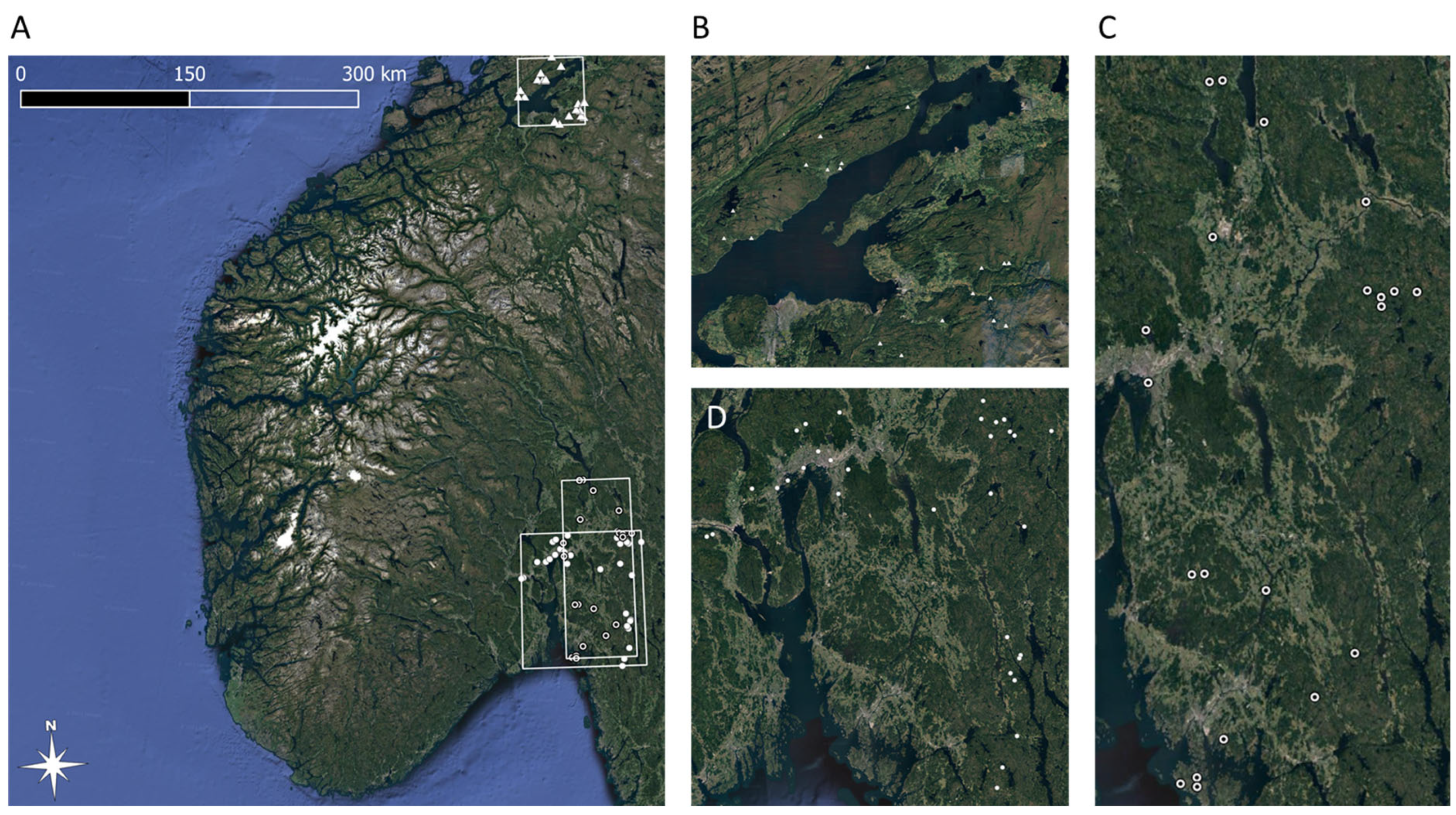
2.1. Solitary Bee Surveys
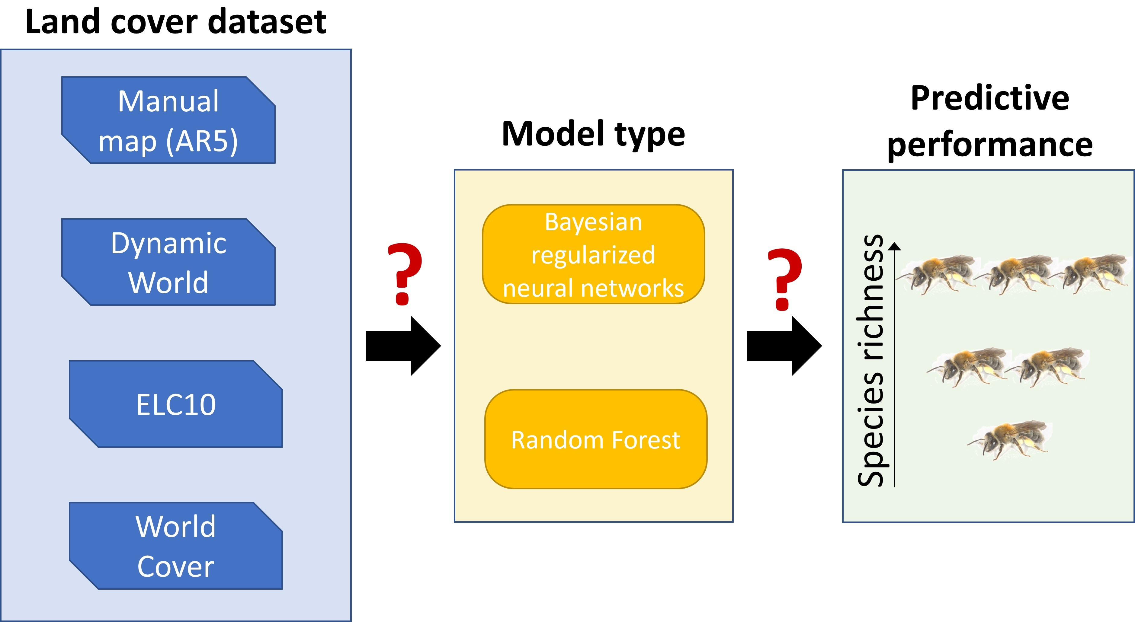
2.2. Land Cover Maps
2.3. Modeling
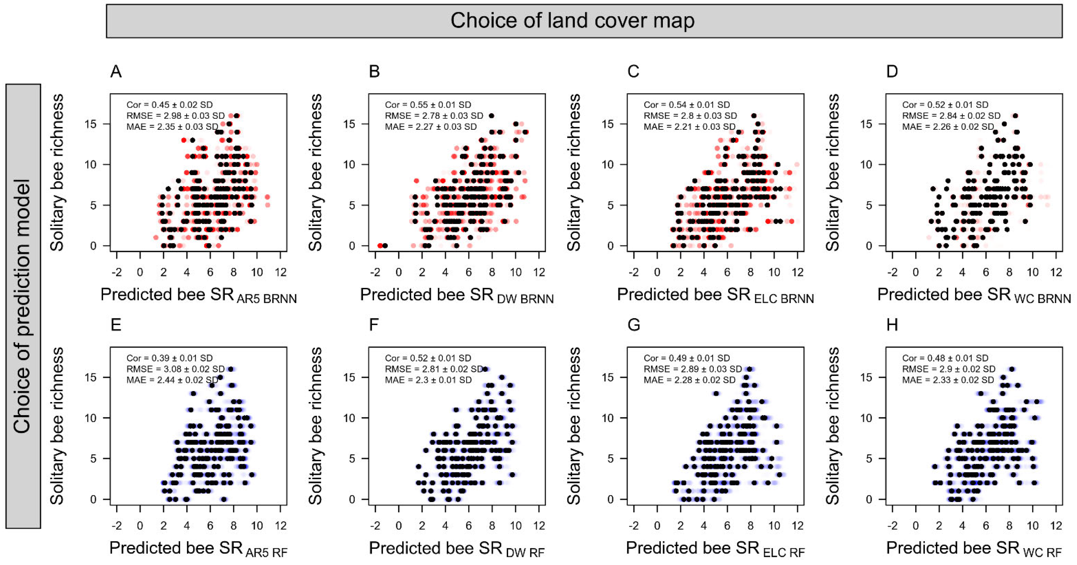
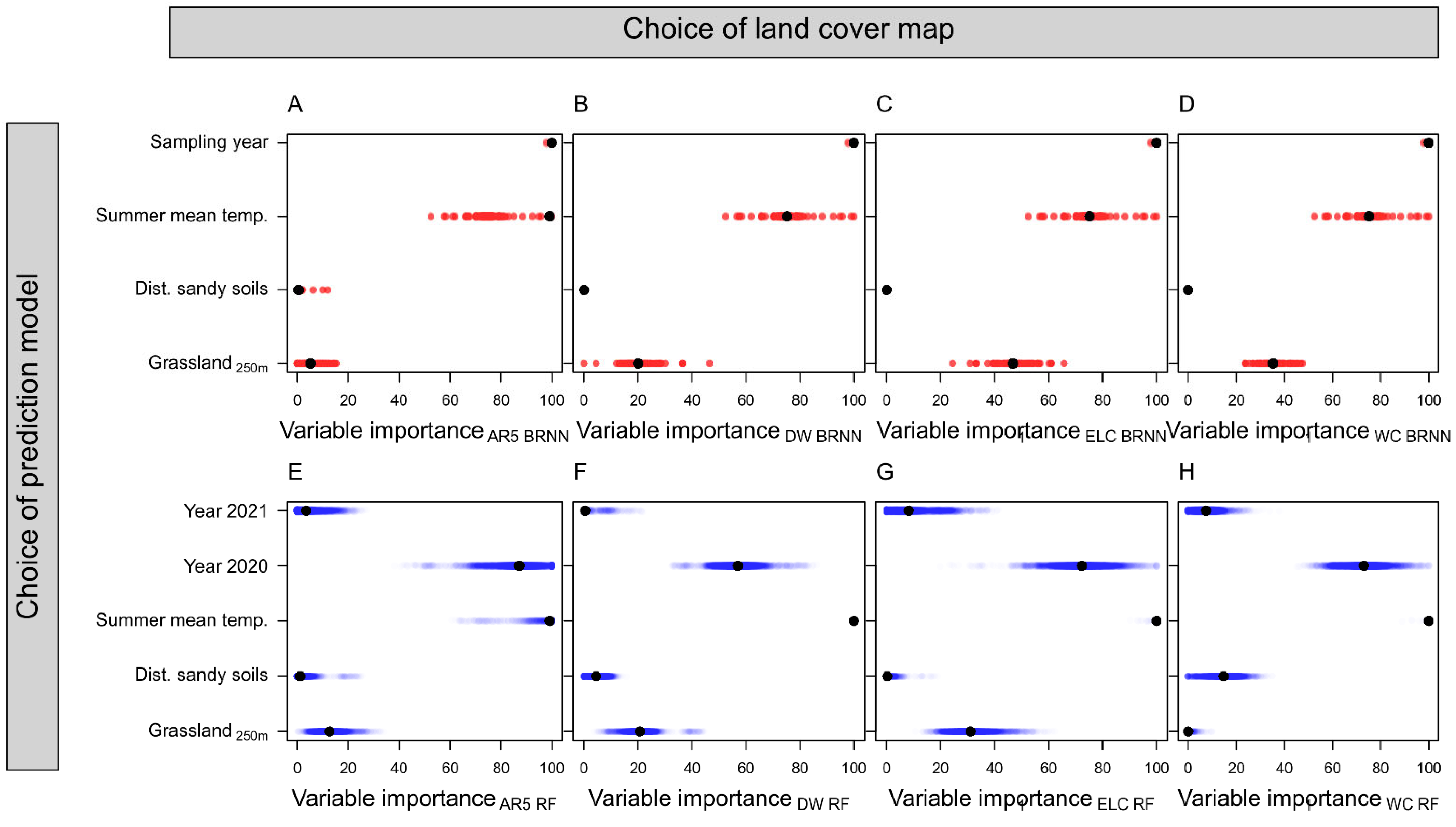
3. Results
4. Discussion
5. Conclusions
Author Contributions
Funding
Data Availability Statement
Acknowledgments
Conflicts of Interest
References
- Johnson, C.N.; Balmford, A.; Brook, B.W.; Buettel, J.C.; Galetti, M.; Guangchun, L.; Wilmshurst, J.M. Biodiversity Losses and Conservation Responses in the Anthropocene. Science 2017, 356, 270–275. [Google Scholar] [CrossRef] [PubMed]
- Edens, B.; Maes, J.; Hein, L.; Obst, C.; Siikamaki, J.; Schenau, S.; Javorsek, M.; Chow, J.; Chan, J.Y.; Steurer, A.; et al. Establishing the SEEA Ecosystem Accounting as a Global Standard. Ecosyst. Serv. 2022, 54, 101413. [Google Scholar] [CrossRef]
- Schmeller, D.S.; Böhm, M.; Arvanitidis, C.; Barber-Meyer, S.; Brummitt, N.; Chandler, M.; Chatzinikolaou, E.; Costello, M.J.; Ding, H.; García-Moreno, J.; et al. Building Capacity in Biodiversity Monitoring at the Global Scale. Biodivers. Conserv. 2017, 26, 2765–2790. [Google Scholar] [CrossRef] [Green Version]
- Villero, D.; Pla, M.; Camps, D.; Ruiz-Olmo, J.; Brotons, L. Integrating Species Distribution Modelling into Decision-Making to Inform Conservation Actions. Biodivers. Conserv. 2017, 26, 251–271. [Google Scholar] [CrossRef]
- Guisan, A.; Tingley, R.; Baumgartner, J.B.; Naujokaitis-Lewis, I.; Sutcliffe, P.R.; Tulloch, A.I.T.; Regan, T.J.; Brotons, L.; McDonald-Madden, E.; Mantyka-Pringle, C.; et al. Predicting Species Distributions for Conservation Decisions. Ecol. Lett. 2013, 16, 1424–1435. [Google Scholar] [CrossRef]
- McShea, W.J. What Are the Roles of Species Distribution Models in Conservation Planning? Environ. Conserv. 2014, 41, 93–96. [Google Scholar] [CrossRef] [Green Version]
- Harvey, J.A.; Heinen, R.; Armbrecht, I.; Basset, Y.; Baxter-Gilbert, J.H.; Bezemer, T.M.; Böhm, M.; Bommarco, R.; Borges, P.A.; Cardoso, P. International Scientists Formulate a Roadmap for Insect Conservation and Recovery. Nat. Ecol. Evol. 2020, 4, 174–176. [Google Scholar] [CrossRef]
- Senapathi, D.; Goddard, M.A.; Kunin, W.E.; Baldock, K.C. Landscape Impacts on Pollinator Communities in Temperate Systems: Evidence and Knowledge Gaps. Funct. Ecol. 2017, 31, 26–37. [Google Scholar] [CrossRef] [Green Version]
- Norwegian Ministries. National Pollinator Strategy A Strategy for Viable Populations of Wild Bees and Other Pollinating Insects; Norwegian Government Security and Service Organisation: Oslo, Norway, 2018; p. 67.
- IPBES. The Assessment Report of the Intergovernmental Science-Policy Platform on Biodiversity and Ecosystem Services on Pollinators, Pollination and Food Production; Potts, S.G., Imperatriz-Fonseca, V.L., Ngo, H.T., Eds.; Secretariat of the Intergovernmental Science-Policy Platform on Biodiversity and Ecosystem Services: Bonn, Germany, 2016; p. 552. [Google Scholar] [CrossRef]
- Sydenham, M.A.K.; Venter, Z.S.; Eldegard, K.; Moe, S.R.; Steinert, M.; Staverløkk, A.; Dahle, S.; Skoog, D.I.J.; Hanevik, K.A.; Skrindo, A.; et al. High Resolution Prediction Maps of Solitary Bee Diversity Can Guide Conservation Measures. Landsc. Urban Plan. 2022, 217, 104267. [Google Scholar] [CrossRef]
- Zurell, D.; Thuiller, W.; Pagel, J.; Cabral, J.S.; Münkemüller, T.; Gravel, D.; Dullinger, S.; Normand, S.; Schiffers, K.H.; Moore, K.A.; et al. Benchmarking Novel Approaches for Modelling Species Range Dynamics. Glob. Change Biol. 2016, 22, 2651–2664. [Google Scholar] [CrossRef] [Green Version]
- Randin, C.F.; Ashcroft, M.B.; Bolliger, J.; Cavender-Bares, J.; Coops, N.C.; Dullinger, S.; Dirnböck, T.; Eckert, S.; Ellis, E.; Fernández, N.; et al. Monitoring Biodiversity in the Anthropocene Using Remote Sensing in Species Distribution Models. Remote Sens. Environ. 2020, 239, 111626. [Google Scholar] [CrossRef]
- Venter, Z.S.; Sydenham, M.A.K. Continental-Scale Land Cover Mapping at 10 m Resolution Over Europe (ELC10). Remote Sens. 2021, 13, 2301. [Google Scholar] [CrossRef]
- Brown, C.F.; Brumby, S.P.; Guzder-Williams, B.; Birch, T.; Hyde, S.B.; Mazzariello, J.; Czerwinski, W.; Pasquarella, V.J.; Haertel, R.; Ilyushchenko, S.; et al. Dynamic World, Near Real-Time Global 10 m Land Use Land Cover Mapping. Sci. Data 2022, 9, 251. [Google Scholar] [CrossRef]
- Zanaga, D.; Van De Kerchove, R.; De Keersmaecker, W.; Souverijns, N.; Brockmann, C.; Quast, R.; Wevers, J.; Grosu, A.; Paccini, A.; Vergnaud, S.; et al. ESA WorldCover 10 m 2020 V100. Zenodo 2021. [Google Scholar] [CrossRef]
- Tulbure, M.G.; Hostert, P.; Kuemmerle, T.; Broich, M. Regional Matters: On the Usefulness of Regional Land-Cover Datasets in Times of Global Change. Remote Sens. Ecol. Conserv. 2022, 8, 272–283. [Google Scholar] [CrossRef]
- Bjørdal, I.; Bjørkelo, K. AR5 Klassifikasjonssystem: Klassifikasjon Av Arealressurser. In Håndbok Fra Skog Og Landskap; The Norwegian Institute of Bioeconomy Research: Ås, Norway, 2006. [Google Scholar]
- Noriega, J.A.; Hortal, J.; Azcárate, F.M.; Berg, M.P.; Bonada, N.; Briones, M.J.I.; Del Toro, I.; Goulson, D.; Ibanez, S.; Landis, D.A.; et al. Research Trends in Ecosystem Services Provided by Insects. Basic Appl. Ecol. 2018, 26, 8–23. [Google Scholar] [CrossRef] [Green Version]
- Prather, C.M.; Pelini, S.L.; Laws, A.; Rivest, E.; Woltz, M.; Bloch, C.P.; Del Toro, I.; Ho, C.; Kominoski, J.; Newbold, T.S. Invertebrates, Ecosystem Services and Climate Change. Biol. Rev. 2013, 88, 327–348. [Google Scholar] [CrossRef]
- Gallai, N.; Salles, J.-M.; Settele, J.; Vaissière, B.E. Economic Valuation of the Vulnerability of World Agriculture Confronted with Pollinator Decline. Ecol. Econ. 2009, 68, 810–821. [Google Scholar] [CrossRef]
- Losey, J.E.; Vaughan, M. The Economic Value of Ecological Services Provided by Insects. Bioscience 2006, 56, 311–323. [Google Scholar] [CrossRef] [Green Version]
- Smith, T.J.; Saunders, M.E. Honey Bees: The Queens of Mass Media, despite Minority Rule among Insect Pollinators. Insect Conserv. Divers. 2016, 9, 384–390. [Google Scholar] [CrossRef]
- Hallmann, C.A.; Sorg, M.; Jongejans, E.; Siepel, H.; Hofland, N.; Schwan, H.; Stenmans, W.; Müller, A.; Sumser, H.; Hörren, T. More than 75 Percent Decline over 27 Years in Total Flying Insect Biomass in Protected Areas. PLoS ONE 2017, 12, e0185809. [Google Scholar] [CrossRef] [PubMed] [Green Version]
- Seibold, S.; Gossner, M.M.; Simons, N.K.; Blüthgen, N.; Müller, J.; Ambarlı, D.; Ammer, C.; Bauhus, J.; Fischer, M.; Habel, J.C. Arthropod Decline in Grasslands and Forests Is Associated with Landscape-Level Drivers. Nature 2019, 574, 671–674. [Google Scholar] [CrossRef] [PubMed]
- Wagner, D.L.; Grames, E.M.; Forister, M.L.; Berenbaum, M.R.; Stopak, D. Insect Decline in the Anthropocene: Death by a Thousand Cuts. Proc. Natl. Acad. Sci. USA 2021, 118, e2023989118. [Google Scholar] [CrossRef] [PubMed]
- Zattara, E.E.; Aizen, M.A. Worldwide Occurrence Records Suggest a Global Decline in Bee Species Richness. One Earth 2021, 4, 114–123. [Google Scholar] [CrossRef]
- Orr, M.C.; Hughes, A.C.; Chesters, D.; Pickering, J.; Zhu, C.-D.; Ascher, J.S. Global Patterns and Drivers of Bee Distribution. Curr. Biol. 2021, 31, 451–458. [Google Scholar] [CrossRef]
- Sydenham, M.A.K.; Eldegard, K.; Venter, Z.S.; Evju, M.; Åström, J.; Rusch, G.M. Priority Maps for Pollinator Habitat Enhancement Schemes in Semi-Natural Grasslands. Landsc. Urban Plan. 2022, 220, 104354. [Google Scholar] [CrossRef]
- Westrich, P. Habitat Requirements of Central European Bees and the Problems of Partial Habitats; Academic Press Limited: Cambridge, MA, USA, 1996; Volume 18, pp. 1–16. [Google Scholar]
- Woodard, S.H.; Jha, S. Wild Bee Nutritional Ecology: Predicting Pollinator Population Dynamics, Movement, and Services from Floral Resources. Curr. Opin. Insect Sci. 2017, 21, 83–90. [Google Scholar] [CrossRef]
- Carrié, R.; Lopes, M.; Ouin, A.; Andrieu, E. Bee Diversity in Crop Fields Is Influenced by Remotely-Sensed Nesting Resources in Surrounding Permanent Grasslands. Ecol. Indic. 2018, 90, 606–614. [Google Scholar] [CrossRef]
- Requier, F.; Leonhardt, S.D. Beyond Flowers: Including Non-Floral Resources in Bee Conservation Schemes. J. Insect Conserv. 2020, 24, 5–16. [Google Scholar] [CrossRef]
- Antoine, C.M.; Forrest, J.R. Nesting Habitat of Ground-nesting Bees: A Review. Ecol. Entomol. 2021, 46, 143–159. [Google Scholar] [CrossRef]
- O’Connor, R.S.; Kunin, W.E.; Garratt, M.P.; Potts, S.G.; Roy, H.E.; Andrews, C.; Jones, C.M.; Peyton, J.M.; Savage, J.; Harvey, M.C. Monitoring Insect Pollinators and Flower Visitation: The Effectiveness and Feasibility of Different Survey Methods. Methods Ecol. Evol. 2019, 10, 2129–2140. [Google Scholar] [CrossRef]
- Hutchinson, L.A.; Oliver, T.H.; Breeze, T.D.; O’Connor, R.S.; Potts, S.G.; Roberts, S.P.; Garratt, M.P. Inventorying and Monitoring Crop Pollinating Bees: Evaluating the Effectiveness of Common Sampling Methods. Insect Conserv. Divers. 2022, 15, 299–311. [Google Scholar] [CrossRef]
- Droege, S.; Tepedino, V.J.; LeBuhn, G.; Link, W.; Minckley, R.L.; Chen, Q.; Conrad, C. Spatial Patterns of Bee Captures in North American Bowl Trapping Surveys. Insect Conserv. Divers. 2010, 3, 15–23. [Google Scholar] [CrossRef]
- Gorelick, N.; Hancher, M.; Dixon, M.; Ilyushchenko, S.; Thau, D.; Moore, R. Google Earth Engine: Planetary-Scale Geospatial Analysis for Everyone. Remote Sens. Environ. 2017, 202, 18–27. [Google Scholar] [CrossRef]
- Steffan-Dewenter, I.; Münzenberg, U.; Bürger, C.; Thies, C.; Tscharntke, T. Scale-dependent Effects of Landscape Context on Three Pollinator Guilds. Ecology 2002, 83, 1421–1432. [Google Scholar] [CrossRef]
- R Core Team. R: A Language and Environment for Statistical Computing 2021; R Core Team: Vienna, Austria, 2021. [Google Scholar]
- Lussana, C.; Tveito, O.; Uboldi, F. Three-dimensional Spatial Interpolation of 2 m Temperature over Norway. Q. J. R. Meteorol. Soc. 2018, 144, 344–364. [Google Scholar] [CrossRef]
- Geological Survey of Norway Løsmasser WMS. Available online: https://kartkatalog.geonorge.no/metadata/norges-geologiske-undersokelse/losmasser-wms/aa780848-5de8-4562-8f35-3d5c80ea8b48/ (accessed on 24 October 2022).
- Wright, M.N.; Wager, S.; Probst, P. R Package, Version 0.12; Ranger: A Fast Implementation of Random Forests; R Core Team: Vienna, Austria, 2020; Volume 1.
- Rodriguez, P.P.; Gianola, D. R Package, Version 0.6; BRNN: Bayesian Regularization for Feed-Forward Neural Networks; R Core Team: Vienna, Austria, 2016.
- Kuhn, M. Building Predictive Models in R Using the Caret Package. J. Stat. Softw. 2008, 28, 1–26. [Google Scholar] [CrossRef] [Green Version]
- Singh, V.; Pencina, M.; Einstein, A.J.; Liang, J.X.; Berman, D.S.; Slomka, P. Impact of Train/Test Sample Regimen on Performance Estimate Stability of Machine Learning in Cardiovascular Imaging. Sci. Rep. 2021, 11, 14490. [Google Scholar] [CrossRef]
- Greenwell, B.M. Pdp: An R Package for Constructing Partial Dependence Plots. R J. 2017, 9, 421. [Google Scholar] [CrossRef] [Green Version]
- Nkhwanana, N.; Adam, E.; Ramoelo, A. Assessing the Utility of Sentinel-2 MSI in Mapping an Encroaching Serephium Plumosum in South African Rangeland. Appl. Geomat. 2022, 14, 435–449. [Google Scholar] [CrossRef]
- De Simone, W.; Allegrezza, M.; Frattaroli, A.R.; Montecchiari, S.; Tesei, G.; Zuccarello, V.; Di Musciano, M. From Remote Sensing to Species Distribution Modelling: An Integrated Workflow to Monitor Spreading Species in Key Grassland Habitats. Remote Sens. 2021, 13, 1904. [Google Scholar] [CrossRef]
- Olofsson, P.; Foody, G.M.; Herold, M.; Stehman, S.V.; Woodcock, C.E.; Wulder, M.A. Good Practices for Estimating Area and Assessing Accuracy of Land Change. Remote Sens. Environ. 2014, 148, 42–57. [Google Scholar] [CrossRef]
- Marshall, L.; Beckers, V.; Vray, S.; Rasmont, P.; Vereecken, N.J.; Dendoncker, N. High Thematic Resolution Land Use Change Models Refine Biodiversity Scenarios: A Case Study with Belgian Bumblebees. J. Biogeogr. 2021, 48, 345–358. [Google Scholar] [CrossRef]
- Griffiths, P.; Nendel, C.; Pickert, J.; Hostert, P. Towards National-Scale Characterization of Grassland Use Intensity from Integrated Sentinel-2 and Landsat Time Series. Remote Sens. Environ. 2020, 238, 111124. [Google Scholar] [CrossRef]
- Coops, N.C.; Waring, R.H.; Plowright, A.; Lee, J.; Dilts, T.E. Using Remotely-Sensed Land Cover and Distribution Modeling to Estimate Tree Species Migration in the Pacific Northwest Region of North America. Remote Sens. 2016, 8, 65. [Google Scholar] [CrossRef] [Green Version]
- Venter, Z.S.; Barton, D.N.; Chakraborty, T.; Simensen, T.; Singh, G. Global 10 mL and Use Land Cover Datasets: A Comparison of Dynamic World, World Cover and Esri Land Cover. Remote Sens. 2022, 14, 4101. [Google Scholar] [CrossRef]
- White, E.R. Minimum Time Required to Detect Population Trends: The Need for Long-Term Monitoring Programs. BioScience 2019, 69, 40–46. [Google Scholar] [CrossRef] [Green Version]


Disclaimer/Publisher’s Note: The statements, opinions and data contained in all publications are solely those of the individual author(s) and contributor(s) and not of MDPI and/or the editor(s). MDPI and/or the editor(s) disclaim responsibility for any injury to people or property resulting from any ideas, methods, instructions or products referred to in the content. |
© 2023 by the authors. Licensee MDPI, Basel, Switzerland. This article is an open access article distributed under the terms and conditions of the Creative Commons Attribution (CC BY) license (https://creativecommons.org/licenses/by/4.0/).
Share and Cite
Venter, Z.S.; Roos, R.E.; Nowell, M.S.; Rusch, G.M.; Kvifte, G.M.; Sydenham, M.A.K. Comparing Global Sentinel-2 Land Cover Maps for Regional Species Distribution Modeling. Remote Sens. 2023, 15, 1749. https://doi.org/10.3390/rs15071749
Venter ZS, Roos RE, Nowell MS, Rusch GM, Kvifte GM, Sydenham MAK. Comparing Global Sentinel-2 Land Cover Maps for Regional Species Distribution Modeling. Remote Sensing. 2023; 15(7):1749. https://doi.org/10.3390/rs15071749
Chicago/Turabian StyleVenter, Zander S., Ruben E. Roos, Megan S. Nowell, Graciela M. Rusch, Gunnar M. Kvifte, and Markus A. K. Sydenham. 2023. "Comparing Global Sentinel-2 Land Cover Maps for Regional Species Distribution Modeling" Remote Sensing 15, no. 7: 1749. https://doi.org/10.3390/rs15071749