Present-Day Surface Deformation in North-East Italy Using InSAR and GNSS Data

Abstract

Geodetic data can detect and estimate deformation signals and rates due to natural and anthropogenic phenomena. In the present study, we focus on northeastern Italy, an area characterized by ~1.5–3 mm/yr of convergence rates due to the collision of Adria-Eurasia plates and active subsidence along the coasts. To define the rates and trends of tectonic and subsidence signals, we use a Multi-Temporal InSAR (MT-InSAR) approach called the Stanford Method for Persistent Scatterers (StaMPS), which is based on the detection of coherent and temporally stable pixels in a stack of single-master differential interferograms. We use Sentinel-1 SAR images along ascending and descending orbits spanning the 2015–2019 temporal interval as inputs for Persistent Scatterers InSAR (PSI) processing. We apply spatial-temporal filters and post-processing steps to reduce unrealistic results. Finally, we calibrate InSAR measurements using GNSS velocities derived from permanent stations available in the study area. Our results consist of mean ground velocity maps showing the displacement rates along the radar Line-Of-Sight for each satellite track, from which we estimate the east–west and vertical velocity components. Our results provide a detailed and original view of active vertical and horizontal displacement rates over the whole region, allowing the detection of spatial velocity gradients, which are particularly relevant to a better understanding of the seismogenic potential of the area. As regards the subsidence along the coasts, our measurements confirm the correlation between subsidence and the geological setting of the study area, with rates of ~2–4 mm/yr between the Venezia and Marano lagoons, and lower than 1 mm/yr near Grado.

1. Introduction

Space geodetic measurements are crucial in assessing natural and anthropogenic surface deformation, as they can detect and monitor spatially consistent deformation patterns at different length scales. Recent advances in space geodetic techniques allow measurement of ground displacement rates over large areas with millimeter accuracies. For example, geodetic data have been exploited to extract information on tectonic activity (e.g., interseismic displacement; Iran–Pakistan–India: [1,2,3,4]; California: [5,6,7]; Anatolia: [8,9,10,11]; Italy: [12,13,14,15,16]), investigations regarding subsidence (e.g., [17,18,19,20,21,22,23,24,25,26]), landslides and slope instabilities (e.g., [27,28,29,30]), sinkholes (e.g., [31]), volcanic processes (e.g., [32,33,34]), monitoring of infrastructures, reservoirs, and mining activities (e.g., [35,36,37,38]).

Global Navigation Satellite Systems (GNSS) and Synthetic Aperture Radar Interferometry (InSAR) are today the most widely used methods for estimating and monitoring ground displacements (e.g., [39,40]). GNSS provides highly accurate, punctual, daily 3D surface displacement and velocity information referring to a receiver on the ground [41]. Conversely, spaceborne MT-InSAR (Multi-temporal InSAR) generates a 1D ground deformation time-series in the radar line-of-sight (LOS), with a temporal sampling of several days, but with a high spatial density over areas containing several stable radar scatterers (e.g., man-made structures). In the last few years, the development and extensive use of new satellites and new algorithms have made it possible to detect tectonic, gravitative, hydrogeological, and anthropogenic deformation signals, even in areas exhibiting low displacement rates (e.g., [33,34,42,43]).

In northeastern Italy, the tectonic setting is characterized by two fold-and-thrust systems, i.e., the Southeastern Alps and the External Dinarides, and their foreland, i.e., the Venetian-Friulian plain (e.g., [44]; Figure 1). The recent tectonic activity is characterized by active south verging thrusting and strike-slip faulting in the Alpine (e.g., the 1976 Mw 6.4 Friuli earthquake) and Dinaric systems, respectively, as the result of the about N-S active convergence between the Adriatic and Eurasian plates, at 1.5–3 mm/yr [15,45,46,47,48,49,50,51].

Regarding the Venetian-Friulian plain and coastal areas, active subsidence has been described in response to natural (sediment compaction) and anthropogenic causes (e.g., urbanization or groundwater and gas pumping) [18,52].

Based on GNSS and MT-InSAR data, previous studies in northeastern Italy estimated ground displacement rates and correlated them to the ongoing processes. The geodetically estimated convergence rates have been used to define the geometrical and kinematic behaviors of the active faults and their seismogenic potential (e.g., [12,15,16,53,54,55,56]).

Several other studies used geodetic observations, focusing on non-tectonic processes affecting the study area. Rossi et al. [57,58,59] described transient deformation signals associated with pore pressure variations in rocks in response to tectonic stress. Stocchi et al. [60] estimated the post-glacial isostatic rebound along the Alpine belt as ~1/3 of the measured vertical rates. Devoti et al. and Serpelloni et al. [61,62] revealed horizontal non-tectonic and non-seasonal ground deformation signals due to hydrologic flux in karstic areas in response to rainfall and groundwater flow, also describing a correlation between hydrological deformation transients and background seismicity [63]. Regarding the deformation rates along the plain and coasts, other studies have estimated active vertical subsidence, also posing a problem with coastal hazards and flooding [18,19,21,24,64,65,66].

Figure 1. Seismotectonic map of the study area. (A) The map shows the seismicity and tectonics of the region. The blue-purple circles represent the instrumental seismicity for the 2000–2017 time span, provided by OGS bulletins (URL: http://www.crs.inogs.it/bollettino/RSFVG (accessed on 31 August 2020)) with focal mechanisms of the most important historical events [15,48,49]. (B) The map shows the tectonics and paleogeography of the area. (AR: Arba-Ragogna thrust; BL: Belluno thrust; BV: Bassano-Valdobbiadene thrust; CA: Cansiglio thrust; FS: Fella-Sava line; ID: Idrija fault; MD: Medea thrust; MT: Montello thrust; PAF: Periadriatic fault; PM: Polcenigo-Maniago thrust; PR: Predjama fault; PT: Pozzuolo thrust; RA: Raša fault; RV: Ravne Fault; ST: Susans-Tricesimo thrust; TBC: Thiene-Bassano-Cornuda thrusts; VS: Valsugana thrust). (C) Simplified geological map with stratigraphic column (Modified from: [67]).

Figure 1. Seismotectonic map of the study area. (A) The map shows the seismicity and tectonics of the region. The blue-purple circles represent the instrumental seismicity for the 2000–2017 time span, provided by OGS bulletins (URL: http://www.crs.inogs.it/bollettino/RSFVG (accessed on 31 August 2020)) with focal mechanisms of the most important historical events [15,48,49]. (B) The map shows the tectonics and paleogeography of the area. (AR: Arba-Ragogna thrust; BL: Belluno thrust; BV: Bassano-Valdobbiadene thrust; CA: Cansiglio thrust; FS: Fella-Sava line; ID: Idrija fault; MD: Medea thrust; MT: Montello thrust; PAF: Periadriatic fault; PM: Polcenigo-Maniago thrust; PR: Predjama fault; PT: Pozzuolo thrust; RA: Raša fault; RV: Ravne Fault; ST: Susans-Tricesimo thrust; TBC: Thiene-Bassano-Cornuda thrusts; VS: Valsugana thrust). (C) Simplified geological map with stratigraphic column (Modified from: [67]).

As the geodetic sensors and processing techniques have quickly improved the accuracy and precision of ground deformation measurements over the years, our goal in this study is to update the geodetic velocity field in northeastern Italy and its surrounding regions by integrating GNSS and MT-InSAR data. The resulting mean ground velocity maps allow for the detection of spatial gradients of the velocities across the area during the observation period, offering new clues about active tectonics and subsidence.

Geological Setting

To understand the nature of ground deformation recorded by space geodetic measurements in the study area, it is central to consider the geological features in terms of rock type, recent tectonic activity (e.g., seismicity), and the natural and anthropogenic phenomena acting near or close to the coasts.

The stratigraphic sequence consists of a Paleozoic crystalline and metamorphic basement covered by thick Mesozoic carbonate and terrigenous rock sequences (e.g., [68,69,70]). Tertiary rocks derive from terrigenous sediments (e.g., turbiditic and generic clastic deposits) related to the erosion of growing Alpine and Dinaric chains. Quaternary shallow-marine and alluvial plain deposits complete the sequence [68,69,71,72] (Figure 1C).

The present-day tectonic setting of the region derives from the superposition of different tectonic phases (Figure 1A). During the Mesozoic, an extensional phase generated a horst and graben system. The development of thick carbonate platforms took place from Triassic to Cretaceous. During the Early Jurassic, a nearly NS-oriented basin, namely the Belluno-Northern Adriatic basin, separated the two carbonate platforms, i.e., the Trento Platform to the west and the Friuli Platform to the east [68,70,73] (Figure 1B). Finally, during the Paleogene, a small and shallow basin was formed in the northern part of the Friuli platform [74].

From the Cenozoic, three main compressional phases occurred in the area, causing the formation and development of the Alpine and Dinaric chains.

The first compressional event coincided with the inception of the Alpine orogeny. In particular, in the study region, the first contractional structures developed from the Cretaceous to Late Eocene, resulting in NW–SE-trending Dinarides fold and thrust systems (e.g., [75,76]). From the Serravallian to Messinian, a slightly differently oriented contractional phase generated ~EW-oriented fold and thrust systems of the Southern Alps [75,77]. Finally, from Late Messinian to the present day, new southeast-verging thrust-and-fold systems developed in the central-eastern sector of the Southern Alps due to the rotation of the maximum stress axis northwards [75,76]. Meanwhile, major strike-slip faults developed in the eastern sector, with some partially reusing segments of pre-existing thrusts [78].

ENE-trending, southeast-verging, folds, and thrusts dominate the present-day tectonic setting of the western area (Long. 11.6°–12.8°), such as the Valsugana thrust, the Belluno thrust, the Bassano-Valdobbiadene thrust in the inner sectors, and the external thrust front, including, from west to east, the Thiene-Bassano-Cornuda, Montello, Cansiglio, Polcenigo-Maniago, and Arba-Ragogna Thrusts [79,80] (Figure 1B). In the sector where the interaction of the Alpine and Dinaric systems is most active (Long. 12.8°–13.5°), the south-verging thrust-and-fold system tends to be mainly E-W-oriented, as, for example, the Periadriatic thrust and the Susans-Tricesimo line [79,80,81]. Several NW-SE-oriented, sub-vertical, dextral strike-slip faults belonging to the Dinaric system, such as Raša, Predjama, Idrija, and Ravne faults, are found in the eastern sector (Long. 13.5°–13.9°) [55,56,80,82] (Figure 1B). The Dinaric system is today interrupted along the Fella-Sava fault, a transpressional structure located in the northeastern sector that accommodates a large part of the right-lateral motion between the Eastern Southern Alps and the Eastern Alps [15]. In the Friulian Plain, buried by thick Quaternary sediments, there are south-verging thrusts, especially around Udine, such as the Udine-Buttrio and Medea thrusts (e.g., [80]).

The distribution of instrumental seismicity, as shown in Figure 1A for the 2000–2017 time span along the study area, demonstrates that some of the previous structures are still active. Historical seismicity and geological evidence confirm the activity of these structures, even suggesting the generation of moderate/strong earthquakes [79,80,83]. Among all the events, we mention the 1976–1977 Friuli sequence (mainshock Mw 6.4) and the 1998 and 2004 Bovec-Krn earthquakes (Mw 5.6 and Mw 5.2) [45,46,47,79,84,85,86,87].

Regarding the Venetian-Friulian plain, the Pre-Quaternary thick sedimentary sequence (up to 1500 m) is derived from the erosion of the Dinaric and Alpine belts and is mainly composed of clay-silty layers with thin sandy layers (e.g., [18,72,88]).

The Quaternary deposits consist of consolidated sandy and silty-clay layers mainly related to alluvial and marine-lagoon environments, with a variable thickness from hundreds of meters to 3000 m moving from the northeast (i.e., the Friuli area) to the southwest (i.e., the Venezia lagoon) (e.g., [18,68,89]. In the Venezia lagoon area, sandy sediments are mainly distributed in the central sector. In contrast, more compressible clay sediments predominate in the northern and southern areas [88].

The unconsolidated Holocene deposits, characterized by a maximum thickness of a few tens of meters, present heterogeneous lithologies (sand, silt, and clay) in response to marine ingression and fluvial actions [18,89].

2. Materials and Methods

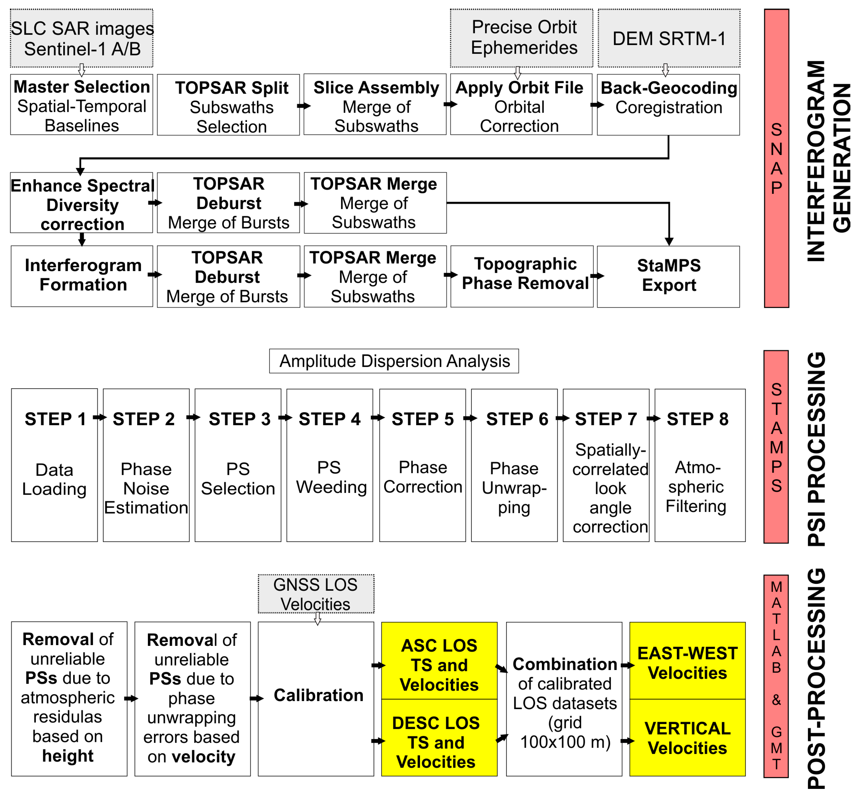
2.1. InSAR Processing

To obtain ground velocities in the study area, we use C-band SAR images acquired by the Sentinel-1 A/B satellites in Interferometric Wide swath mode (IW). This imaging mode is characterized by a swath width of 250 km and a spatial resolution of 5 × 20 m in the range and azimuth directions [90,91]. We collect Single-Look Complex (SLC) images along ascending track 44 and descending track 95, spanning late March 2015 to December 2019 (Figure 2). We use the Stanford Method for Persistent Scatterers (StaMPS), which enables the identification of stable radar targets in urban and non-urban environments characterized by variable displacement rates [32,92].

The generation of mean velocity maps using InSAR data requires three main steps: (1) preprocessing based on the open-source snap2stamps package [93], (2) PSI processing with StaMPS software, and (3) post-processing operations (Figure 3).

The first step enables the generation of a stack of coregistered images and differential interferograms referred to a single reference image. Reference images are on 7 August 2017 and 11 August 2017 for the ascending and descending datasets, respectively. We use precise orbit ephemerides, automatically downloaded by SNAP, for orbital refinement and the 1-arcsec Shuttle Radar Topography Mission (SRTM) Digital Elevation Model (DEM) for image coregistration and topographic phase removal.

StaMPS processing consists of several steps (Figure 3). A preliminary selection of Persistent Scatterer (PS) candidates is carried out by applying an amplitude dispersion threshold of 0.4 [32,91,92]. The area of interest is then divided into 3 × 3 patches, with an overlap of 50 pixels, which are processed in parallel in subsequent steps to improve computational efficiency. For each data patch, we load the input data (processing step #1), estimate the phase noise for each pixel in every interferogram (step #2), select the potential PS candidates based on their phase noise characteristics (step #3), and remove potential outliers (step #4). After the phase correction for spatially uncorrelated DEM errors, the patches are merged and resampled with a sampling of 100 m (step #5). During step #6, we compute 3D phase unwrapping based on the algorithm described by [32] using the statistical-cost, network-flow phase-unwrapping algorithm (SNAPHU) by [94], implemented in StaMPS software. By setting the unwrapping resampling grid (unwrap_grid_size) at 100 m, we test two different values for the window size of the Goldstein filter (unwrap_gold_n_win) (32 × 32 and 64 × 64 pixels) [95] to compare and evaluate the results, namely 100_32 and 100_64 datasets. After the unwrapping, the spatially correlated DEM errors and the atmospheric and orbital error contributions of the Reference image are estimated (step #7). Finally, during step #8, we apply a high pass filter in time (scn_time_win = 45 days) and a low pass filter in space (scn_wavelength = 400 m) to remove potential atmospheric contributions related to Secondary images [37,96,97,98]. Finally, after defining a common reference point on a tectonically and vertically stable area (Long. 12.84°E; Lat. 45.95°N) for both the ascending and descending radar tracks, we obtain two displacement time series in the radar LOS direction with respect to the reference point.

The third processing block in Figure 3 consists of a set of post-processing operations to remove unreliable measurements in the study area.

First, we remove PSs potentially affected by residual atmospheric contributions correlated with height. Although the use of spatial-temporal filters can mitigate turbulent atmospheric delays, which are considered spatially correlated and temporally uncorrelated [32,97,98], this method might not be so effective in the case of temporally correlated stratified tropospheric contributions [99]. Hence, considering the study area, we remove the PSs whose difference in height with respect to the reference point was higher than 1000 m to reduce the atmospheric propagation effects correlated with topographic height [99].

Second, we compare the results obtained for each radar track using the two different Goldstein filtering window size parameters and remove the PSs with a velocity (displacement rate) difference higher than a given threshold. Considering the convergence rates of ~1.5–3 mm/yr in the study area, we define the threshold at 1 mm/yr. Finally, we remove pixels with a multi-temporal coherence value < 0.6. For the ascending track, we mask out an area close to the Carnic Alps, characterized by spatially correlated PSs, showing a significant velocity difference (mean value of 5 mm/yr) with respect to the adjacent PSs.

Figure 4A,B shows the resulting mean LOS velocity maps for both tracks.

2.2. GNSS-InSAR Calibration

InSAR measurements are relative both in time (w.r.t. the first image of the data stack) and in space (w.r.t. to the selected spatial reference), and large-scale deformation gradients measured with this technique are unreliable, mostly due to atmospheric propagation effects and orbital uncertainties, which cannot be entirely corrected with the processing steps described in the previous section [100]. Therefore, the InSAR measurements should be calibrated and validated with independent ground-based observations in order to assess the reliability of the data. Because of the high accuracy of the measurements [41], GNSS data are usually employed to calibrate InSAR datasets. In the present work, we used GNSS velocities among different approaches to calibrate InSAR measurements [16,24,101,102,103].

The GNSS velocities used have been obtained by processing data from continuous stations belonging to several public and private networks, following the approach described in [104] and are part of a Euro-Mediterranean geodetic solution (e.g., [105]).

As reported in [104], GNSS processing consists of three steps:

(1)

GPS phase reduction and generation of loosely constrained sub-networks solutions using GAMIT [106];

(2)

Combination of daily subnet solutions and realization of positions in specific reference frames using GLOBK [106];

(3)

Analysis of time-series using QOCA (URL: http://qoca.jpl.nasa.gov (accessed on 20 March 2023)).

Starting from the displacement time series in the 2000–2020 time span, realized in the IGb14 reference frame (URL: https://lists.igs.org/pipermail/igsmail/2020/007917.html (accessed on 20 March 2023)), we estimate linear velocities, seasonal (annual and semi-annual) signals, and eventual instrumental offsets due to equipment changes for sites with a minimum observational period of 2.5 years to minimize possible biases in the linear trend estimation due to seasonal signals [107] and non-seasonal hydrological deformation signals [62].

The horizontal velocities in Figure 2 refer to an Adria-fixed reference frame considering the rotation pole from [15].

Given the two geodetic datasets, we first project the GNSS 3D velocity vectors along the SAR LOS directions for each track to calibrate the SAR measurements using the GNSS velocities. Since GNSS sites and PSs are not usually located in the same spot, we then calculate the mean and the standard deviation velocity of all PSs located within a given radius from each GNSS station to compare the two geodetic datasets.

The selection of GNSS stations is a crucial step that can meaningfully affect calibration. Hence, the GNSS stations used for calibration are chosen based on the following criteria:

• InSAR-GNSS temporal coverage overlapping;
• GNSS data continuity;
• InSAR-GNSS spatial colocation;
• Low spatial variability underlying the deformation field.

Concerning criterion #1, we consider the SAR observation interval, namely 2015–2019, as the reference period, thus excluding GNSS stations whose data acquisitions terminated before 2015. Similarly, for condition #2, we define a minimum period of 2.5 yr within the same temporal interval by excluding the GNSS stations having shorter time series. We fix these two criteria to improve the comparison between InSAR and GNSS data in the same reference period (2015–2019).

We run different tests by varying the radius value, namely 200, 400, 600, and 800 m, counting the number of detected PSs, and calculating the standard deviation of their ground velocity values. To guarantee a minimum number of PSs around each GNSS station, we assume the minimum PS number below which 10% of the values fall (criterion #3) as a threshold. Moreover, we fix the standard deviation threshold at 1 mm/yr to limit the spatial variability (criterion #4). Hence, considering all radii, we exclude the GNSS stations for which there are few PSs and high spatial variability in PSs velocities.

We retain 43 GNSS stations for the LOS datasets distributed in the study area (Figure 4A,B).

After the selection, we exploit the GNSS velocity values to perform the calibration, estimating a vertical offset due to the different reference frames between InSAR and GNSS, and allowing for image-wide trends due to orbital uncertainties and atmospheric propagation [108,109]. Both a planar [110] and a quadratic ramp calibration model [111,112] are tested by fitting the InSAR-GNSS velocity differences in a least-squares sense.

The processing settings described in the previous section, namely two processing runs using different Goldstein filter parameters (window sizes of 32 × 32 and 64 × 64 pixels, respectively), and the different GNSS-calibration settings, namely using different search radii (200, 400, 600, and 800 m) and two calibration error models (linear and quadratic), yield 16 different calibrated deformation products for each track, which have been evaluated based on the statistical comparison with the GNSS data (Tables S1 and S2).

In particular, we use the standard deviation and correlation coefficient values of the InSAR-GNSS residuals as quality parameters. Considering the lower standard deviation and the higher correlation coefficient of the residuals, we finally find the best calibrated LOS datasets to be those based on a quadratic calibration error model, a search radius of 600 m around each GNSS station, and a Goldstein filter window size of 64 (Tables S1 and S2). The standard deviation values of the resulting solutions are 0.68 and 0.56 mm/yr for the ascending and descending datasets, respectively. We use these values to define the accuracy of the calibrated InSAR measurements (e.g., [7]).

The correlation plots also state good agreement and a positive correlation between the geodetic measurements (Figure S1).

To better visualize the geodetic surface velocities in the study area, we obtain the horizontal (east–west) and vertical velocity maps by combing the two resulting LOS datasets. After the definition of a 100 × 100 m regular grid, we calculate the mean LOS velocities of all PSs within each grid cell in both datasets $(\Delta d_{asc}and\Delta d_{desc}$), we extract the values of the local incidence angle ($\theta$) (positive from the vertical) and the azimuth of the satellite heading vector $\left(\phi \right)$ (positive clockwise from the North) and we apply the following formula [113]:

$$\left(\begin{array}{c}\Delta d_{asc}\\ \Delta d_{desc} \end{array}\right)=\left(\begin{array}{c}-\cos {\phi }_{asc}\sin {\theta }_{asc} \sin {\phi }_{asc}\sin {\theta }_{asc} \cos {\theta }_{asc}\\ -\cos {\phi }_{desc}\sin {\theta }_{desc} \sin {\phi }_{desc}\sin {\theta }_{desc} \cos {\theta }_{desc}\end{array}\right)\left(\begin{array}{c}{\mathsf{\Delta }}_E\\ {\mathsf{\Delta }}_U\end{array}\right)$$

(1)

Finally, we compare the InSAR-GNSS velocities after the decomposition (Table S3; Figure S2). As done for the calibrated LOS products, we compute the mean velocity of the PSs within a radius of 600 m from each GNSS station, and we plot the InSAR-GNSS velocities (Figure S2). To evaluate the results, we use the standard deviation values and correlation coefficients of the InSAR-GNSS velocity residuals as quality parameters. Specifically, we obtain standard deviation and correlation coefficient values of 0.62 mm/yr and 0.55, respectively, for the east–west component and 0.61 mm/yr and 0.8, respectively, for the vertical dataset (Table S3).

3. Results

After the processing procedures explained in the previous section, the preliminary results consist of two calibrated LOS mean ground velocity maps, as shown in Figure 4C,D. During the linear estimation of the velocity for each PS, we also compute the standard deviation, which is characterized by mean values of 0.2 mm/yr for both LOS datasets, indicating low spatial variability of the InSAR displacement measurements w.r.t. a linear model (Table S4; Figure S3).

Due to the decorrelation (i.e., the presence of vegetated areas) and the removal of unreliable values during the post-processing operations, the final products show a lower PSs density across the mountain regions with respect to the plain, the intermontane valleys, and the coastal areas. However, the distribution of PSs enables the clear detection of gradients and deformation patterns in the study area.

Based on the E-W velocity map (Figure 5A), we report a general eastwards ground motion that increases northeastward by reaching ~1–2 mm/yr around Villach. Positive rates characterize the Venetian-Friulian plain, especially moving toward the mountain belt, although west of Venezia, we record displacement rates of 0.5–1 mm/yr in the opposite direction. We also observe westward displacement rates in the Dolomites area, with average values of 1–2 mm/yr, reaching locally up to 2 mm/yr.

The northern Friuli, the Austrian area, and the eastern Slovenian sector are characterized by eastward velocities at rates of ~1–2 mm/yr, decreasing southeastward (Figure 5A). Finally, the area east of Udine, across the Italian–Slovenian border, records a westward motion (0.5–1 mm/yr).

Regarding vertical velocities (Figure 5B), the Venetian-Friulian plain and the northern Adriatic coasts are mainly affected by subsidence, with negative rates of 0.5–3 mm/yr, decreasing toward the inland. Moreover, we note the presence of subsidence along the major rivers and close to the mountain belt, with negative rates of 0.5–1 mm/yr.

From Grado-Marano Lagoon to Croatia, the coasts present negative ground velocities with lower rates, decreasing eastwards and inland (<1 mm/yr). However, we also detect local strong negative signals faster than 4 mm/yr, especially near harbors and industrial areas.

Positive vertical velocities increase northward toward the south Alpine belt (Figure 5B). We estimate an uplift of ~1–2 mm/yr, reaching locally up to >3 mm/yr between the Dolomites and the Carnic Alps. Between the Carnic and the Julian Alps, we record positive vertical rates higher than 2 mm/yr, decreasing southwards (eastern border Italia–Slovenia) and eastwards (i.e., Austria and Slovenia), with values up to 0.5–1 mm/yr (Figure 5B).

Finally, we observe a subsidence of ~1 mm/yr affecting the Slovenian area (west of Ljubliana) and the Austrian region (east of Villach). In contrast, the areas near Trieste and the Croatia–Slovenia border present an uplift with rates of 0.5–1 mm/yr.

We trace some profiles across three different sectors of the Southern Alps and northern Dinarides to study possible correlations between the geodetic signals (InSAR and GNSS) and active tectonic structures (Figure 6, Figure 7, Figure 8, Figure 9 and Figure 10).

The westernmost section crosses the south Alpine thrusts, starting from the Venetian plain (Figure 6). In this case, we plot only the vertical component of the detected signals along this section, as vertical motion prevails here (Figure 5). The Venetian coasts and the plain areas around San Donà and Noventa di Piave (SDNA and NOVE GNSS stations in Figure 6) record negative vertical rates of 1–3 mm/yr, with a minimum located close to the ERAC GNSS station (Figure 5B and Figure 6). Moving northward, the vertical velocity increases, reaching values of ±1 mm/yr close to the MT01 GNSS site. Similarly, GNSS stations record negative rates and a progressive increase in the vertical velocities along the profile. The first 50–60 km of the profile are characterized by thick post-middle Miocene to Quaternary terrigenous deposits according to the geological section modified from [69]. These areas also lack seismicity, as shown in Figure 6.

A significant positive gradient of about 1 mm/yr between the VITT GNSS station and the Belluno Valley (BLNO–BL01 GNSS stations) is recorded by InSAR and GNSS measurements. Observing the seismicity and tectonic structures (Figure 6), we note the presence of clusters characterized by moderate-small earthquakes with a hypocentral depth of 10–15 km. The recent seismic activity concentrated on the main thrusts’ deeper portions, especially the Montello, Bassano-Valdobbiadene, and Belluno Thrusts.

Regarding the second profile across the Carnic-Julian Alps, we note negative vertical rates of 1–3 mm/yr along the coasts, rapidly becoming positive with increasing values toward the stable area between the Udine and JOAN GNSS station (Figure 7). Based on the information provided by the geological section modified from [114], the area presents compressible terrigenous deposits over the Friulian carbonate platform, also characterized by low seismicity, with hypocentral depths of 5–15 km.

Moving toward the mountain belt, both geodetic measurements record a positive vertical velocity gradient with different estimated values. Indeed, the uplift recorded within 35 km along the profile around Tarvisio (TARV GNSS site) reaches up to 2.3 mm/yr instead of the lower GNSS values (~1 mm/yr). Considering the seismicity, we observe small events located at depths of 5-15 km near the south-verging thrusts and sub-vertical parallel strike-slip faults (i.e., Idrija and Ravne faults). Lower vertical rates characterize the areas near Villach, to the north of the Periadriatic fault, with values up to 1 mm/yr (Figure 7).

In the E-W velocity profile (Figure 8), the southern Friulian plain presents a westward movement (<1 mm/yr), whereas, to the north of Udine, a velocity increase is recorded (eastwards motion), with rates of about 1 mm/yr near Tarvisio (TARV GNSS site). In this case, GNSS measurements indicate a stable area and a moderate positive trend (<1 mm/yr Eastwards), respectively.

The last section crosses the sub-parallel, NW-SE trending Dinaric transcurrent and transpressional structures in the easternmost sector of the study area. Similar to the previous profiles, Figure 9 and Figure 10 show the vertical and east–west velocity components, respectively.

Starting from the vertical velocity profile (Figure 9), we observe a gradual increase in velocity from the Grado-Marano Lagoon (mean rate > −1 mm/yr) toward the inland, reaching rates lower than 1 mm/yr near the NOVG GNSS station. The area also shows a general eastward motion (Figure 10), except for a weak westward signal confined between MDEA and NOVG GNSS sites due to the effect of the deformation pattern recorded near Udine (see also Figure 8). Concerning the seismotectonic context, we note a few small seismic events localized between the crystalline basement and the carbonate units (depth of 10–15 km) and the presence of some buried thrusts and strike-slip faults located on the Friulian plain (Figure 9 and Figure 10).

Between the Raša and Idrija faults, we record an uplift and an eastward motion of ~1 mm/yr, as observed in Figure 9 and Figure 10.

We also identify a significant seismic activity at depth of 0–15 km, mainly concentrated around the Ravne fault.

North of the IDRI station, the velocity increases (Eastwards movement), reaching values up to 1.5 mm/yr in correspondence with the RADO station, which gradually decreases (~1 mm/yr) (Figure 10). Similarly, we record a positive vertical gradient of about 1.5 mm/yr within approximately 35 km along the profile, decreasing toward the valley of Villach in Austria (~0 mm/yr) (Figure 9). Even the GNSS data delineate similar trends in vertical and east–west velocity despite the lower estimated rates. Finally, the seismic data show a small cluster near the Fella-Sava fault at depths of 5–10 km.

4. Discussion

The present study aims to update the velocity field in northeastern Italy and its surrounding regions using GNSS and MT-InSAR data. Many studies have been carried out in the study area using GNSS observations to estimate the ground deformations in response to several geological and geophysical phenomena. Our results are in agreement with the geodetic solutions provided by previous studies. Comparing the Adria-fixed velocity field in Serpelloni et al. and Cheloni et al. [12,15], we observe a general eastward motion of the study area with rates that tend to increase toward NNE, reaching rates of 1–2 mm/yr between Italy and Austria. Regarding the vertical velocities, the diffuse subsidence along the coasts and on the Venetian-Friulian plain with variable rates (2–3 mm/yr) and velocity gradients of about 1 mm/yr across the Alpine belt are also confirmed by [15,104,115]. Furthermore, our results show a gradual decrease in vertical rates southward (i.e., Italy–Slovenia border) and eastward (i.e., Austria and Slovenia, across the Julian Alps), which is in agreement with the study of [115]. Anderlini et al. [16] employed ENVISAT data to investigate the Dolomites and the Venetian plain, revealing positive rates across the mountain belt that decrease toward the coasts, reaching negative velocity (1–2 mm/yr). Our measurements show similar deformation patterns but with lower LOS displacement rates. Other studies, such as [17,18,24,64], used MT-InSAR-GNSS data to estimate and analyze the subsidence along the coasts and on the plain. Although the methods, the observation period, and the SAR data differ from our study, the datasets reveal significant subsidence rates with variable rates (mean values 1–3 mm/yr, locally > 4mm/yr) between Venezia and Grado-Marano lagoon that decrease toward the hinterland. In contrast, lower subsidence rates (<1 mm/yr) characterize the coastal areas from Grado to Trieste, confirming the measurements estimated by [21] using MT-InSAR and GNSS data.

Hence, our study mostly agrees with previous investigations in terms of detected patterns and velocity gradients.

4.1. Tectonic Signals

Considering the seismotectonic context of the study area, we reasonably expect the presence of signals related to the activity of the Alpine and Dinaric structures. Indeed, many recent studies have focused on estimating the seismogenic potential of active faults by distinguishing seismic (locked) and aseismic (creep) behaviors, with important implications for seismic hazard purposes (e.g., [12,15,116]).

Three different velocity profiles describe the geodetic deformation signals that can be correlated with active tectonic structures, in agreement with seismological and geological observations.

The first profile traced across the Alpine belt shows negative vertical rates of 1–3 mm/yr along the coasts and on the southern Venetian plain (Figure 6). As the tectonic structures in this sector are apparently not active [117], this trend is not related to active tectonics.

We also detect a positive gradient of about 1 mm/yr between the Bassano-Valdobbiadene and Belluno thrusts. Furthermore, we observe a distributed seismicity near the roots of the main thrusts, located in the basement rocks at depths of 10–15 km. Both observations allow us to interpret this signal as related to the creeping of the deeper segments of the thrusts, especially the Bassano-Valdobbiadene thrust. Although the seismogenic potential of these structures is still debated [79,80], recent studies suggest the seismogenic potential of the Bassano-Valdobbiadene thrust based on the results of interseismic fault model inversion constrained by geodetic observations [16,116]. Comparing our results with those of Anderlini et al. [16], we note a similar pattern in the vertical velocity profiles, revealing the presence of a positive vertical gradient across the Dolomites. In this case, the positive velocity gradient of [16] is steeper (up to 2 mm/yr) with respect to the 1 mm/yr gradient estimated in our study. However, the difference can be explained by the use of a different dataset in a different observation period (SAR sensor: ENVISAT; observation period: 2004–2010). Despite these differences, both studies reveal the presence of geodetic signals potentially related to tectonic deformation associated with the Bassano-Valdobbiadene thrust.

Anderlini et al. [16] also included the Montello thrust in the model used to explain the detected geodetic signals in the area. Indeed, the Montello thrust represents another important tectonic structure, with an estimated uplift rate of 0.4–1 mm/yr and slip rate of 0.47–1.56 mm/yr based on geological, geomorphological, and geodetic evidence [16,49,79,83,116,118]. Furthermore, the Montello thrust seems characterized by a low interseismic coupling degree, likely associated with a component of the aseismic release of strain [15,16,116]. In our case, a weak signal might be attributed to the activity of the Montello thrust.

The second profile crosses the Carnic and Julian Alps in an area where historical and instrumental seismicity suggests the activity of thrusts and strike-slip faults [45,46,47,87].

Unlike the other velocity profiles, where we observe a good agreement between InSAR and GNSS measurements, here we report some differences in rates, such as the velocities recorded near the TARV GNSS site (Figure 7). In this case, these discrepancies might be attributed to the linear estimation of the velocity for InSAR data without considering the seasonal contributions, as done for the GNSS measurements. Another possible explanation might be the potential atmospheric residuals due to the strong topography gradient in the area [99,119]. Thus, to better evaluate these differences, further analysis should be conducted to estimate the InSAR velocities, considering all the signals within the time series. Nevertheless, both geodetic datasets detect a positive trend across the Alpine belt.

Within 50 km along the profile between Udine and Tarvisio, we observe velocity gradients in both directions, corresponding with south-verging thrusts and transcurrent-transpressive faults (Figure 7 and Figure 8). Together with the distributed seismicity, these signals are consistent with the activity of the tectonic structures in the area, which was also hit by the destructive seismic sequence in 1976–1977 (mainshock Mw 6.4) [45,46,47,85]. According to recent studies, the event was attributed to the activation of the Susans-Tricesimo thrust with the potential contribution of transpressive faults (i.e., Predjama fault), which played an essential role during the 1976 activity (characterized by the two events of 6 May 1976; Mw 6.4 and 15 September 1976; Mw 6.0) [87,120]. The evidence suggests a complex interaction between the two tectonic systems, indicating the need to further investigate regions characterized by a high seismogenic potential [12,15].

The Fella-Sava fault, a 150-km long active dextral strike-slip fault with an estimated slip rate of ~1 mm/yr, should be considered since it may play a significant role in the seismotectonic context of the study area [15,54,82]. In these regions, the vertical rates decrease southward (eastern border between Italia and Slovenia) and eastward (i.e., in Austria and Slovenia), with values up to 0.5–1 mm/yr, as estimated by Sternai et al. [115] with GNSS measurements (Figure 7).

The westward motion of ~1 mm/yr observed in the Friulian plain near Udine (Figure 8) is more difficult to explain. Considering the presence of active thrusts and the termination of the Dinaric strike-slip faults, such as Idrija, Predjama, and Raša faults in the area, we suggest a potential correlation between the deformation pattern and the tectonic structures (i.e., buried thrusts and transcurrent and transpressive faults) in the area. The activity of these buried structures is also suggested by Viscolani et al. [121], whose estimated vertical rates agree with our observations (Figure 7). Moreover, Serpelloni et al. [15] identified residual westwards, sub-mm/yr, motions in an Adria-fixed reference frame near Udine. However, considering the magnitude and related uncertainties of the signal and the low correlation between InSAR and GNSS measurements in the area, the detected deformation pattern should be further investigated using appropriate methods, such as time series analysis.

The third profile across the External Dinarides shows no significant deformation signals in the vertical velocity profile until Gorizia (e.g., GORI GNSS site; Figure 9).

Between the Raša and Idrija faults, the uplift of ~1 mm/yr and the eastward gradient of 1 mm/yr might be correlated with deformation associated with Dinaric structures, as shown in the geological profile modified from Moulin et al. [56] (Figure 9 and Figure 10). Seismicity here is concentrated on the basement-carbonatic platform transition (10–15 km deep).

The subparallel dextral strike-slip faults are active, and their slip rates have been estimated by exploiting multi-disciplinary investigations. For example, Moulin et al. [56] used ³⁶Cl cosmic ray exposure dating to extract the mean slip rates over the last 255 kyr of 1.30 ± 0.20, 1.15 ± 0.15, and 1.45 ± 0.25 mm/yr for Raša, Predjama, and Idrija faults, respectively. Moreover, Atanackov et al. [82] reported 0.7, 0.7, and 1 mm/yr slip rates for the same structures, relying on geologic, paleoseismic, geodynamic, geophysical, geodetic, and seismological data. Despite their low slip rate and complex geometry, these active dextral transcurrent-transpressive tectonic structures are capable of moderate/strong earthquakes, as demonstrated by the 1998 Mw 5.6 and 2004 Mw 5.2 Bovec-Krn earthquakes (NW Slovenia) attributed to the Ravne fault [82,122,123,124,125].

Although it is not possible to discriminate the contribution of every single structure, the signals detected in our profile confirm the activity of these transcurrent and transpressive structures. Furthermore, we have to consider the complex geometry of the Dinaric strike-slip faults, composed of several segments [82], which may move differently (i.e., aseismically and seismically). Observing the velocity maps and profiles, we might suggest the aseismic behavior of one or more segments of the Predjama fault. Conversely, the Ravne fault, which showed valve behavior in the past, related to the 2004 Mw = 5.2 Bovec event [57], may be locked, considering the absence of tectonic signals near the structure during the 2015–2019 interval.

4.2. Non-Tectonic Signals

In the present study, we highlight the presence of deformation signals not correlated with the active tectonic structures in the area, such as the subsidence in the Venetian-Friulian plain and the Adriatic coast.

The vertical velocity map (Figure 5B) shows diffuse subsidence areas along the coast and in the Venetian-Friulian plain, whose rates generally agree with precedent studies [17,18,24,64,89]. Analyzing the vertical velocity profiles (Figure 6, Figure 7 and Figure 9), we interpret the vertical trend as long-term subsidence related to the differential compaction of the shallow sediments, given the presence of thick sedimentary units and the lack of seismicity.

In the vertical velocity profile, we note a spatial correspondence between the abrupt velocity jump recorded south of San Donà di Piave (SDNA site) and the Friuli platform-Northern Adriatic Basin transition (Figure 6). Furthermore, higher subsidence rates are recorded in the northern Venezia lagoon, where the lithostratigraphic features and the thickness of Quaternary deposits strongly influenced the subsidence [18,88,89]. Conversely, the Grado-Marano Lagoon presents lower rates that decrease eastward and toward the inner areas (Figure 7 and Figure 9). These differences might be related to the absence of paleobasins, such as the Belluno-Northern Adriatic ones, and the reduced thickness of the Quaternary deposits. As also reported by Da Lio and Tosi [21], the subsidence around the Grado-Marano Lagoon is mainly dominated by bedrock settings and Holocene deposits.

Although we detect the same deformation spatial patterns, our results differ from previous works. For example, the mean subsidence rates estimated in our study spanning 2015–2019 with Sentinel-1 result being lower than the rates measured with ERS1/2 (period 1992–2002) and ENVISAT (2003–2007/2010) in [17,18,21].

Aside from using different SAR sensors, differences among datasets can be attributed to the time-variable phenomena responsible for subsidence in the study area. In particular, the combination of several causes, which act differently in time and space (i.e., consolidation of compressible sediments due to natural processes or presence of surface loads, tectonics, fluid extractions, seasonal fluctuation of aquifers, and human activities), can induce heterogeneity and variability, both in space and time, of subsidence rates in the study area [17,18,52,88,89,126].

An example of land subsidence due to multi-causes is Portogruaro (PORT in Figure 6). The high subsidence rates are related to the consolidation of the Holocene lagoon and alluvial deposits mainly due to urbanization and the extraction of fluids [26].

The mean ground LOS velocity maps represent the linear estimation of the displacements recorded along the radar Line-Of-Sight direction during the observation period. However, in the case of time-variable phenomena, such as subsidence, time series analysis helps to evaluate changes during the observation interval.

In this work, we report two examples of InSAR time series after the correction for the calibration linear trends for the sites of Grado and Portogruaro.

In Figure 11, the average LOS time series of the PSs around Grado (GRDO GNSS station in Figure 6) and the GNSS time series projected along the LOS direction present an annual sinusoidal component and a general negative linear trend in both LOS datasets, implying a downward movement of the site. Similarly, the LOS time series of Portogruaro (PORT GNSS station in Figure 6) shows annual components and a negative velocity trend, especially within 2016–2019. However, before 2016 and after 2019, a change in trends and annual components can be observed.

The seasonal signals are, in both cases, characterized by an annual periodicity with relative peaks in late summer/autumn. In contrast, the relative minimum values correspond to the winter/early spring season. Since both time series are similar in relative maximum and minimum point locations, the areas move vertically, uplifting during summer/autumn and subsiding during the winter/spring months, in agreement with Serpelloni et al. [62]. Furthermore, despite the generally negative deformation trend, we observe some trend changes, especially in the PORT time series before 2016 and after 2019. As shown in Figure 11, the different trends suggest an increase and a decrease in velocity, respectively.

Hence, observing the time series of the site (PORT; Figure 6), the presence of a potential acceleration of the land subsidence suggests the presence of temporally variable deformation phenomena.

5. Conclusions

Our study provides a high spatial resolution outcome, allowing the detection of deformation patterns and the estimation of velocity gradients.

Considering the tectonic aspects of the area, our analysis shows a correlation between the interseismic signals and the active Alpine-Dinaric tectonic structures. Our findings can be summarized as follows:

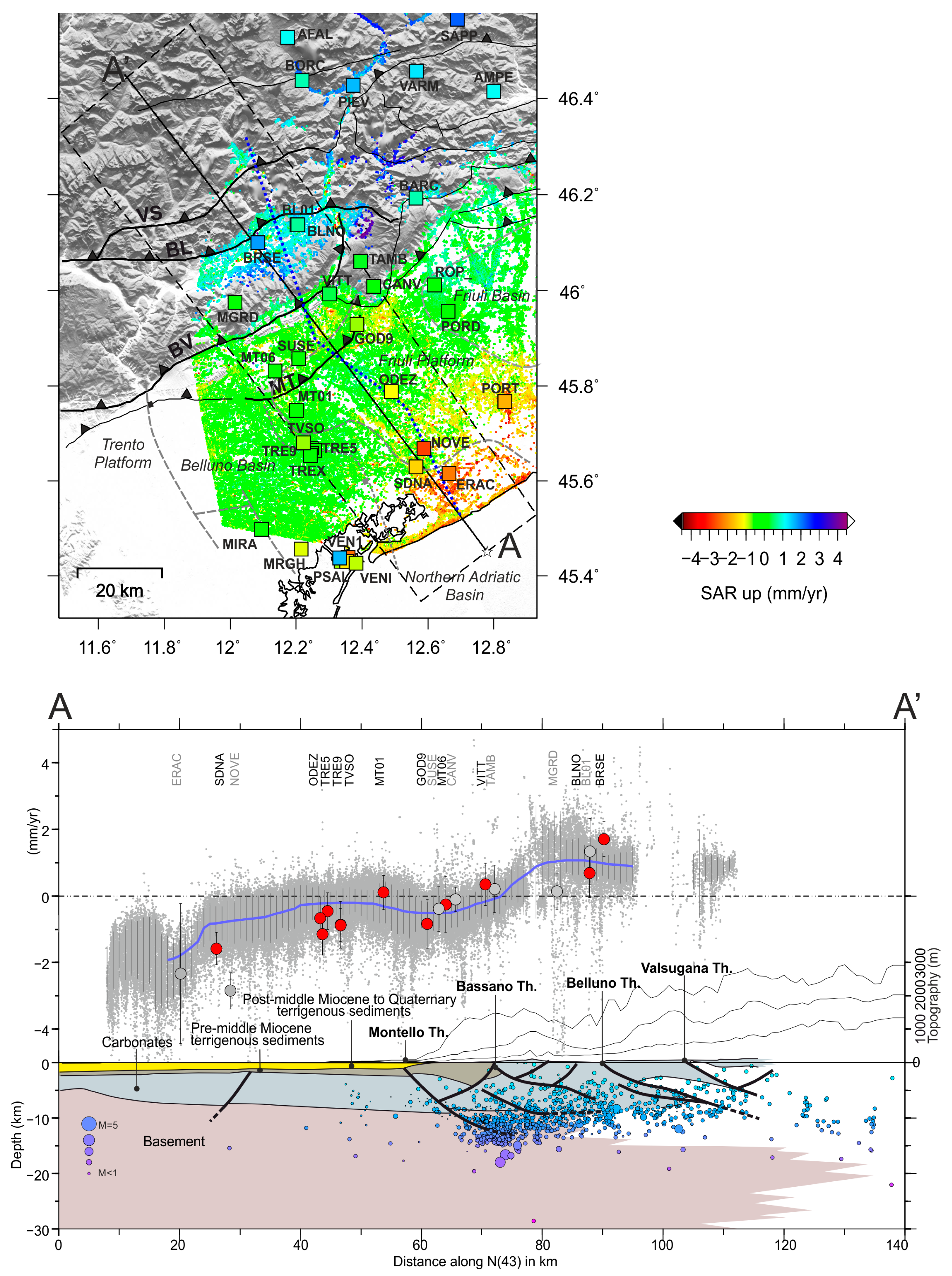
• A positive vertical gradient of 1 mm/yr is observed between the Montello and the Prealps due to strain accumulation of the deepest portion of the thrusts. Specifically, we suggested the Bassano-Valdobbiandene thrust as the main one responsible for the interseismic signal detected in the area.
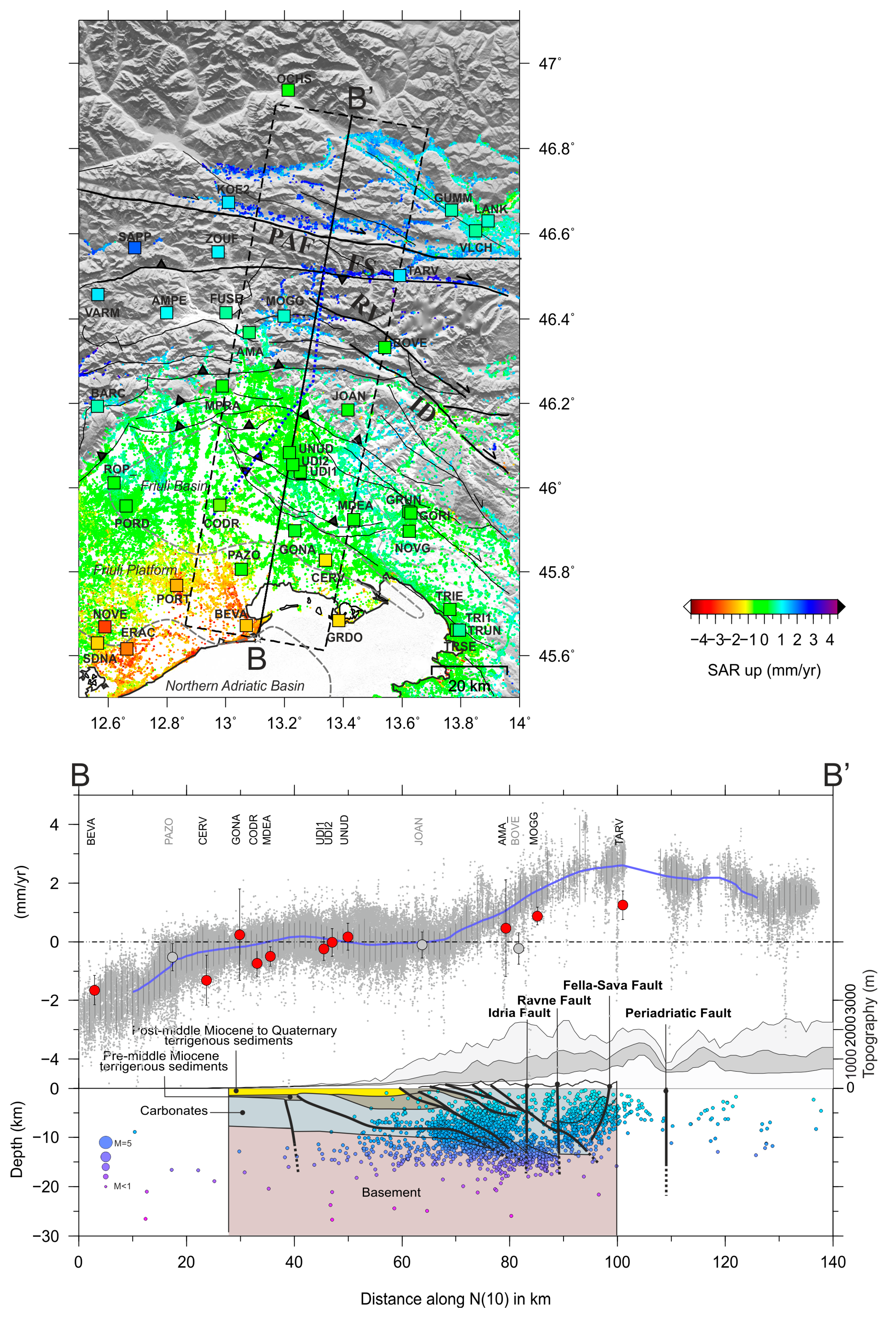
• The eastward (1 mm/yr) and upward (1–2 mm/yr) interseismic signals are accommodated by the Friulian Alpine-Dinaric faults (i.e., thrusts and strike-slip faults) in the area.
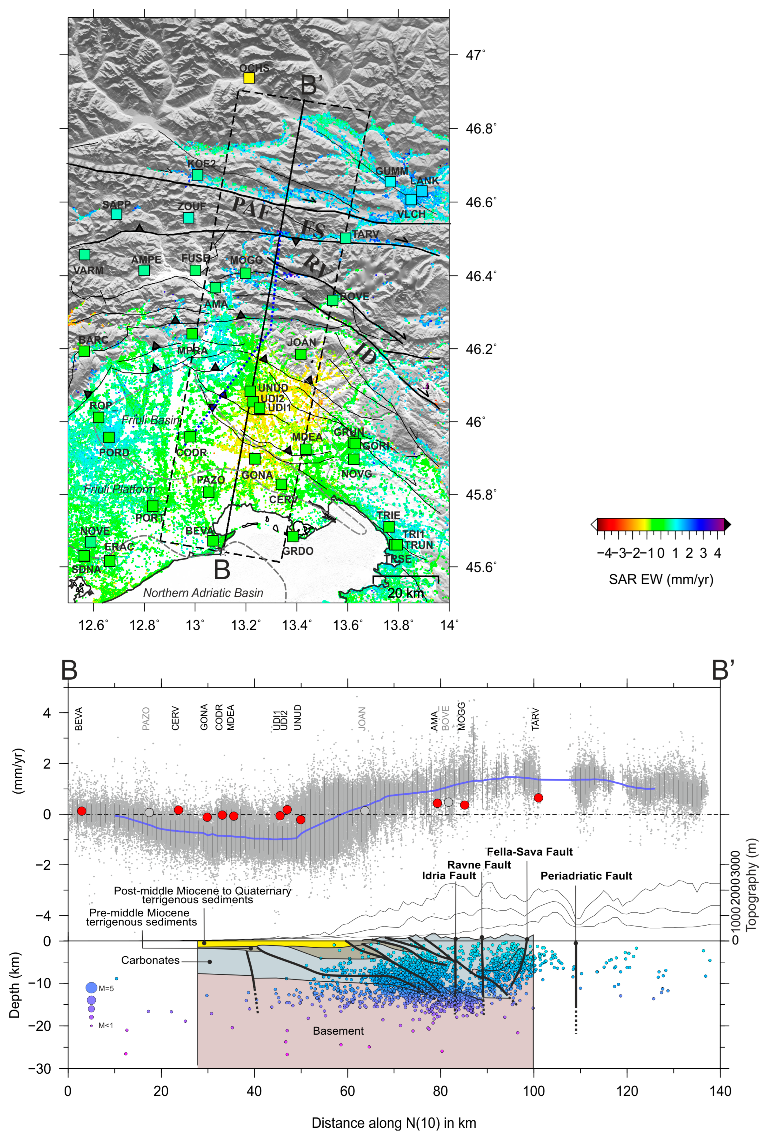
• The westward signal of 1 mm/yr recorded near Udine might be related to transcurrent-transpressive systems and buried thrusts, although further investigations and analysis are required.
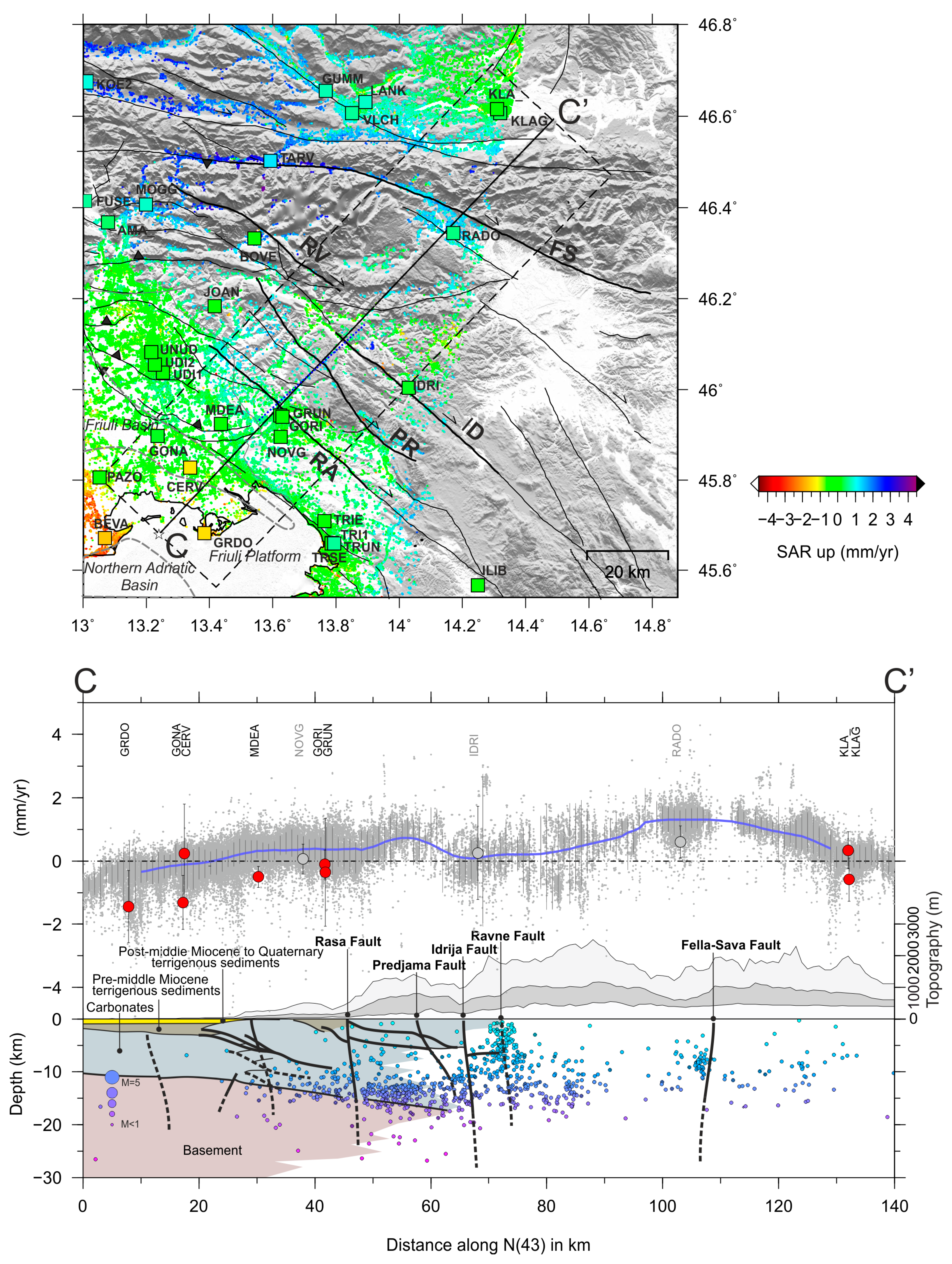
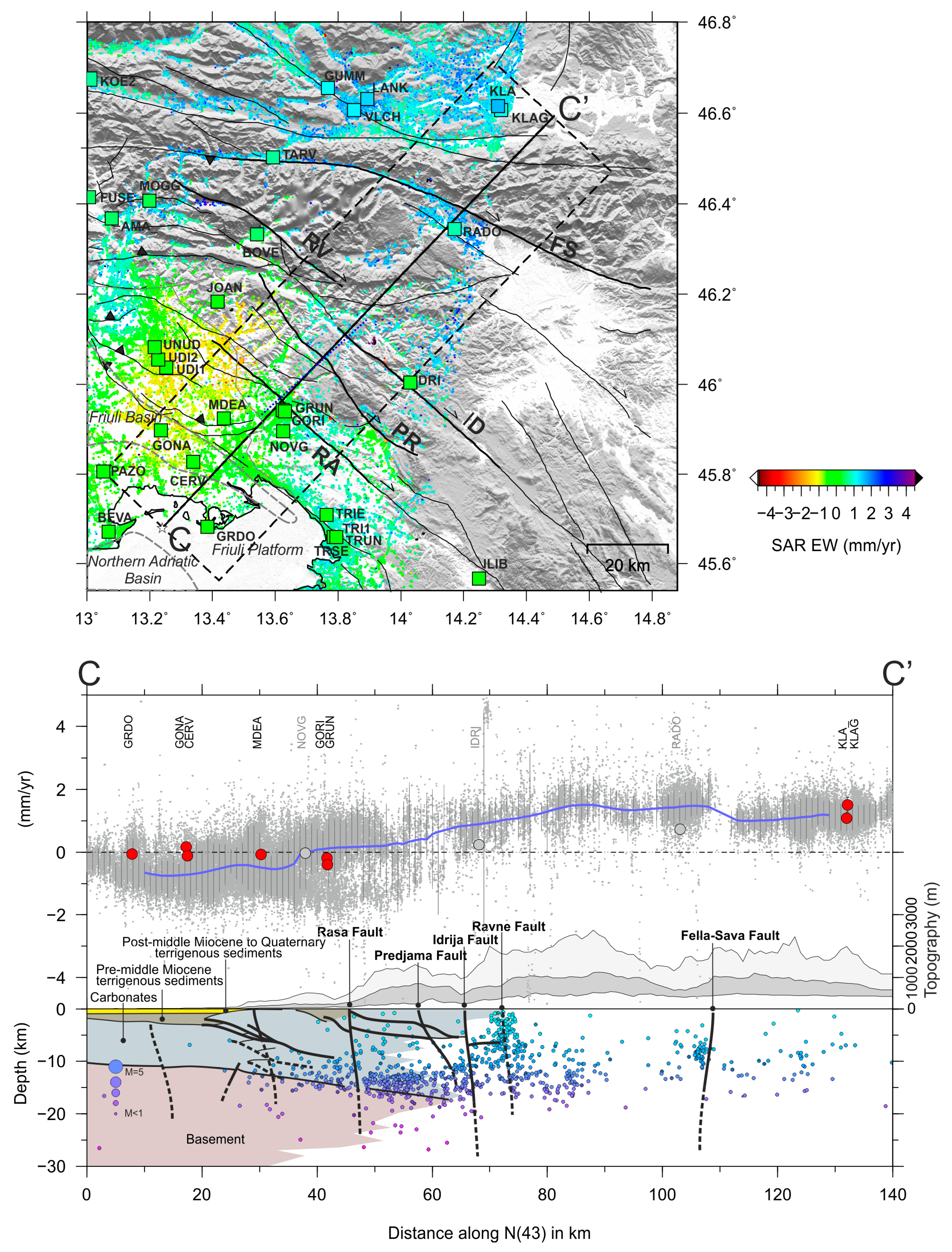
• The velocity profiles traced across the Dinaric dextral strike-slip faults show an uplift and an eastward motion (about 1 mm/yr) that can be attributed to the tectonic activity of the Raša, Predjama, and Idrija faults.

Regarding non-tectonic signals, we observe diffuse subsidence mainly on the Venetian-Friulian plain and along the coasts (0.5–2 mm/yr), confirming a strong correlation with the geological setting of the area. Strong local subsidence signals can also be identified (i.e., Portogruaro) due to several natural and anthropogenic causes that induce differential subsidence in the areas.

Our study provides a detailed view of the regional deformation processes in the study area, mainly focused on interseismic and subsidence signals. However, further analysis should be conducted to deepen our knowledge of the ongoing processes. Time-series analysis and correlation with ancillary data (e.g., temperature, extraction of fluids, and groundwater variations) are necessary to improve the understanding of their effects and their evolution in time and space. In addition, fault modeling (i.e., 2D and 3D models) is fundamental to defining the geometric and kinematic parameters of active faults and deepening our knowledge of their seismogenic potential (i.e., estimation of locking depths and slip rates).

References

1. Grandin, R.; Doin, M.-P.; Bollinger, L.; Pinel-Puysségur, B.; Ducret, G.; Jolivet, R.; Sapkota, S.N. Long-term growth of the Himalaya inferred from interseismic InSAR measurement. Geology 2012, 40, 1059–1062. [Google Scholar] [CrossRef] [Green Version]
2. Pezzo, G.; Tolomei, C.; Atzori, S.; Salvi, S.; Shabanian, E.; Bellier, O.; Farbod, Y. New kinematic constraints of the western Doruneh fault, northeastern Iran, from interseismic deformation analysis. Geophys. J. Int. 2012, 190, 622–628. [Google Scholar] [CrossRef] [Green Version]
3. Karimzadeh, S.; Cakir, Z.; Osmanoğlu, B.; Schmalzle, G.; Miyajima, M.; Amiraslanzadeh, R.; Djamour, Y. Interseismic strain accumulation across the North Tabriz Fault (NW Iran) deduced from InSAR time series. J. Geodyn. 2013, 66, 53–58. [Google Scholar] [CrossRef]
4. Liu, C.; Ji, L.; Zhu, L.; Zhao, C. InSAR-Constrained Interseismic Deformation and Potential Seismogenic Asperities on the Altyn Tagh. Remote Sens. 2018, 10, 943. [Google Scholar] [CrossRef] [Green Version]
5. Fialko, Y. Interseismic strain accumulation and the earthquake potential on the southern San Andreas fault system. Nature 2006, 441, 968–971. [Google Scholar] [CrossRef] [PubMed] [Green Version]
6. Tong, X.; Sandwell, D.T.; Smith-Konter, B. High-resolution interseismic velocity data along the San Andreas Fault from GPS and InSAR. J. Geophys. Res. Solid Earth 2013, 118, 369–389. [Google Scholar] [CrossRef] [Green Version]
7. Chaussard, E.; Johnson, C.W.; Fattahi, H.; Bürgmann, R. Potential and limits of InSAR to characterize interseismic deformation independently of GPS data: Application to the southern San Andreas Fault system. Geochem. Geophys. Geosyst. 2016, 17, 1214–1229. [Google Scholar] [CrossRef] [Green Version]
8. Wright, T.; Parsons, B.; Fielding, E. Measurement of interseismic strain accumulation across the North Anatolian Fault by satellite radar interferometry. Geophys. Res. Lett. 2001, 28, 2117–2120. [Google Scholar] [CrossRef]
9. Walters, R.J.; Holley, R.J.; Parsons, B.; Wright, T.J. Interseismic strain accumulation across the North Anatolian Fault from Envisat InSAR measurements. Geophys. Res. Lett. 2011, 38, L05303. [Google Scholar] [CrossRef] [Green Version]
10. Hussain, E.; Hooper, A.; Wright, T.J.; Walters, R.J.; Bekaert, D.P.S. Interseismic strain accumulation across the central North Anatolian Fault from iteratively unwrapped InSAR measurements. J. Geophys. Res. Solid Earth 2016, 121, 9000–9019. [Google Scholar] [CrossRef] [Green Version]
11. Weiss, J.R.; Walters, R.J.; Morishita, Y.; Wright, T.J.; Lazecky, M.; Wang, H.; Hussain, E.; Hooper, A.J.; Elliott, J.R.; Rollins, C.; et al. High-Resolution Surface Velocities and Strain for Anatolia From Sentinel-1 InSAR and GNSS Data. Geophys. Res. Lett. 2020, 47, e2020GL087376. [Google Scholar] [CrossRef]
12. Cheloni, D.; D’Agostino, N.; Selvaggi, G. Interseismic coupling, seismic potential, and earthquake recurrence on the southern front of the Eastern Alps (NE Italy). J. Geophys. Res. Solid Earth 2014, 119, 4448–4468. [Google Scholar] [CrossRef]
13. Pezzo, G.; Merryman Boncori, J.P.; Visini, F.; Carafa, M.M.C.; Devoti, R.; Atzori, S.; Kastelic, V.; Berardino, P.; Fornaro, G.; Riguzzi, F.; et al. Interseismic Ground Velocities of the Central Apennines from GPS and SAR Measurements and Their Contribution to Seismic hazard Modelling: Preliminary Results of the ESA CHARMING Project. Misc. INGV 2015.
14. Pezzo, G.; Petracchini, L.; Devoti, R.; Maffucci, R.; Anderlini, L.; Antoncecchi, I.; Billi, A.; Carminati, E.; Ciccone, F.; Cuffaro, M.; et al. Active Fold-Thrust Belt to Foreland Transition in Northern Adria, Italy, Tracked by Seismic Reflection Profiles and GPS Offshore Data. Tectonics 2020, 39, e2020TC006425. [Google Scholar] [CrossRef]
15. Serpelloni, E.; Vannucci, G.; Anderlini, L.; Bennett, R.A. Kinematics, seismotectonics and seismic potential of the eastern sector of the European Alps from GPS and seismic deformation data. Tectonophysics 2016, 688, 157–181. [Google Scholar] [CrossRef]
16. Anderlini, L.; Serpelloni, E.; Tolomei, C.; Marco De Martini, P.; Pezzo, G.; Gualandi, A.; Spada, G. New insights into active tectonics and seismogenic potential of the Italian Southern Alps from vertical geodetic velocities. Solid Earth 2020, 11, 1681–1698. [Google Scholar] [CrossRef]
17. Teatini, P.; Tosi, L.; Strozzi, T.; Carbognin, L.; Wegmüller, U.; Rizzetto, F. Mapping regional land displacements in the Venice coastland by an integrated monitoring system. Remote Sens. Environ. 2005, 98, 403–413. [Google Scholar] [CrossRef]
18. Tosi, L.; Teatini, P.; Strozzi, T.; Carbognin, L.; Brancolini, G.; Rizzetto, F. Ground surface dynamics in the northern Adriatic coastland over the last two decades. Rend. Lince 2010, 21, 115–129. [Google Scholar] [CrossRef]
19. Tosi, L.; Teatini, P.; Strozzi, T. Natural versus anthropogenic subsidence of Venice. Sci. Rep. 2013, 3, 2710. [Google Scholar] [CrossRef] [PubMed] [Green Version]
20. Osmanoğlu, B.; Dixon, T.H.; Wdowinski, S.; Cabral-Cano, E.; Jiang, Y. Mexico City subsidence observed with persistent scatterer InSAR. Int. J. Appl. Earth Obs. Geoinf. 2011, 13, 1–12. [Google Scholar] [CrossRef]
21. Da Lio, C.; Tosi, L. Science of the Total Environment Land subsidence in the Friuli Venezia Giulia coastal plain, Italy: 1992–2010 results from SAR-based interferometry. Sci. Total Environ. 2018, 633, 752–764. [Google Scholar] [CrossRef]
22. Del Soldato, M.; Farolfi, G.; Rosi, A.; Raspini, F.; Casagli, N. Subsidence Evolution of the Firenze–Prato–Pistoia Plain (Central Italy) Combining PSI and GNSS Data. Remote Sens. 2018, 10, 1146. [Google Scholar] [CrossRef] [Green Version]
23. Polcari, M.; Albano, M.; Montuori, A.; Bignami, C.; Tolomei, C.; Pezzo, G.; Falcone, S.; La Piana, C.; Doumaz, F.; Salvi, S.; et al. InSAR Monitoring of Italian Coastline Revealing Natural and Anthropogenic Ground Deformation Phenomena and Future Perspectives. Sustainability 2018, 10, 3152. [Google Scholar] [CrossRef] [Green Version]
24. Farolfi, G.; Bianchini, S.; Casagli, N. Integration of GNSS and Satellite InSAR Data: Derivation of Fine-Scale Vertical Surface Motion Maps of Po Plain, Northern Apennines, and Southern Alps, Italy. IEEE Trans. Geosci. Remote Sens. 2019, 57, 319–328. [Google Scholar] [CrossRef]
25. Farolfi, G.; Del Soldato, M.; Bianchini, S.; Casagli, N. A procedure to use GNSS data to calibrate satellite PSI data for the study of subsidence: An example from the north-western Adriatic coast (Italy). Eur. J. Remote Sens. 2019, 52, 54–63. [Google Scholar] [CrossRef] [Green Version]
26. Floris, M.; Fontana, A.; Tessari, G.; Mulè, M. Subsidence Zonation Through Satellite Interferometry in Coastal Plain Environments of NE Italy: A Possible Tool for Geological and Geomorphological Mapping in Urban Areas. Remote Sens. 2019, 11, 165. [Google Scholar] [CrossRef] [Green Version]
27. Žibret, G.; Komac, M.; Jemec, M. PSInSAR displacements related to soil creep and rainfall intensities in the Alpine foreland of western Slovenia. Geomorphology 2012, 175–176, 107–114. [Google Scholar] [CrossRef]
28. Komac, M.; Holley, R.; Mahapatra, P.; van der Marel, H.; Bavec, M. Coupling of GPS/GNSS and radar interferometric data for a 3D surface displacement monitoring of landslides. Landslides 2015, 12, 241–257. [Google Scholar] [CrossRef]
29. Notti, D.; Calò, F.; Cigna, F.; Manunta, M.; Herrera, G.; Berti, M.; Meisina, C.; Tapete, D.; Zucca, F. A User-Oriented Methodology for DInSAR Time Series Analysis and Interpretation: Landslides and Subsidence Case Studies. Pure Appl. Geophys. 2015, 172, 3081–3105. [Google Scholar] [CrossRef] [Green Version]
30. Aslan, G.; Foumelis, M.; Raucoules, D.; De Michele, M.; Bernardie, S.; Cakir, Z. Landslide Mapping and Monitoring Using Persistent Scatterer Interferometry (PSI) Technique in the French Alps. Remote Sens. 2020, 12, 1305. [Google Scholar] [CrossRef] [Green Version]
31. Busetti, A.; Calligaris, C.; Forte, E.; Areggi, G.; Mocnik, A.; Zini, L. Non-Invasive Methodological Approach to Detect and Characterize High-Risk Sinkholes in Urban Cover Evaporite Karst: Integrated Reflection Seismics, PS-InSAR, Leveling, 3D-GPR and Ancillary Data. A NE Italian Case Study. Remote Sens. 2020, 12, 3814. [Google Scholar] [CrossRef]
32. Hooper, A.; Segall, P.; Zebker, H. Persistent scatterer interferometric synthetic aperture radar for crustal deformation analysis, with application to Volcán Alcedo, Galápagos. J. Geophys. Res. Atmos. 2007, 112, 1–21. [Google Scholar] [CrossRef] [Green Version]
33. Pezzo, G.; Palano, M.; Tolomei, C.; De Gori, P.; Calcaterra, S.; Gambino, P.; Chiarabba, C. Flank sliding: A valve and a sentinel for paroxysmal eruptions and magma ascent at Mount Etna, Italy. Geology 2020, 48, 1077–1082. [Google Scholar] [CrossRef]
34. Beccaro, L.; Tolomei, C.; Gianardi, R.; Sepe, V.; Bisson, M.; Colini, L.; De Ritis, R.; Spinetti, C. Multitemporal and Multisensor InSAR Analysis for Ground Displacement Field Assessment at Ischia Volcanic Island (Italy). Remote Sens. 2021, 13, 4253. [Google Scholar] [CrossRef]
35. Perski, Z.; Hanssen, R.; Wojcik, A.; Wojciechowski, T. InSAR analyses of terrain deformation near the Wieliczka Salt Mine, Poland. Eng. Geol. 2009, 106, 58–67. [Google Scholar] [CrossRef]
36. Klemm, H.; Quseimi, I.; Novali, F.; Ferretti, A.; Tamburini, A. Monitoring horizontal and vertical surface deformation over a hydrocarbon reservoir by PSInSAR. First Break. 2010, 28, 29–37. [Google Scholar] [CrossRef] [Green Version]
37. Ab Latip, A.S.; Matori, A.; Aobpaet, A.; Din, A.H.M. Monitoring of offshore platform deformation with stanford method of Persistent Scatterer (StaMPS). Int. Conf. Sp. Sci. Commun. Iconsp. 2015, 2015, 79–83. [Google Scholar] [CrossRef]
38. Gama, F.F.; Mura, J.G.; Paradella, W.R.; De Oliveira, C.G. Deformations Prior to the Brumadinho Dam Collapse Revealed by Sentinel-1 InSAR Data Using SBAS and PSI Techniques. Remote Sens. 2020, 12, 3664. [Google Scholar] [CrossRef]
39. Kumar Maurya, V.; Dwivedi, R.; Ranjan Martha, T. Site scale landslide deformation and strain analysis using MT-InSAR and GNSS approach—A case study. Adv. Space Res. 2022, 70, 3932–3947. [Google Scholar] [CrossRef]
40. Yalvac, S. Validating InSAR-SBAS results by means of different GNSS analysis techniques in medium- and high-grade deformation areas. Environ. Monit. Assess. 2020, 192, 120. [Google Scholar] [CrossRef]
41. Li, Y. Analysis of GAMIT/GLOBK in high-precision GNSS data processing for crustal deformation. Earthq. Res. Adv. 2021, 1, 100028. [Google Scholar] [CrossRef]
42. Nof, R.N.; Abelson, M.; Raz, E.; Magen, Y.; Atzori, S.; Salvi, S.; Baer, G. SAR Interferometry for Sinkhole Early Warning and Susceptibility Assessment along the Dead Sea, Israel. Remote Sens. 2019, 11, 89. [Google Scholar] [CrossRef] [Green Version]
43. Li, Y.; Jiang, W.; Zhang, J.; Li, B.; Yan, R.; Wang, X. Sentinel-1 SAR-Based coseismic deformation monitoring service for rapid geodetic imaging of global earthquakes. Nat. Hazards Res. 2021, 1, 11–19. [Google Scholar] [CrossRef]
44. Castellarin, A.; Vai, G.B.; Cantelli, L. The Alpine evolution of the Southern Alps around the Giudicarie faults: A Late Cretaceous to Early Eocene transfer zone. Tectonophysics 2006, 414, 203–223. [Google Scholar] [CrossRef]
45. Aoudia, A.; Saraò, A.; Bukchin, B.; Suhadolc, P. The 1976 Friuli (NE Italy) thrust faulting earthquake: A reappraisal 23 years later. Geophys. Res. Lett. 2000, 27, 577–580. [Google Scholar] [CrossRef]
46. Pondrelli, S.; Ekström, G.; Morelli, A. Seismotectonic re-evaluation of the 1976 Friuli, Italy, seismic sequence. J. Seism. 2001, 5, 73–83. [Google Scholar] [CrossRef]
47. Carulli, G.B.; Slejko, D. The 1976 Friuli, Italy, Earthquake. G. Geol. Appl. 2005, 1, 147–156. [Google Scholar] [CrossRef]
48. Anselmi, M.; Govoni, A.; De Gori, P.; Chiarabba, C. Seismicity and velocity structures along the south-Alpine thrust front of the Venetian Alps (NE-Italy). Tectonophysics 2011, 513, 37–48. [Google Scholar] [CrossRef]
49. Danesi, S.; Pondrelli, S.; Salimbeni, S.; Cavaliere, A.; Serpelloni, E.; Danecek, P.; Lovati, S.; Massa, M. Active deformation and seismicity in the Southern Alps (Italy): The Montello hill as a case study. Tectonophysics 2015, 653, 95–108. [Google Scholar] [CrossRef]
50. Bressan, G.; Ponton, M.; Rossi, G.; Urban, S. Spatial organization of seismicity and fracture pattern in NE Italy and W Slovenia. J. Seism. 2016, 20, 511–534. [Google Scholar] [CrossRef] [PubMed] [Green Version]
51. Rovida, A.; Locati, M.; Camassi, R.; Lolli, B.; Gasperini, P. The Italian earthquake catalogue CPTI15. Bull. Earthq. Eng. 2020, 18, 2953–2984. [Google Scholar] [CrossRef]
52. Carbognin, L.; Teatini, P.; Tomasin, A.; Tosi, L. Global change and relative sea level rise at Venice: What impact in term of flooding. Clim. Dyn. 2009, 35, 1055–1063. [Google Scholar] [CrossRef]
53. D’Agostino, N.; Cheloni, D.; Mantenuto, S.; Selvaggi, G.; Michelini, A.; Zuliani, D. Strain accumulation in the southern Alps (NE Italy) and deformation at the northeastern boundary of Adria observed by CGPS measurements. Geophys. Res. Lett. 2005, 32, 1–4. [Google Scholar] [CrossRef]
54. Vrabec, M.; Prešeren, P.P.; Stopar, B. GPS study (1996–2002) of active deformation along the Periadriatic fault system in northeastern Slovenia: Tectonic model. Geol. Carpathica 2006, 57, 57–65. [Google Scholar]
55. Bechtold, M.; Battaglia, M.; Tanner, D.C.; Zuliani, D. Constraints on the active tectonics of the Friuli/NW Slovenia area from CGPS measurements and three-dimensional kinematic modeling. J. Geophys. Res. Solid Earth. 2009, 114, B03408. [Google Scholar] [CrossRef] [Green Version]
56. Moulin, A.; Benedetti, L.; Rizza, M.; Jamšek Rupnik, P.; Gosar, A.; Bourlès, D.; Keddadouche, K.; Aumaître, G.; Arnold, M.; Guillou, V.; et al. The Dinaric fault system: Large-scale structure, rates of slip, and Plio-Pleistocene evolution of the transpressive northeastern boundary of the Adria microplate. Tectonics 2016, 35, 2258–2292. [Google Scholar] [CrossRef] [Green Version]
57. Rossi, G.; Zuliani, D.; Fabris, P. Tectonophysics Long-term GNSS measurements from the northern Adria microplate reveal fault-induced fluid mobilization. Tectonophysics 2016, 690, 142–159. [Google Scholar] [CrossRef]
58. Rossi, G.; Fabris, P.; Zuliani, D. Overpressure and Fluid Diffusion Causing Non-hydrological Transient GNSS Displacements. Pure Appl. Geophys. 2018, 175, 1869–1888. [Google Scholar] [CrossRef]
59. Rossi, G.; Pastorutti, A.; Nagy, I.; Braitenberg, C.; Parolai, S. Recurrence of Fault Valve Behavior in a Continental Collision Area: Evidence From Tilt/Strain Measurements in Northern Adria. Front. Earth Sci. 2021, 9, 641416. [Google Scholar] [CrossRef]
60. Stocchi, P.; Spada, G.; Cianetti, S. Isostatic rebound following the Alpine deglaciation: Impact on the sea level variations and vertical movements in the Mediterranean region. Geophys. J. Int. 2005, 162, 137–147. [Google Scholar] [CrossRef] [Green Version]
61. Devoti, R.; Zuliani, D.; Braitenberg, C.; Fabris, P.; Grillo, B. Hydrologically induced slope deformations detected by GPS and clinometric surveys in the Cansiglio Plateau, southern Alps. Earth Planet. Sci. Lett. 2015, 419, 134–142. [Google Scholar] [CrossRef]
62. Serpelloni, E.; Pintori, F.; Gualandi, A.; Scoccimarro, E.; Cavaliere, A.; Anderlini, L.; Belardinelli, M.E.; Todesco, M. Journal of Geophysical Research: Solid Earth Hydrologically Induced Karst Deformation: Insights From GPS Measurements in the Adria-Eurasia Plate Boundary Zone. J. Geophys. Res. Solid Earth 2018, 123, 4413–4430. [Google Scholar] [CrossRef]
63. Pintori, F.; Serpelloni, E.; Longuevergne, L.; Garcia, A.; Faenza, L.; D’Alberto, L.; Gualandi, A.; Belardinelli, M.E. Mechanical Response of Shallow Crust to Groundwater Storage Variations: Inferences From Deformation and Seismic Observations in the Eastern Southern Alps, Italy. J. Geophys. Res. Solid Earth 2021, 126, e2020JB020586. [Google Scholar] [CrossRef]
64. Bock, Y.; Wdowinski, S.; Ferretti, A.; Novali, F.; Fumagalli, A. Recent subsidence of the Venice Lagoon from continuous GPS and interferometric synthetic aperture radar. Geochem. Geophys. Geosyst. 2012, 13, Q03023. [Google Scholar] [CrossRef]
65. Serpelloni, E.; Faccenna, C.; Spada, G.; Dong, D.; Williams, S.D.P. Vertical GPS ground motion rates in the Euro-Mediterranean region: New evidence of velocity gradients at different spatial scales along the Nubia-Eurasia plate boundary. J. Geophys. Res. Solid Earth 2013, 118, 6003–6024. [Google Scholar] [CrossRef] [Green Version]
66. Vecchio, A.; Anzidei, M.; Serpelloni, E.; Florindo, F. Natural Variability and Vertical Land Motion Contributions in the Mediterranean Sea-Level Records over the Last Two Centuries and Projections for 2100. Water 2019, 11, 1480. [Google Scholar] [CrossRef] [Green Version]
67. Asch, K. IGME 5000:1:5 Million International Geological Map of Europe and Adjacent Areas -final version for the internet- BGR, Hannover. 2005. Available online: https://services.bgr.de/geologie/igme5000 (accessed on 15 March 2023).
68. Nicolich, R.; Della Vedova, B.; Giustiniani, M.; Fantoni, R. Carta del sottosuolo Della Pianura Friulana. 2004. Available online: https://www.regione.fvg.it/rafvg/export/sites/default/RAFVG/ambiente-territorio/geologia/FOGLIA16/allegati/note_illustrative.pdf (accessed on 15 March 2023).
69. Fantoni, R.; Franciosi, R. Tectono-sedimentary setting of the Po Plain and Adriatic foreland. Rend. Fis. Acc. Lincei. 2010, 21, 197–209. [Google Scholar] [CrossRef]
70. Masetti, D.; Fantoni, R.; Romano, R.; Sartorio, D.; Trevisani, E. Tectonostratigraphic evolution of the Jurassic extensional basins of the eastern southern Alps and Adriatic foreland based on an integrated study of surface and subsurface data. Am. Assoc. Pet. Geol. Bull. 2012, 96, 2065–2089. [Google Scholar] [CrossRef]
71. Mellere, D.; Stefani, C.; Angevine, C. Polyphase Tectonics through subsidence analysis: The Oligo-Miocene Venetian and Friuli Basin, north-east Italy. Basin Res. 2000, 12, 159–182. [Google Scholar] [CrossRef]
72. Toscani, G.; Marchesini, A.; Barbieri, C.; Di Giulio, A.; Fantoni, R.; Mancin, N.; Zanferrari, A. The Friulian-Venetian Basin I: Architecture and sediment flux into a shared foreland basin. Ital. J. Geosci. 2016, 135, 444–459. [Google Scholar] [CrossRef]
73. Bosellini, A.; Masetti, D.; Sarti, M. A Jurassic “Tongue of the Ocean” infilled with oolitic sands: The Belluno Trough, Venetian Alps, Italy. Mar. Geol. 1981, 44, 59–95. [Google Scholar] [CrossRef]
74. Placer, L.; Vrabec, M.; Celarc, B. The bases for understanding of the NW Dinarides and Istria Peninsula tectonics. Geologija 2010, 53, 55–86. [Google Scholar] [CrossRef]
75. Doglioni, C.; Bosellini, A. Eoalpine and mesoalpine tectonics in the Southern Alps. Geol. Rundsch. 1987, 76, 735–754. [Google Scholar] [CrossRef]
76. Castellarin, A.; Cantelli, L. Neo-Alpine evolution of the Southern Eastern Alps. J. Geodyn. 2000, 30, 251–274. [Google Scholar] [CrossRef]
77. Bressan, G.; Bragato, P.L.; Venturini, C. Stress and Strain Tensors Based on Focal Mechanisms in the Seismotectonic Framework of the Friuli-Venezia Giulia Region (Northeastern Italy). Bull. Seism. Soc. Am. 2003, 93, 1280–1297. [Google Scholar] [CrossRef]
78. Vrabec, M.; Fodor, L. Late Cenozoic tectonics of Slovenia: Structural styles at the northeastern corner of the Adriatic microplate. In The Adria Microplate: GPS Geodesy, Tectonics and Hazards; Springer: Dordrecht, The Netherlands, 2006; pp. 151–168. [Google Scholar] [CrossRef]
79. Galadini, F.; Poli, M.E.; Zanferrari, A. Seismogenic sources potentially responsible for earthquakes with M≥ 6 in the eastern Southern Alps (Thiene-Udine sector, NE Italy). Geophys. J. Int. 2005, 161, 739–762. [Google Scholar] [CrossRef] [Green Version]
80. Burrato, P.; Poli, M.E.; Vannoli, P.; Zanferrari, A.; Basili, R.; Galadini, F. Sources of Mw 5+ earthquakes in northeastern Italy and western Slovenia: An updated view based on geological and seismological evidence. Tectonophysics 2008, 453, 157–176. [Google Scholar] [CrossRef]
81. Bressan, G.; Barnaba, C.; Bragato, P.; Ponton, M.; Restivo, A. Revised seismotectonic model of NE Italy and W Slovenia based on focal mechanism inversion. J. Seism. 2018, 22, 1563–1578. [Google Scholar] [CrossRef]
82. Atanackov, J.; Jamšek Rupnik, P.; Jež, J.; Celarc, B.; Novak, M.; Milanič, B.; Markelj, A.; Bavec, M.; Kastelic, V. Database of Active Faults in Slovenia: Compiling a New Active Fault Database at the Junction Between the Alps, the Dinarides and the Pannonian Basin Tectonic Domains. Front. Earth Sci. 2021, 9, 604388. [Google Scholar] [CrossRef]
83. DISS Working Group Database of Individual Seismogenic Sources (DISS), Version 3.3.0: A Compilation of Potential Sources for Earthquakes Larger than M 5.5 in Italy and Surrounding Areas. 2021. Available online: https://diss.ingv.it/ (accessed on 15 March 2023).
84. Bajc, J.; Aoudia, A.; Saraò, A.; Suhadolc, P. The 1998 Bovec-Krn Mountain (Slovenia) Earthquake Sequence. Geophys. Res. Lett. 2001, 28, 1839–1842. [Google Scholar] [CrossRef]
85. Poli, M.E.; Peruzza, L.; Rebez, A.; Slejko, D. New seismotectonic evidence from the analysis of the 1976–1977 and 1977–1999 seismicity in Friuli (NE Italy). Boll. Geofis. Teor. Appl. 2002, 43, 53–78. [Google Scholar]
86. Bressan, G.; Gentile, G.F.; Perniola, B.; Urban, S. The 1998 and 2004 Bovec-Krn (Slovenia) seismic sequences: Aftershock pattern, focal mechanisms and static stress changes. Geophys. J. Int. 2009, 179, 231–253. [Google Scholar] [CrossRef] [Green Version]
87. Poli, M.E.; Zanferrari, A. The Seismogenic Sources of the 1976 Friuli Earthquakes: A new seismotectonic model for the Friuli area. Boll. Geofis. Teor. Appl. 2018, 59, 463–480. [Google Scholar] [CrossRef]
88. Tosi, L.; Teatini, P.; Carbognin, L.; Brancolini, G. Using high resolution data to reveal depth-dependent mechanisms that drive land subsidence: The Venice coast, Italy. Tectonophysics 2009, 474, 271–284. [Google Scholar] [CrossRef]
89. Brambati, A.; Carbognin, L.; Quaia, T.; Teatini, P.; Tosi, L. The Lagoon of Venice: Geological setting, evolution and land subsidence. Episodes 2003, 26, 264–265. [Google Scholar] [CrossRef]
90. De Zan, F.; Guarnieri, A.M. TOPSAR: Terrain Observation by Progressive Scans. IEEE Trans. Geosci. Remote Sens. 2006, 44, 2352–2360. [Google Scholar] [CrossRef]
91. Torres, R.; Snoeij, P.; Geudtner, D.; Bibby, D.; Davidson, M.; Attema, E.; Potin, P.; Rommen, B.; Floury, N.; Brown, M.; et al. GMES Sentinel-1 mission. Remote Sens. Environ. 2012, 120, 9–24. [Google Scholar] [CrossRef]
92. Crosetto, M.; Monserrat, O.; Cuevas-González, M.; Devanthéry, N.; Crippa, B. Persistent Scatterer Interferometry: A review. ISPRS J. Photogramm. Remote Sens. 2016, 115, 78–89. [Google Scholar] [CrossRef] [Green Version]
93. Foumelis, M.; Blasco, J.M.D.; Desnos, Y.L.; Engdahl, M.; Fernández, D.; Veci, L.; Lu, J.; Wong, C. ESA SNAP—Stamps integrated processing for Sentinel-1 persistent scatterer interferometry. In Proceedings of the 2018 IEEE International Geoscience and Remote Sensing Symposium, Valencia, Spain, 22–27 July 2018; pp. 1364–1367. [Google Scholar] [CrossRef]
94. Chen, C.W.; Zebker, H.A. Phase unwrapping for large SAR interferograms: Statistical segmentation and generalized network models. IEEE Trans. Geosci. Remote Sens. 2002, 40, 1709–1719. [Google Scholar] [CrossRef] [Green Version]
95. Goldstein, R.M.; Werner, C.L. Radar interferogram filtering for geophysical applications. Geophys. Res. Lett. 1998, 25, 4035–4038. [Google Scholar] [CrossRef] [Green Version]
96. Ferretti, A.; Prati, C.; Rocca, F. Nonlinear Subsidence Rate Estimation Using permanent scatterers in differential SAR interferometry. IEEE Trans. Geosci. Remote Sens. 2000, 38, 2202–2212. [Google Scholar] [CrossRef] [Green Version]
97. Ferretti, A.; Prati, C.; Rocca, F. Permanent scatters in SAR interferometry. IEEE Trans. Geosci. Remote Sens. 2001, 39, 8–20. [Google Scholar] [CrossRef]
98. Berardino, P.; Fornaro, G.; Lanari, R.; Sansosti, E. A new algorithm for surface deformation monitoring based on small baseline differential SAR interferograms. IEEE Trans. Geosci. Remote Sens. 2002, 40, 2375–2383. [Google Scholar] [CrossRef] [Green Version]
99. Doin, M.-P.; Lasserre, C.; Peltzer, G.; Cavalié, O.; Doubre, C. Corrections of stratified tropospheric delays in SAR interferometry: Validation with global atmospheric models. J. Appl. Geophys. 2009, 69, 35–50. [Google Scholar] [CrossRef]
100. Hooper, A.; Bekaert, D.; Spaans, K.; Arıkan, M. Recent advances in SAR interferometry time series analysis for measuring crustal deformation. Tectonophysics 2012, 514–517, 1–13. [Google Scholar] [CrossRef]
101. Farolfi, G.; Piombino, A.; Catani, F. Fusion of GNSS and Satellite Radar Interferometry: Determination of 3D Fine-Scale Map of Present-Day Surface Displacements in Italy as Expressions of Geodynamic Processes. Remote Sens. 2019, 11, 394. [Google Scholar] [CrossRef] [Green Version]
102. Del Soldato, M.; Confuorto, P.; Bianchini, S.; Sbarra, P.; Casagli, N. Review of Works Combining GNSS and InSAR in Europe. Remote Sens. 2021, 13, 1684. [Google Scholar] [CrossRef]
103. Cigna, F.; Ramírez, R.E.; Tapete, D. Accuracy of Sentinel-1 PSI and SBAS InSAR Displacement Velocities against GNSS and Geodetic Leveling Monitoring Data. Remote Sens. 2021, 13, 4800. [Google Scholar] [CrossRef]
104. Serpelloni, E.; Cavaliere, A.; Martelli, L.; Pintori, F.; Anderlini, L.; Borghi, A.; Randazzo, D.; Bruni, S.; Devoti, R.; Perfetti, P.; et al. Surface Velocities and Strain-Rates in the Euro-Mediterranean Region From Massive GPS Data Processing. Front. Earth Sci. 2022, 10, 907897. [Google Scholar] [CrossRef]
105. Devoti, R.; D’Agostino, N.; Serpelloni, E.; Pietrantonio, G.; Riguzzi, F.; Avallone, A.; Cavaliere, A.; Cheloni, D.; Cecere, G.; D’Ambrosio, C.; et al. A Combined Velocity Field of the Mediterranean Region. Ann. Geophys. 2017, 60, S0217. [Google Scholar] [CrossRef] [Green Version]
106. Herring, T.A.; King, R.W.; Mcclusky, S.C.; Sciences, P. Introduction to GAMIT/GLOBK, Release 10.6; Massachusetts Institute of Technology: Cambridge, MA, USA, 2015. [Google Scholar]
107. Blewitt, G.; Lavallée, D. Effect of annual signals on geodetic velocity. J. Geophys. Res. Solid Earth 2002, 107, ETG 9-1–ETG 9-11. [Google Scholar] [CrossRef] [Green Version]
108. Gabriel, A.K.; Goldstein, R.M.; Zebker, H.A. Mapping small elevation changes over large areas: Differential radar interferometry. J. Geophys. Res. Solid Earth. 1989, 94, 9183–9191. [Google Scholar] [CrossRef]
109. Zebker, H.A.; Rosen, P. On the derivation of coseismic displacement fields using differential radar interferometry: The Landers earthquake. In Proceedings of the 1994 IEEE International Geoscience and Remote Sensing Symposium, Pasadena, CA, USA, 8–12 August 1994; pp. 286–288. [Google Scholar] [CrossRef]
110. Feng, G.; Ding, X.; Li, Z.; Mi, J.; Zhang, L.; Omura, M. Calibration of an InSAR-Derived Coseimic Deformation Map Associated With the 2011 Mw-9.0 Tohoku-Oki Earthquake. IEEE Geosci. Remote Sens. Lett. 2012, 9, 302–306. [Google Scholar] [CrossRef]
111. Lohman, R.B.; Simons, M. Some thoughts on the use of InSAR data to constrain models of surface deformation: Noise structure and data downsampling. Geochem. Geophys. Geosyst. 2005, 6, Q01007. [Google Scholar] [CrossRef]
112. Biggs, J.; Wright, T.; Lu, Z.; Parsons, B. Multi-interferogram method for measuring interseismic deformation: Denali Fault, Alaska. Geophys. J. Int. 2007, 170, 1165–1179. [Google Scholar] [CrossRef] [Green Version]
113. Mehrabi, H.; Voosoghi, B.; Motagh, M.; Hanssen, R.F. Three-Dimensional Displacement Fields from InSAR through Tikhonov Regularization and Least-Squares Variance Component Estimation. J. Surv. Eng. 2019, 145, 4019011. [Google Scholar] [CrossRef] [Green Version]
114. Merlini, S.; Doglioni, C.; Fantoni, R.; Ponton, M. Analisi strutturale lungo un profilo geologico tra la linea Fella-Sava e l’avampaese adriatico (Friuli Venezia Giulia-Italia). Mem. Della Soc. Geol. Ital. 2002, 57, 293–300. [Google Scholar]
115. Sternai, P.; Sue, C.; Husson, L.; Serpelloni, E.; Becker, T.W.; Willett, S.D.; Faccenna, C.; Di Giulio, A.; Spada, G.; Jolivet, L.; et al. Present-day uplift of the European Alps: Evaluating mechanisms and models of their relative contributions. Earth-Sci. Rev. 2019, 190, 589–604. [Google Scholar] [CrossRef]
116. Barba, S.; Finocchio, D.; Sikdar, E.; Burrato, P. Modelling the interseismic deformation of a thrust system: Seismogenic potential of the Southern Alps. Terra Nova 2013, 25, 221–227. [Google Scholar] [CrossRef] [Green Version]
117. Brancolini, G.; Civile, D.; Donda, F.; Tosi, L.; Zecchin, M.; Volpi, V.; Rossi, G.; Sandron, D.; Ferrante, G.M.; Forlin, E. New insights on the Adria plate geodynamics from the northern Adriatic perspective. Mar. Pet. Geol. 2019, 109, 687–697. [Google Scholar] [CrossRef]
118. Benedetti, L.; Tapponnier, P.; King, G.C.P.; Meyer, B.; Manighetti, I. Growth folding and active thrusting in the Montello region, Veneto, northern Italy. J. Geophys. Res. Solid Earth 2000, 105, 739–766. [Google Scholar] [CrossRef]
119. Delacourt, C.; Briole, P.; Achache, J. Tropospheric corrections of SAR interferograms with strong topography. Application to Etna. Geophys. Res. Lett. 1998, 25, 2849–2852. [Google Scholar] [CrossRef]
120. Patricelli, G.; Poli, M.E.; Cheloni, D. Structural Complexity and Seismogenesis: The Role of the Transpressive Structures in the 1976 Friuli Earthquakes (Eastern Southern Alps, NE Italy). Geosciences 2022, 12, 227. [Google Scholar] [CrossRef]
121. Viscolani, A.; Grützner, C.; Diercks, M.; Reicherter, K.; Ustaszewski, K. Late Quaternary Tectonic Activity of the Udine-Buttrio Thrust, Friulian Plain, NE Italy. Geosciences 2020, 10, 84. [Google Scholar] [CrossRef] [Green Version]
122. Kastelic, V.; Vrabec, M.; Cunningham, D.; Gosar, A. Neo-Alpine structural evolution and present-day tectonic activity of the eastern Southern Alps: The case of the Ravne Fault, NW Slovenia. J. Struct. Geol. 2008, 30, 963–975. [Google Scholar] [CrossRef]
123. Kastelic, V.; Carafa, M.M.C. Fault slip rates for the active External Dinarides thrust-and-fold belt. Tectonics 2012, 31, TC3019. [Google Scholar] [CrossRef] [Green Version]
124. Vičič, B.; Aoudia, A.; Javed, F.; Foroutan, M.; Costa, G. Geometry and mechanics of the active fault system in western Slovenia. Geophys. J. Int. 2019, 217, 1755–1766. [Google Scholar] [CrossRef]
125. Grützner, C.; Aschenbrenner, S.; Jamšek Rupnik, P.; Reicherter, K.; Saifelislam, N.; Vičič, B.; Vrabec, M.; Welte, J.; Ustaszewski, K. Holocene surface-rupturing earthquakes on the Dinaric Fault System, western Slovenia. Solid Earth 2021, 12, 2211–2234. [Google Scholar] [CrossRef]
126. Teatini, P.; Tosi, L.; Strozzi, T.; Carbognin, L.; Cecconi, G.; Rosselli, R.; Libardo, S. Resolving land subsidence within the Venice Lagoon by persistent scatterer SAR interferometry. Phys. Chem. Earth 2012, 40–41, 72–79. [Google Scholar] [CrossRef]
127. Wessel, P.; Luis, J.F.; Uieda, L.; Scharroo, R.; Wobbe, F.; Smith, W.H.F.; Tian, D. The Generic Mapping Tools Version. Geochem. Geophys. Geosyst. 2019, 20, 5556–5564. [Google Scholar] [CrossRef] [Green Version]
Figure 2. SAR and GNSS data. The map shows the area covered by the Sentinel-1 ascending (blue area) and descending (red area) orbit tracks. The arrows show the GNSS horizontal velocities in an Adria-fixed reference frame, considering the rotation pole from [15], whereas the colored points indicate the vertical velocity according to the color scale.
Remotesensing 15 01704 g002
Figure 3. Workflow for PSI processing. The final products, highlighted in yellow, are the velocity maps showing the surface deformation along Line-Of-Sight (LOS) and in the East–West and Vertical directions.
Remotesensing 15 01704 g003
Figure 4. LOS Velocity maps. The LOS mean ground displacement maps before (A,B) and after the calibration (C,D) for the ascending (AC) and descending (BD) tracks. The black points indicate the location of the GNSS stations used for the calibration. Positive and negative values indicate movements towards and away from the satellite, respectively.
Remotesensing 15 01704 g004
Figure 5. East–west (A) and vertical (B) velocity maps. The black arrows represent the GNSS horizontal (east–west) and vertical velocity components. According to the scale, positive rates indicate eastward and upward ground motion.
Remotesensing 15 01704 g005
Figure 6. Vertical velocity profile across the Alpine system (Dolomites). Top: the map shows the vertical velocity values for each PS, while the colored squares indicate the vertical velocity of the GNSS stations, according to the InSAR multicolor scale on the right (blue = uplift; red = subsidence). The blue dotted line represents the trace of the geological section reported below. The profile with a buffer of 20 km is 140 km long, and the white star indicates the starting point. Bottom: the plot shows the vertical SAR velocities (grey dots), whereas the blue line indicates the median value. The circles with relative uncertainties represent the vertical velocities of GNSS stations; specifically, the grey ones have not been used during the calibration. The geological section is modified from Fantoni and Franciosi [69].
Remotesensing 15 01704 g006
Figure 7. Vertical velocity profile across the Alpine (Carnic and Julian Alps) and Dinaric system. Top: the map shows the vertical velocity values for each PS, while the colored squares indicate the vertical velocity of the GNSS stations, according to the InSAR multicolor scale on the right (blue = uplift; red = subsidence). The blue dotted line represents the trace of the geological section reported below. The profile with a buffer of 20 km is 140 km long, and the white star indicates the starting point. Bottom: the plot shows the vertical SAR velocities (grey dots), whereas the blue line indicates the median value. The circles with relative uncertainties represent the vertical velocities of GNSS stations; specifically, the grey ones have not been used during the calibration. The geological section is modified from Merlini et al. [114].
Remotesensing 15 01704 g007
Figure 8. East–west velocity profile across the Alpine (Carnic and Julian Alps) and Dinaric system. Top: the map shows the east–west velocity values for each PS, while the colored squares indicate the east–west velocity of the GNSS stations, according to the InSAR multicolor scale on the right (red = westward; blue = eastward displacement). The blue dotted line represents the trace of the geological section reported below. The profile with a buffer of 20 km is 140 km long, and the white star indicates the starting point. Bottom: the plot shows the east–west SAR velocities (grey dots), whereas the blue line indicates the median value. The circles with relative uncertainties represent the east–west velocities of GNSS stations; specifically, the grey ones have not been used during the calibration. The geological section is modified from Merlini et al. [114].
Remotesensing 15 01704 g008
Figure 9. Vertical velocity profile across the Dinaric system. Top: the map shows the vertical velocity values for each PS, while the colored squares indicate the vertical velocity of the GNSS stations, according to the InSAR multicolor scale on the right (blue = uplift; red = subsidence). The blue dotted line represents the trace of the geological section reported below. The profile with a buffer of 20 km is 140 km long, and the white star indicates the starting point. Bottom: the plot shows the vertical InSAR velocities (grey dots), whereas the blue line indicates the median value. The circles with relative uncertainties represent the vertical velocities of GNSS stations; specifically, the grey ones have not been used during the calibration. The geological section is modified from Moulin et al. [56].
Remotesensing 15 01704 g009
Figure 10. East–west velocity profile across the Dinaric system. Top: the map shows the east–west velocity values for each PS, while the colored squares indicate the east–west velocity of the GNSS stations, according to the InSAR multicolor scale on the right (red = westward; blue = eastward displacement). The blue dotted line represents the trace of the geological section reported below. The profile with a buffer of 20 km) is 140 km long, and the white star indicates the starting point. Bottom: the plot shows the east–west InSAR velocities (grey dots), whereas the blue line indicates the median value. The circles with relative uncertainties represent the east–west velocities of GNSS stations; specifically, the grey ones have not been used during the calibration. The geological section is modified from Moulin et al. [56].
Remotesensing 15 01704 g010
Figure 11. Ascending and descending LOS and GNSS Time Series (average PSs within a 600 m radius) of Grado (GRDO) and Portogruaro (PRTG) GNSS stations (black = GNSS; red = SAR).
Remotesensing 15 01704 g011
Disclaimer/Publisher’s Note: The statements, opinions and data contained in all publications are solely those of the individual author(s) and contributor(s) and not of MDPI and/or the editor(s). MDPI and/or the editor(s) disclaim responsibility for any injury to people or property resulting from any ideas, methods, instructions or products referred to in the content.