Communication

Evaluating the Combined Use of the NDVI and High-Density Lidar Data to Assess the Natural Regeneration of P. pinaster after a High-Severity Fire in NW Spain

Centro de Investigación Forestal de Lourizán, Xunta de Galicia, 36153 Pontevedra, Spain
*
Author to whom correspondence should be addressed.
Remote Sens. 2023, 15(6), 1634; https://doi.org/10.3390/rs15061634
Submission received: 17 February 2023 / Accepted: 14 March 2023 / Published: 17 March 2023

Abstract

:
Pinus pinaster Ait. is an important timber species in NW Spain and is affected by forest fires every year. The persistence of this species after fire mainly depends on natural regeneration, which is very variable. In this study, we evaluated the combined use of the NDVI and LiDAR data for assessing P. pinaster regeneration success after fire in terms of density, cover and height. For this purpose, we selected a P. pinaster stand affected by a high-severity wildfire in October 2017. Field surveys and remotely piloted aircraft flights (with a high-density LiDAR sensor and multispectral camera) were conducted four years after the fire (October 2021). The study area is characterized as being particularly complex terrain, with a combination of pine trees and a high density of scrub and low vegetation. Field measurements were made in 16 study plots distributed over the burned area. Two different types of software and data processing methods were used to calculate the LiDAR-derived metrics. For pine variables, the LiDAR-based estimates of structural characteristics calculated with both data processing methods proved inadequate and were very poorly correlated with the field-measured data, while for shrubland the estimates proved to be more comparable to the field measurements. The inability of the laser pulses to reach the ground due to the complexity of the area/vegetation could lead to loss of information, calling into question the accuracy of LiDAR data in this type of scenario. LiDAR technology continues to expand in different areas and applications, and in forestry, future studies should focus on application in more complex terrain.

Graphical Abstract

1. Introduction

Wildfires are considered among the most important agents of land degradation in forest ecosystems and are expected to increase in frequency and severity under probable future climate scenarios [1,2]. Pinus pinaster Ait. is an important tree species in the forested areas in the western Mediterranean region, where it covers more than 4 million ha. However, P. pinaster stands are frequently affected by forest fires. These stands are characterized by a high tree density, aimed at biomass production or prevention of soil degradation, and they are very susceptible to high-severity fires [3]. P. pinaster shows a wide range of different adaptive traits, particularly in relation to the percentage of serotinous cones, an essential trait in the post-fire recruitment process [4]. Post-fire regeneration of P. pinaster is very variable as it involves many other factors such as site characteristics, post-fire climate, management practices and competition [4,5]. Previous studies have shown that post-fire seedling density can vary from 0.1 to more than 40 seedlings/m2 [6,7] in the first years after fire, so that it is difficult to know whether the natural regeneration of P. pinaster is successful. Determining the success of post-fire regeneration is important for evaluating the resilience of forest stands and for afforestation planning; this is particularly important in areas such as the north-west of Spain where competing scrubland vegetation recovers very quickly [8], making it difficult to determine the density of seedlings of P. pinaster and other species.
Assessment of regenerating forest stands is time-consuming and access to affected areas can sometimes be difficult due to the complexity of the terrain and/or vegetation conditions. Remote sensing optical imagery is considered a suitable way of assessing vegetation recovery after perturbation, and the Normalised Difference Vegetation Index (NDVI) is one of the most widely used vegetation indices [9,10,11,12]. It is considered one of the best-performing indices in regard to accounting for the variability of vegetation and background, especially in densely vegetated areas [12]. However, although remote sensing optical imagery is suitable for assessing the horizontal distribution of vegetation, Light Detection and Ranging (LiDAR) scanning performs better for modelling the vertical structure of the vegetation [13,14].
LiDAR technology can potentially be used to help characterize the main structural attributes of regenerated vegetation after perturbations [15]. Most LiDAR-related studies have focused on detecting individual tree crowns and estimating plant height [16,17]. However, research involving other metrics such as plant cover or density is scarce. Moreover, previous studies have been conducted in relatively simple forest conditions with a uniform understory and little or no understorey vegetation [18]. Although accurate estimates are obtained and soil and vegetation are correctly detected, LiDAR is not generally used in terrain with high vegetation cover, which can prevent the laser pulses reaching the ground. The study of more complex areas requires high precision and low altitude flights with drones that allow collection of extremely high-density point clouds by using wider laser scanning angles than those used for freely available LiDAR data [19,20].
In the context of selecting new methods aimed at covering larger areas in less time, commonly used techniques and methodologies are greatly limited by insufficient information about the characteristics of natural regeneration, thus limiting both discrimination and evaluation of species in terms of cover and density.
This study aims to evaluate the use of LiDAR technology to estimate the main characteristics of P. pinaster natural regeneration (density and height) in an area characterized by a complex vegetation composition, with dense cover by shrub species. The data obtained by the high-density UAV-LiDAR system were processed by two methods and the parameter estimates thus obtained were compared with the field measurements. A supervised classification was established from multispectral images captured with high precision fixed-wing RPAS in order to detect the different types of cover.
The main objectives of the present research are:
i. To test the performance of LiDAR technology to evaluate P. pinaster seedling density in the first years after fire and ii. To compare and evaluate the performance of two methods for the processing of LiDAR data with different software: (1) the method using “FUSION” tools, this method is more automatic and easier to execute; and (2) the ArcMap method with a longer and less automated workflow.

2. Materials and Methods

2.1. Study Area

This study was conducted in the area affected by the A Gudiña fire (Lat: 42.0346518, Long: −7.1869000) in the province of Ourense, Galicia (NW Spain) (Figure 1). The fire affected an area of 1809 ha, between 15 and 17 October 2017. The vegetation in the area is characterized by maritime pine (Pinus pinaster Ait.), with a shrub understorey dominated by Erica australis L. and Pterospartum tridentatum (L.) Willk. The main characteristics of the trees are a mean density of about 800–1250 trees ha−1 and height of range 18–25 m. This area has a Mediterranean climate with a mean annual temperature of 10.6 °C and mean annual rainfall of 1100 mm. The average slope is 42% (31.5–58.3%), and the plot orientation is N-NE (270°–315°). The soils are developed on schist and classified as Humic Leptosols [21].

2.2. Experimental Design and Field Data Collection

An area of about 115 ha affected by a crown fire was selected for study. In total, 16 experimental plots of radius 20 m were established at random in the area (Figure 2). Two 40 m transects were established perpendicular to the centre of each plot. In each transect, ground cover by the different species present was estimated using the line-intercept method [22]. Total vegetation cover was then calculated for each plot as the sum of cover by each individual species. The number of P. pinaster seedlings and the height of each were determined in 80 1 m2 subplots placed systematically along the transects in each plot. Field measurements were carried out in October 2021.

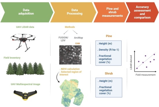
2.3. Data Acquisition by UAS

2.3.1. LiDAR Data

RPA flights (11) were conducted between 20 and 21 October 2021, covering a total area of 114.88 ha that included all of the study plots. The flights were planned to have a minimum transverse coverage of 50% between parallel passes and a minimum density of 100 points per square metre of the first return. The Unmanned Aircraft System (UAS) used was a Matrice 600 Pro equipped with a Phoenix SCOUT 16 LiDAR sensor with 16 beams and 2 returns (the strongest and the last).
The raw LiDAR data were pre-processed with Spatial Explorer 5.0 software from Phoenix LiDAR Systems, allowing extraction of valid data and colouring, georeferencing and exportation of the cloud to the desired formats. As a result, we obtained the pre-processed point cloud stored in LAS files (.las), with ellipsoidal heights, GPS time, a pass index, RGB and intensity. Finally, the point cloud was classified into ground and non-ground points using free R software [23].

2.3.2. Multispectral and RGB Data

Photogrammetric and multispectral data acquisition was carried out with an eBee RKT fixed-wing drone fitted with two cameras: RGB (true colour) and multispectral. The RGB images (Figure 3) were processed with Pix4D software and imported with the help of the creation wizard available in the same program. Data from the Global Positioning System (GPS) and the RPA position measurement unit (IMU) were combined with the RGB images and were assigned the projected coordinate system EPSG:25829 (ETRS89/UTM zone 29N).
For mapping and analysing the vegetation status, the Parrot Sequoia multispectral sensor captures a total of four bands: green, red, red edge and near infrared (NIR). The multispectral camera has a spectral sunlight sensor on top, which continuously measures and records light conditions in the same spectral bands as the multispectral sensor during the flight. The light data collected allows confirmation of the identified spectral data values. As with the true-colour images, the data were processed with Pix4D software, and radiometric calibration of the images taken in the field was conducted. Both types of images (RGB orthomosaic and multispectral) have a resolution of 8 cm/pixel.

2.4. Data Processing

The performance of two different types of software used to calculate the most important forest parameters (canopy height model, density and vegetation cover) for assessing natural regeneration were compared: Arcmap (10.2) and FUSION/LDV [24]. Both programs include a wide range of tools for processing point clouds. FUSION tools for data analysis were run by installing the add-on in QGis 3.22.0-Białowieża.
The Arcmap software (10.2) provides accurate tools that allow mapping Lidar points to produce digital terrain models (DTMs) and canopy height models (CHMs). The approach used to detect individual tree crowns was to treat the tree crown as a watershed. Both DTM and digital surface model (DSM) topographic rasters were generated using the LAS to raster data conversion function, with cell size varying between 0.5 m or 0.6 m, considering the average LAS point spacing. Using a value that is between three and four times the average point spacing is recommended to prevent the surface containing cells without data while at the same time not losing surface detail [25]. The CHM was obtained as the vertical difference between the DSM and DTM. Following the workflow shown in Figure 4, a low-pass filter was then applied to smooth and invert the CHM raster. By inverting the raster, we converted the tree canopy into watersheds and the points in the watersheds into holes. The local minima were determined using the focal flux and were finally replaced with the actual heights in the previously generated CHM.
The Fusion/LiDAR Data Viewer (LDV) software [26] was used to visualize and analyse the airborne LiDAR data. The process used to obtain the points and canopy heights consisted of 5 steps: 3 were executed by FUSION/LDV and the final 2 by SAGA, as shown in Figure 5. The “Filter Data” tool was first used to remove points with outliers, to prevent interference in future algorithms to be executed. Creation of the DTM is a key step for detecting the seedling crown points, whereby points corresponding to the ground are classified. For this purpose, the “Ground Filter” tool is run, with a resolution of 1 m x 1 m, producing the “.dtm” and “.las” files with the information corresponding to the ground.
The seedling height estimates were extracted with the “Canopy Model” algorithm, which uses the DTM together with the filtered “.las” file obtained in the first step to generate the DSM and subsequently a CHM raster. A Gaussian mean filter (Gaussian filter from SAGA) was applied to the CHM before detection of the seedling crown: this was done to increase the accuracy and correct for irregularities in the crown shape and those generated in the rasterization processes [27,28]. Finally, seedlings were located by detecting local maxima with SAGA’s “Local minimum and maximum”.
The vegetation cover was calculated using the ArcMap software with the method described by Sumerling (2011) [25]: (1) The loaded LAS file was used to define the layer by point class, i.e., by filtering of points classified as vegetation and soil individually. (2) The two-point classifications were rasterised with the “LAS point statistics as raster” tool: this step rasterises the point cloud filtered by classification to obtain the canopy cover per square unit. In the next step, (3) the No data values were replaced to 0 by applying the tools “IsNull” and “Con” for both rasters, and they were then (4) summed to obtain the total of both per cell. In the final step, (5) a division with the “Divide” tool was applied between the initial raster with the above ground density (filtered points by vegetation) with the total density, calculated in the previous step. The layer generated yields the canopy cover with values between 0 and 1, which represent the proportion of the vertical projection area of the vegetation relative to the total area [25,29].
The Fusion/LDV software speeds up extraction of vegetation cover by using the GridMetrics tool. This algorithm starts from the filtered point cloud and DTM, generating elevation and intensity statistics in CSV format. From the elevation metrics the percentage of vegetation cover (column 49) was exported to a grid in TIFF format by using the FUSION CSVaGrid tool.
Based on the available bands obtained from the multispectral sensor, the NDVI was calculated for analysis and interpretation of the different spectral regions, with the following Equation (1):
N D V I = N I R R e d N I R + R e d
The classification was based on the analysis of different spectral paths on NDVI, in order to study their behaviour and differentiate the two types of cover of interest in the study area: pine seedlings and shrubland. This was carried out with the help of the “Profile Terrain” add-on, available for free in Qgis. Different NDVI values are obtained depending on the different spectral response of the study vegetation. The variation in NDVI in one of the study plots is shown in Figure 6, in which lower values are related to sparse vegetation cover, intermediate values to scrub and higher values to pine seedlings.
The next step was to assign classes to the homogeneous pixels based on the supervised classification method with machine learning (ML) algorithms. The images were processed on the basis of the Gaussian mixture model (GMM) classifier from the Dzetsaka tools plug-in installed in Qgis software. The Dzetsaka plugin was designed to classify images directly (and quickly) from QGIS; it is a powerful add-on that supports several classification models [30,31].
The GMM model is a parametric probability density function that relies on the weighted sum of Gaussian component densities for classifying the pixels. A Gaussian mixture model is represented by the distribution shown in Equation (2):
ρ x = k = 1 k π k N x | μ k , k
where X represents the data point, K is the number of components, and µ and ∑ are the mean and covariance parameter of the multivariate Gaussian function. Each component density is a Gaussian function described as Equation (3):
ρ x | μ , = 1 2 π d / 2 1 / 2 e x p ( 1 2 ( x μ ) T 1 x μ
where πk is the weight of each Gaussian component and their sum is equal to one, 0 ≤ πk ≤ 1 [32,33].
In order to run the model, it is necessary to create training areas that are considered representative of each type of surface cover to be classified. Therefore, a vector file with regions of interest (ROI) with heterogeneous spectral signatures was created methodically, by studying the spectral variations discussed above.

2.5. Statistical Analysis

The Shapiro-Wilk test was used, being the best option to test whether the variables resulting from the structural characteristics were from a normal distribution. It was decided, in order to study the correlation between the most descriptive variables of the vegetation structure, to calculate Spearman’s non-parametric correlation coefficients (r) between the metrics derived from the field measurement (pine seedling density, pine height, shurb cover and shurb height) and those provided by LiDAR [34]. A non-parametric Wilcoxon matched pairs test was used to compare the median of the field-collected measures with the median of the LiDAR-generated calculations. Therefore, for each comparison test, the null hypothesis is that the mean difference between each pair of measurements (field measurement and LiDAR measurement) is zero (α < 0.05). [35]. All statistical analyses were performed using Rstudio software (1 July 2022 Build 554).

3. Results

3.1. Measurement Comparisons

The mean values and standard deviations for all plot parameters measured in the field and estimated by LiDAR are shown in Table 1. The field-measured mean height of the trees was 0.95 m, while the LiDAR-based estimates were 0.90 m and 0.53 m with the ArcMap and FUSION data processing methods, respectively. The pine density was around 400 ft ha−1 (although with high standard deviation values), with a field measurement of 392 ft ha−1 and LiDAR-based estimates of 403 ft ha−1 (FUSION) and 440 ft ha−1 (ArcMap). In the case of shrub height, the field-measured mean value for all plots was 0.55 m, and the LiDAR-based estimates, 0.51 m (FUSION) and 0.83 m (ArcMap).

3.2. LiDAR-Based Estimates of Vegetation Versus Field Survey Measurements

The correlation coefficients between field and LiDAR measurements obtained using ArcMap methodology, resulted different depending on the parameter considered (Figure 7). The strongest and most significant correlations were obtained for shurb cover and shrub height with r = 0.84 and r = 0.63, respectively. In the case of pine seedlings the correlations were weaker for both height (r = 0.24) and density (r = 0.16).
For the case of the LiDAR metrics with the FUSION the correlations obtained were very similar as those found with the ArcMap methodology (Figure 8).

3.3. Accuracy Assessment

The results obtained using the Wilcoxon signed-rank test (Table 2) indicate that for pine seedlings height and shrub cover the differences between field and LiDAR measurements processed with FUSION are significantly different. The remaining metrics, in both LiDAR processing methodologies, did not ststistically differ, suggesting that the estimation obtained with LiDAR can be considered satisfactory for these variables.

4. Discussion

P. pinaster seedling density measured in the present study was in the lower range of the observed post-fire seedlings density [7]. This result can be explained by the combined effect of high-severity fire (crown fire that could affect the canopy seed bank) and the lack of serotiny in the stands under study [4]. The high recovery rate of the competing shrubland is comparable to that observed in similar communities in the area [8] and may also have affected the regeneration success of P. pinaster in this area.

4.1. Visual Distribution and Differentiation of Vegetation by the NDVI

The efficiency and potential of machine learning classification algorithms, added to the high quality of multispectral images, have led to more accurate and faster land classification [36]. We used the NDVI as it is one of the most widely used, reliable and easy-to-calculate indices with the available spectral bands. In the present study, the NDVI images derived from the multispectral sensors are characterised by high spatial resolution, while satellite-based NDVIs have technical disadvantages such as the scale being too large for species and/or site-specific applications (>15–20 m), saturation phenomena and sensor-related problems [37,38]. Thus, effective use of the NDVI will depend on both the quality of the multispectral data and interpretation of the values [39,40]. The high resolution provided by the sensors during data acquisition enables more specific applications involving plant species or land cover, in contrast to NDVIs based on satellite bands, which have a much less precise resolution [37] Therefore, given the objective of this study, we required images with a low proportion of heterogeneous pixels reflecting the different types of cover at the same time [40].

4.2. Methods of LiDAR Data Processing

Previous studies comparing the same methodologies have concluded that both provide similar errors for LiDAR measurements depending on the forest conditions [41]
In the present case, and despite the difficulties due to the dense vegetation cover, the FUSION method yielded the lowest error for height estimation relative to the field measurements. This finding is consistent with that of Edson & Wing (2011), who reported that the difference between the height measured in wooded plots and LiDAR-based estimates was lower when data were processed using FUSION, with an underestimation of −0.09 m [42]. These researchers also noted that both FUSION and the ArcMap (watershed method) correctly determined large trees, but that the latter performed better for detecting smaller trees. The absence of any great difference in the results obtained with the watershed method and the FUSION method in the present study can therefore be attributed to the lack of large differences in height between pine seedlings and shrubs.
Tree crowns are usually extracted from the CHM as local maxima. However, this can lead to errors in complex forest structures, as multiple local maxima can be identified in the same irregularly shaped canopy and errors can also occur in creating the CHM [43,44]. For canopy detection, we therefore applied a Gaussian filter to the output created by FUSION and to invert the CHM and subsequent apply a low filter in the watershed method, thus making canopy detection more intuitive. Filters should be applied to high density point clouds, as there will be a higher number of hits in the same canopy [45].
In short, comparison of the precision of the estimation of the studied parameters is complicated by the lack of previous research involving dense, mixed vegetation compositions with different strata.

4.3. Influence of Vegetation Structure on LiDAR-Based Estimates

Correlations between measured and estimated LiDAR parameters at plot level for pine seedlings variables (r height ≤ 0.24, r density ≤ 0.33) were not as high as for shrubland (r height 0.50–0.63, r cover = 0.84), which was attributed to the fact that LiDAR was unable to measure the lower canopy layers (pine seedlings) with good accuracy, as opposed to the upper layers (shrubland) [46]. Therefore, interference from occlusion could be a problem in the detection of small pine trees that ultimately manifests itself in low correlations for their metrics. The effects and mitigation of occlusion in laser scanning is still being studied today for different vegetation conformations [47,48].
In this context, where the effects of vegetation structure and the response of LiDAR pulses influence the measured parameters, such as vegetation cover. Research focused on estimating vegetation cover shows that the information loss coefficient is much higher in forested areas than in open terrain [49]. Other factors affected by the depth of vegetation, resulting in loss of points and information, include the distribution of the backscatter cross-section, the trajectory of laser pulses and the degree of energy attenuation [49,50].
The loss of canopy information due to the complexity of the vegetation in the present study may have been minimised by the availability of high point density data [51,52]. Finally, taking into account the complex terrain and vegetation structure in the study area, the parameter estimates obtained are encouraging and support the use of LiDAR technologies in areas where they have not previously been applied.
Another interesting point for discussion would be the plot size used. However, the error in the measured parameters is not particularly attributable to the chosen plot size as an approximate plot size of 25 m diameter is standard in temperate forest inventories [53,54,55]. In addition, stand variability will determine the number of plots needed [56]. In relation to this aspect, studies such as those by Hernández-Stefanoni et al. (2018) have already assessed the impacts of plot size on the precision of aerial biomass estimates predicted from LiDAR data, in which they determined that the precision of LiDAR estimates will be proportionally higher with sample plot size. In the same paper, they also studied how plot size would affect GPS location errors, which also increased with increasing plot size. They attributed this to a higher degree of spatial overlap between the sample plot and the LiDAR data on larger plots [57]. However, although the size of the plots (40 m x 40 m) reflect the variability in terms of regeneration in a specific area burned with a certain degree of fire severity, the number of plots used in the study also may affected the obtained results.

5. Conclusions

The use and integration of multispectral images together with LiDAR data may have great potential for use in post-fire forests, where an assessment of the condition of the forest stands is required in view of the need for reforestation due to poor regeneration.
In this study, different methods of extracting the most important parameters characterizing forest cover were tested in a context of complex vegetation structure and composition. In addition, two methods of processing LiDAR data were compared in order to determine which provided the most accurate estimates, relative to field-measured data.
From the overall mean values of tree height obtained for all plots, the ArcMap data processing method produced values that were similar to the field data. However, for shrub height, the FUSION method was more accurate, as ArcMap tended to slightly overestimate the values. Linear regression revealed a weak relationship between the estimated tree heights and the field measured values. The poor correlation was attributed to the naturally occurring vegetation consisting of tall, dense scrub, which can cause larger errors in LiDAR-based height estimation.
The high density of points was very useful for preventing major errors due to the limitations of laser penetration in the dense scrub, providing a better outcome. However, this did not prevent the occlusion effect produced by the higher heights of the scrub, together with the low representativeness of the pine in some of the plots, from producing a lower accuracy in the measurements of pine regeneration.
In conclusion, this study aims to highlight the need to introduce LiDAR in more complex and less usual applications, where the conformation of the vegetation raises the difficulty of obtaining better accuracies, revealing necessary points to improve/study. It also includes methodologies for post-flight data processing and management.
Therefore, further studies should be conducted in areas characterized by dense scrub cover and low vegetation, which imply greater difficulty both for the LiDAR measurement and the subsequent data processing. This would help to improve the accuracy of LiDAR-based estimates relative to conventional field methods depending on the conditions in the study area.

Author Contributions

Conceptualization, C.M. and C.F.; methodology, C.M. and C.F.; software, C.M.; validation, C.M. and C.F.; formal analysis, C.M. and C.F.; investigation, C.M. and C.F.; data curation, C.M. and C.F.; writing—original draft preparation, C.M. and C.F.; visualization, C.M. and C.F.; supervision, C.F.; project administration, C.F.; funding acquisition, C.F. All authors have read and agreed to the published version of the manuscript.

Funding

This research was funded by the Spanish Research Agency of the Spanish Ministry of Science and Innovation through project ENFIRES-NW, PID2020-116494RR-C42.

Data Availability Statement

The datasets used or analysed during the study will be made available upon reasonable request.

Acknowledgments

Authors acknowledge CETEMAS foundation for the technical assistance with the UAVS flights and José Gómez, Jesús Pardo and Emilia Puga for their help with the field work.

Conflicts of Interest

The authors declare no conflict of interest. The funders had no role in the design of the study; in the collection, analysis or interpretation of data; in the writing of the manuscript; or in the decision to publish the results.

References

  1. Vega, J.A.; Pérez, S.A.; Fernández, C.; Lliteras, M.T.F.; González, A.D.R. Os incendios forestais do cambio global xa están aquí: Un desafío e unha ocasión para lograr unha resposta social consensuada. In Unha Nova Xeración de Lumes?: Actas do Coloquio Galaico-Portugués Sobre Incendios Forestais; Consello da Cultura Galega: Santiago de Compostela, Spain, 2021. [Google Scholar] [CrossRef]
  2. European Commission, Joint Research Centre; Camia, A.; Libertá, G.; San-Miguel-Ayanz, J. Modeling the Impacts of Climate Change on Forest Fire Danger in Europe: Sectorial results of the PESETA II Project; Publications Office: Luxembourg, 2017. [Google Scholar] [CrossRef]
  3. Fernandes, P.M.; Rigolot, E. The fire ecology and management of maritime pine (Pinus pinaster Ait.). For. Ecol. Manag. 2007, 241, 1–13. [Google Scholar] [CrossRef]
  4. Fernández, C.; Vega, J.A.; Fonturbel, T.; Jiménez, E.; Pérez-Gorostiaga, P. Effects of wildfire, salvage logging and slash manipulation on Pinus pinaster Ait. recruitment in Orense (NW Spain). For. Ecol. Manag. 2008, 255, 1294–1304. [Google Scholar] [CrossRef]
  5. Vega, J.A.; Fernández, C.; Pérez-Gorostiaga, P.; Fonturbel, T. Response of maritime pine (Pinus pinaster Ait.) recruitment to fire severity and post-fire management in a coastal burned area in Galicia (NW Spain). Plant Ecol. 2010, 206, 297–308. [Google Scholar] [CrossRef]
  6. Calvo, L.; Santalla, S.; Valbuena, L.; Marcos, E.; Tárrega, R.; Luis-Calabuig, E. Post-fire natural regeneration of a Pinus pinaster forest in NW Spain. Plant Ecol. 2008, 197, 81–90. [Google Scholar] [CrossRef]
  7. Lucas-Borja, M.; Plaza-Álvarez, P.; González-Romero, J.; Miralles, I.; Sagra, J.; Molina-Peña, E.; Moya, D.; Heras, J.D.L.; Fernández, C. Post-wildfire straw mulching and salvage logging affects initial pine seedling density and growth in two Mediterranean contrasting climatic areas in Spain. For. Ecol. Manag. 2020, 474, 118363. [Google Scholar] [CrossRef]
  8. Fernández, C.; Vega, J.A.; Fonturbel, T. Does shrub recovery differ after prescribed burning, clearing and mastication in a Spanish heathland? Plant Ecol. 2015, 216, 429–437. [Google Scholar] [CrossRef]
  9. Yang, J.; Pan, S.; Dangal, S.; Zhang, B.; Wang, S.; Tian, H. Continental-scale quantification of post-fire vegetation greenness recovery in temperate and boreal North America. Remote Sens. Environ. 2017, 199, 277–290. [Google Scholar] [CrossRef]
  10. Gouveia, C.; DaCamara, C.C.; Trigo, R.M. Post-fire vegetation recovery in Portugal based on spot/vegetation data. Nat. Hazards Earth Syst. Sci. 2010, 10, 673–684. [Google Scholar] [CrossRef] [Green Version]
  11. Meng, R.; Dennison, P.E.; Huang, C.; Moritz, M.A.; D’Antonio, C. Effects of fire severity and post-fire climate on short-term vegetation recovery of mixed-conifer and red fir forests in the Sierra Nevada Mountains of California. Remote Sens. Environ. 2015, 171, 311–325. [Google Scholar] [CrossRef]
  12. Veraverbeke, S.; Hook, S.; Hulley, G. An alternative spectral index for rapid fire severity assessments. Remote Sens. Environ. 2012, 123, 72–80. [Google Scholar] [CrossRef]
  13. Lu, D.; Chen, Q.; Wang, G.; Liu, L.; Li, G.; Moran, E. A survey of remote sensing-based aboveground biomass estimation methods in forest ecosystems. Int. J. Digit. Earth 2016, 9, 63–105. [Google Scholar] [CrossRef]
  14. Wulder, M.; White, J.; Alvarez, F.; Han, T.; Rogan, J.; Hawkes, B. Characterizing boreal forest wildfire with multi-temporal Landsat and LIDAR data. Remote Sens. Environ. 2009, 113, 1540–1555. [Google Scholar] [CrossRef]
  15. Martín-Alcón, S.; Coll, L.; De Cáceres, M.; Guitart, L.; Cabré, M.; Just, A.; González-Olabarría, J.R. Combining aerial LiDAR and multispectral imagery to assess postfire regeneration types in a Mediterranean forest. Can. J. For. Res. 2015, 45, 856–866. [Google Scholar] [CrossRef]
  16. Zhao, J.; Zhao, L.; Chen, E.; Li, Z.; Xu, K.; Ding, X. An Improved Generalized Hierarchical Estimation Framework with Geostatistics for Mapping Forest Parameters and Its Uncertainty: A Case Study of Forest Canopy Height. Remote Sens. 2022, 14, 568. [Google Scholar] [CrossRef]
  17. Rahman, F.; Onoda, Y.; Kitajima, K. Forest canopy height variation in relation to topography and forest types in central Japan with LiDAR. For. Ecol. Manag. 2022, 503, 119792. [Google Scholar] [CrossRef]
  18. Gatziolis, D.; Fried, J.S.; Monleon, V.S. Challenges to Estimating Tree Height via LiDAR in Closed-Canopy Forests: A Parable from Western Oregon. For. Sci. 2010, 56, 139–155. [Google Scholar]
  19. Novo-Fernández, A.; Barrio-Anta, M.; Recondo, C.; Cámara-Obregón, A.; López-Sánchez, C.A. Integration of National Forest Inventory and Nationwide Airborne Laser Scanning Data to Improve Forest Yield Predictions in North-Western Spain. Remote Sens. 2019, 11, 1693. [Google Scholar] [CrossRef] [Green Version]
  20. Kellner, J.R.; Armston, J.; Birrer, M.; Cushman, K.C.; Duncanson, L.; Eck, C.; Falleger, C.; Imbach, B.; Král, K.; Krůček, M.; et al. New Opportunities for Forest Remote Sensing through Ultra-High-Density Drone Lidar. Surv. Geophys. 2019, 40, 959–977. [Google Scholar] [CrossRef] [Green Version]
  21. World Soil Resources Reports. World Reference Base for Soil Resources 2014, Update 2015: International Soil Classification System for Naming Soils and Creating Legends for Soil Maps; FAO: Rome, Italy, 2015. [Google Scholar]
  22. Canfield, R.H. Application of the line interception method in sampling range vegetation. J. For. 1941, 39, 388–394. [Google Scholar] [CrossRef]
  23. Roussel, J.-R.; Auty, D.; Coops, N.C.; Tompalski, P.; Goodbody, T.R.; Meador, A.S.; Bourdon, J.-F.; de Boissieu, F.; Achim, A. lidR: An R package for analysis of Airborne Laser Scanning (ALS) data. Remote Sens. Environ. 2020, 251, 112061. [Google Scholar] [CrossRef]
  24. McGaughey, B. FUSION/LDV LIDAR Analysis and Visualization Software. Available online: http://forsys.cfr.washington.edu/fusion/fusion_overview.html (accessed on 12 December 2022).
  25. Sumerling, G. Lidar Analysis in ArcGIS® 10 for Forestry Applications; Esri: Redlands, CA, USA, 2011. [Google Scholar]
  26. USDA. Pacific Northwest Research Station. Available online: https://www.fs.usda.gov/pnw/ (accessed on 28 November 2022).
  27. Harikumar, A.; Bovolo, F.; Bruzzone, L. A Local Projection-Based Approach to Individual Tree Detection and 3-D Crown Delineation in Multistoried Coniferous Forests Using High-Density Airborne LiDAR Data. IEEE Trans. Geosci. Remote Sens. 2018, 57, 1168–1182. [Google Scholar] [CrossRef]
  28. Barnes, C.; Balzter, H.; Barrett, K.; Eddy, J.; Milner, S.; Suárez, J.C. Individual Tree Crown Delineation from Airborne Laser Scanning for Diseased Larch Forest Stands. Remote Sens. 2017, 9, 231. [Google Scholar] [CrossRef] [Green Version]
  29. Zhang, S.; Chen, H.; Fu, Y.; Niu, H.; Yang, Y.; Zhang, B. Fractional Vegetation Cover Estimation of Different Vegetation Types in the Qaidam Basin. Sustainability 2019, 11, 864. [Google Scholar] [CrossRef] [Green Version]
  30. Karasiak, N.; Perbet, P. Remote Sensing of Distinctive Vegetation in Guiana Amazonian Park. In QGIS and Applications in Agriculture and Forest; John Wiley & Sons, Ltd.: London, UK, 2018; pp. 215–245. [Google Scholar] [CrossRef]
  31. Santarsiero, V.; Nolè, G.; Lanorte, A.; Tucci, B.; Cillis, G.; Murgante, B. Remote Sensing and Spatial Analysis for Land-Take Assessment in Basilicata Region (Southern Italy). Remote Sens. 2022, 14, 1692. [Google Scholar] [CrossRef]
  32. Reynolds, D. Gaussian Mixture Models. In Encyclopedia of Biometrics; Li, S.Z., Jain, A., Eds.; Springer: Boston, MA, USA, 2009; pp. 659–663. [Google Scholar] [CrossRef]
  33. Xing, Y.; Lv, C.; Cao, D. Chapter 4—Design of Integrated Road Perception and Lane Detection System for Driver Intention Inference. In Advanced Driver Intention Inference; Xing, Y., Lv, C., Cao, D., Eds.; Elsevier: Amsterdam, The Netherlands; Oxford, UK; Cambridge, MA, USA, 2020; pp. 77–98. [Google Scholar] [CrossRef]
  34. Ochoa-Franco, A.D.P.; Valdez-Lazalde, J.R.; Ángeles-Pérez, G.; Santos-Posadas, H.M.D.L.; Hernández-Stefanoni, J.L.; Valdez-Hernández, J.I.; Pérez-Rodríguez, P. Beta-Diversity Modeling and Mapping with LiDAR and Multispectral Sensors in a Semi-Evergreen Tropical Forest. Forests 2019, 10, 419. [Google Scholar] [CrossRef] [Green Version]
  35. Hummel, S.; Hudak, A.T.; Uebler, E.H.; Falkowski, M.J.; Megown, K.A. A Comparison of Accuracy and Cost of LiDAR versus Stand Exam Data for Landscape Management on the Malheur National Forest. J. For. 2011, 109, 267–273. [Google Scholar]
  36. Mahboubi, M.; Belcore, E.; Pontoglio, E.; Matrone, F.; Lingua, A. Detection of Wet Riparian Areas using Very High Resolution Multispectral UAS Imagery Based on a Feature-based Machine Learning Algorithm. AGILE GISci. Ser. 2022, 3, 46. [Google Scholar] [CrossRef]
  37. Gómez-Sapiens, M.; Schlatter, K.J.; Meléndez, Á.; Hernández-López, D.; Salazar, H.; Kendy, E.; Flessa, K.W. Improving the efficiency and accuracy of evaluating aridland riparian habitat restoration using unmanned aerial vehicles. Remote Sens. Ecol. Conserv. 2021, 7, 488–503. [Google Scholar] [CrossRef]
  38. Prăvălie, R.; Sîrodoev, I.; Nita, I.-A.; Patriche, C.; Dumitraşcu, M.; Roşca, B.; Tişcovschi, A.; Bandoc, G.; Săvulescu, I.; Mănoiu, V.; et al. NDVI-based ecological dynamics of forest vegetation and its relationship to climate change in Romania during 1987–2018. Ecol. Indic. 2022, 136, 108629. [Google Scholar] [CrossRef]
  39. Huang, S.; Tang, L.; Hupy, J.P.; Wang, Y.; Shao, G. A commentary review on the use of normalized difference vegetation index (NDVI) in the era of popular remote sensing. J. For. Res. 2021, 32, 1–6. [Google Scholar] [CrossRef]
  40. Lima-Cueto, F.J.; Blanco-Sepúlveda, R.; Gómez-Moreno, M.L.; Galacho-Jiménez, F.B. Using Vegetation Indices and a UAV Imaging Platform to Quantify the Density of Vegetation Ground Cover in Olive Groves (Olea Europaea L.) in Southern Spain. Remote Sens. 2019, 11, 2564. [Google Scholar] [CrossRef] [Green Version]
  41. Mcgaughey, R.J.; Reutebuch, S.E. Forest Measurement and Monitoring Using High-Resolution Airborne Lidar Biophysical Controls on Forest Structure and Fire Severity in Yosemite National Park View Project. 2005. Available online: https://www.researchgate.net/publication/237253220 (accessed on 1 November 2022).
  42. Edson, C.; Wing, M.G. Airborne Light Detection and Ranging (LiDAR) for Individual Tree Stem Location, Height, and Biomass Measurements. Remote Sens. 2011, 3, 2494–2528. [Google Scholar] [CrossRef] [Green Version]
  43. Mu, Y.; Fujii, Y.; Takata, D.; Zheng, B.; Noshita, K.; Honda, K.; Ninomiya, S.; Guo, W. Characterization of peach tree crown by using high-resolution images from an unmanned aerial vehicle. Hortic. Res. 2018, 5, 74. [Google Scholar] [CrossRef] [PubMed] [Green Version]
  44. Panagiotidis, D.; Abdollahnejad, A.; Surový, P.; Chiteculo, V. Determining tree height and crown diameter from high-resolution UAV imagery. Int. J. Remote Sens. 2017, 38, 2392–2410. [Google Scholar] [CrossRef]
  45. Kumar, V. Forest Inventory Parameters and Carbon Mapping from Airborne LIDAR. 2012. Available online: http://essay.utwente.nl/84846/ (accessed on 5 November 2022).
  46. Venier, L.A.; Swystun, T.; Mazerolle, M.J.; Kreutzweiser, D.P.; Wainio-Keizer, K.L.; McIlwrick, K.A.; Woods, M.E.; Wang, X. Modelling vegetation understory cover using LiDAR metrics. PLoS ONE 2019, 14, e0220096. [Google Scholar] [CrossRef] [Green Version]
  47. Schneider, F.D.; Kükenbrink, D.; Schaepman, M.E.; Schimel, D.S.; Morsdorf, F. Quantifying 3D structure and occlusion in dense tropical and temperate forests using close-range LiDAR. Agric. For. Meteorol. 2019, 268, 249–257. [Google Scholar] [CrossRef]
  48. Mathes, T.; Seidel, D.; Häberle, K.-H.; Pretzsch, H.; Annighöfer, P. What Are We Missing? Occlusion in Laser Scanning Point Clouds and Its Impact on the Detection of Single-Tree Morphologies and Stand Structural Variables. Remote Sens. 2023, 15, 450. [Google Scholar] [CrossRef]
  49. Liu, Q.; Fu, L.; Wang, G.; Li, S.; Li, Z.; Chen, E.; Pang, Y.; Hu, K. Improving Estimation of Forest Canopy Cover by Introducing Loss Ratio of Laser Pulses Using Airborne LiDAR. IEEE Trans. Geosci. Remote Sens. 2019, 58, 567–585. [Google Scholar] [CrossRef]
  50. Garroway, K.; Hopkinson, C.; Jamieson, R. Surface moisture and vegetation influences on lidar intensity data in an agricultural watershed. Can. J. Remote Sens. 2011, 37, 275–284. [Google Scholar] [CrossRef]
  51. Kandare, K.; Ørka, H.O.; Chan, J.C.-W.; Dalponte, M. Effects of forest structure and airborne laser scanning point cloud density on 3D delineation of individual tree crowns. Eur. J. Remote Sens. 2016, 49, 337–359. [Google Scholar] [CrossRef] [Green Version]
  52. Magnusson, M.; Fransson, J.E.; Holmgren, J. Effects on estimation accuracy of forest variables using different pulse density of laser data. For. Sci. 2007, 53, 619–626. [Google Scholar] [CrossRef]
  53. Hamrouni, A.; Véga, C.; Renaud, J.P.; Durrieu, S.; Bouvier, M. A tree-based approach to estimate wood volume from lidar data: A case study in a pine plantation. Rev. Française Photogramm. Télédétect. 2015, 1, 63–70. [Google Scholar] [CrossRef]
  54. Castaño-Díaz, M.; Álvarez-Álvarez, P.; Tobin, B.; Nieuwenhuis, M.; Afif-Khouri, E.; Cámara-Obregón, A. Evaluation of the use of low-density LiDAR data to estimate structural attributes and biomass yield in a short-rotation willow coppice: An example in a field trial. Ann. For. Sci. 2017, 74, 69. [Google Scholar] [CrossRef] [Green Version]
  55. Levick, S.R.; Hessenmöller, D.; Schulze, E.-D. Scaling wood volume estimates from inventory plots to landscapes with airborne LiDAR in temperate deciduous forest. Carbon Balance Manag. 2016, 11, 7. [Google Scholar] [CrossRef] [Green Version]
  56. US Department of Agriculture, Resources Conservation Service. Title 190-Forestry Inventory Methods Technical Note Forestry Inventory Methods. 2018. Available online: www.ascr.usda.gov (accessed on 10 November 2022).
  57. Hernández-Stefanoni, J.L.; Reyes-Palomeque, G.; Castillo-Santiago, M.; George-Chacón, S.P.; Huechacona-Ruiz, A.H.; Tun-Dzul, F.; Rondon-Rivera, D.; Dupuy, J.M. Effects of Sample Plot Size and GPS Location Errors on Aboveground Biomass Estimates from LiDAR in Tropical Dry Forests. Remote Sens. 2018, 10, 1586. [Google Scholar] [CrossRef] [Green Version]
Figure 1. Location of the study site.
Remotesensing 15 01634 g001
Figure 2. Partial view of the study site.
Remotesensing 15 01634 g002
Figure 3. Orthomosaic RGB image.
Remotesensing 15 01634 g003
Figure 4. Workflow in ArcMap.
Remotesensing 15 01634 g004
Figure 5. FUSION/LDV workflow.
Remotesensing 15 01634 g005
Figure 6. Variations in the spectral signature.
Remotesensing 15 01634 g006
Figure 7. Spearman’s correlation coefficients (AD) between variables measured in the field and those estimated by LiDAR + ArcMap.
Remotesensing 15 01634 g007
Figure 8. Spearman’s correlation coefficients (AD) between variables measured in the field and those estimated by LiDAR + FUSION.
Remotesensing 15 01634 g008
Table 1. Mean values and standard deviation (SD) of pine and shrub characteristics.
Field MeasurementLiDAR-Based Estimate
Fusion
ArcMap
MeanSDMeanSDMeanSD
Pine
Height (m)0.950.200.530.140.900.24
Density (ft ha−1)392.25267.80403.71145.25440.63161.20
Shrub
Height (m)0.550.290.510.350.830.41
Cover (%)79.4219.9223.057.2881.136.09
Table 2. Wilcoxon Signed Rank Test Results. Differences resulted significant when p-value < 0.05.
p-Value
LiDAR Processing MethodArcMapFusion
Pine
Height (m)0.2990.023
Density (ft ha−1)0.6640.895
Shrub
Height (m)0.0550.650
Cover (%)0.5090.003
Disclaimer/Publisher’s Note: The statements, opinions and data contained in all publications are solely those of the individual author(s) and contributor(s) and not of MDPI and/or the editor(s). MDPI and/or the editor(s) disclaim responsibility for any injury to people or property resulting from any ideas, methods, instructions or products referred to in the content.

