Article

Improved the Characterization of Flood Monitoring Based on Reconstructed Daily GRACE Solutions over the Haihe River Basin

1
School of Geomatics, Liaoning Technical University, Fuxin 123000, China
2
School of Surveying and Landing Information Engineering, Henan Polytechnic University, Jiaozuo 454000, China
3
China Academy of Aerospace Science and Innovation, China Aerospace Science and Technology Corporation, Beijing 100176, China
4
Ministry of Ecology and Environment Center for Satellite Application on Ecology and Environment, Beijing 100089, China
5
School of Geography and Information Engineering, China University of Geosciences, Wuhan 430078, China
*
Author to whom correspondence should be addressed.
These authors contributed equally to this paper.
Remote Sens. 2023, 15(6), 1564; https://doi.org/10.3390/rs15061564
Submission received: 7 February 2023 / Revised: 4 March 2023 / Accepted: 9 March 2023 / Published: 13 March 2023

Abstract

:
Flood events have caused huge disasters with regard to human life and economic development, especially short-term flood events that have occurred in recent years. Gravity Recovery and Climate Experiment (GRACE) satellites can directly detect the spatiotemporal characteristics of terrestrial water storage anomalies (TWSA), which play an important role in capturing flood signals. However, the monthly resolution of GRACE-derived TWSA limits its application in monitoring sub-monthly flood events. Therefore, this paper first reconstructs the daily TWSA based on a statistical model with near real-time precipitation and temperature as input variables, and then three daily flood monitoring indexes are developed based on the reconstructed TWSA. Furthermore, these indexes are employed to evaluate the temporal and spatial characteristics of the 2016 short-term flood event in the Haihe River basin (HRB), including the flood potential index (FPI), water storage deficit index (WSDI), and combined climate deviation index (CCDI). In contrast to previous studies, the temporal resolution of TWSA-based indexes is improved from the monthly scale to the daily scale, which largely improves the temporal characterization of flood monitoring. Results demonstrate that (1) among ten kinds of “Temperature-Precipitation” combinations, the reconstructed TWSA based on CN05.1-CN05.1 match well with the GRACE TWSA, as well as publicly available daily TWSA datasets with a Nash-Sutcliffe efficiency coefficient (NSE) of 0.96 and 0.52 ~ 0.81 respectively. (2) The short-term flood characteristics can be better characterized by the reconstructed daily TWSA based on CN05.1-CN05.1, reaching the peak of 216.19 mm on July 20 in the flood center. Additionally, the spatial characteristics of the equivalent water height (EWH) are detected to evolve from southwest to northeast during the short-term flood. (3) FPI, WSDI, and CCDI are proven to be effective in monitoring flood events in the HRB, which validates the reliability of the reconstructed daily TWSA. Moreover, compared to the 56% and 66% coverage of damage quantified by FPI and CCDI, the 45% damage coverage of the flood mapped by WSDI is more consistent with the governmental reports within the HRB. This paper is expected to provide a valuable reference for the assessment of short-term events caused by extreme climate change.

1. Introduction

Global warming has accelerated the water cycle, leading to an increase in the frequency and severity of droughts and floods, which seriously hinder the development of human society and the economy [1,2]. Normally, flooding is difficult to evaluate accurately [3], and flood monitoring is facing serious challenges under the conditions of extreme climate change. As one of the flood-prone countries, many areas have suffered from flood damage in China, such as the Yangtze River basin (YRB) and the Pearl River basin (PRB) [4,5,6]. According to the Ministry of Water Resources of the People’s Republic of China (MWR), the economic losses directly caused by floods exceeded 410 billion dollars from 2010 to 2020, and the total number of people affected reached 1 billion [7]. Floods have become a major meteorological disaster affecting the economic development of China. Therefore, there is an urgent need to monitor flood events in a timely and accurate manner, which can help to reduce economic losses and contribute to sustainable development.
Nevertheless, it is challenging to monitor floods based on traditional methods. In situ stations can provide accurate information about the precipitation and streamflow, however, uneven spatial distribution makes it difficult to cope with widespread damage [8]. Some models based on geographic features and hydrological information can detect floods with high spatial resolution in a timely manner, but they require collaboration among different software and the support of abundant data [9,10]. In addition, remote sensing technology provides a new tool for wide-scale flood monitoring, which can accurately portray the spatial evolution of floods [11,12]. However, this approach is expensive and cannot detect the water variation of all components in terrestrial areas since it neglects the response of soil moisture, which is often regarded as a substitute data for flood monitoring according to some available studies [13,14,15].
Gravity Recovery and Climate Experiment (GRACE) satellite mission and its successor GRACE Follow-On (GRACE-FO) can monitor the terrestrial water storage anomalies (TWSA) by detecting the changes in Earth’s gravity field [16,17,18]. More importantly, the TWSA plays an important role in capturing flood signals [19], because it comprises all the forms of water stored under and above the earth [20,21]. Thus, some TWSA-based indexes have contributed significantly to large-scale flood monitoring. Specifically, the flood potential index (FPI) was first proposed based on TWSA by Reager and Famiglietti [22]. They verified its applicability on a global scale by comparing it with the data of hydrology stations. Subsequently, flood events in different areas were evaluated by FPI and made good progress. For example, Sun et al. [4] used FPI to explore the 2010 flood event in the YRB, and demonstrated that FPI can reliably assess extreme hydrological variability with high temporal and spatial resolution. Idowu and Zhou [23] estimated the 2012 flood event in Nigeria based on FPI, and the results were generally consistent with the records of hydrological observatories. In addition, min-max normalization and the probability density function were used to construct an improved FPI, which achieved reasonable effectiveness in the PRB [24] and Southwest China [25]. In recent years, GRACE-derived indexes based on standardized ideas have been used to evaluate extreme climate change. For instance, the combined climate deviation index (CCDI) was developed by Sinha et al. to explore extreme climate events in the major river basins within India, which suggested that CCDI is more efficient in areas with abundant rainfall [26]. Nigatu et al. [27] assessed eight major flood events in the Nile basin using the water storage deficits index (WSDI), and the results indicated that WSDI matches well with reality compared with the palmer drought severity index (PDSI). Additionally, some drought indexes have been developed, such as the Discrepancy Precipitation Index (DPI) [28] and total storage deficit index (TSDI) [29], which effectively contribute to the assessment of drought events in different regions. Unfortunately, the above indexes are limited by the rough temporal resolution of GRACE TWSA, which makes it difficult to capture the finer characteristics of the short-term meteorological events, such as the “Zhengzhou 7.20” flood in 2021 [30]. Therefore, the daily scale TWSA is urgently needed to improve the temporal characterization of flood monitoring.
To obtain the daily TWSA, a Kalman filter approach based on GRACE data was utilized to obtain the daily solutions [31], which confirmed that it is helpful in assessing flood events over the Ganges-Brahmaputra Delta in 2004 and 2007 [32]. Moreover, Xiong et al. [33] developed a daily standardized drought and flood potential index (SDFPI) based on the random forest (RF) model and ITSG-Grace2018, which successfully evaluated the short-term flood and drought events from 1961 to 2015 in the YRB. However, as the current publicly released daily gravity field solution, ITSG-Grace2018 is not capable of meeting the near real-time monitoring for flood events, because the latency in the releasing of data takes several months [30]. Additionally, Jiang et al. [34] combined the Global Navigation Satellite System (GNSS) and GRACE data to evaluate the change of TWSA in Yunnan, suggesting that GNSS networks can track TWSA with a daily resolution during extreme weather events, however, there are difficulties in acquiring GNSS data. Recently, Humphrey and Gudmundsson [35] established a statistical model according to the hydrological modeling principle, which effectively reconstructed the monthly and daily TWSA (such as the JPL-ERA5) with the spatial resolution of 0.5° × 0.5°. This model is constrained by GRACE TWSA and widely applied because of its effectiveness and low cost [36,37,38].
In this study, a statistical model taking real-time precipitation and temperature as input variables is used to reconstruct the daily TWSA over the Haihe River basin (HRB), and reconstructed TWSA are further applied to construct daily monitoring indexes to assess the short-term flood event that occurred in 2016. The primary objectives of this work are as follows: (1) to collect meteorological data from different sources and compare reconstructed TWSA in the HRB based on that information, (2) to evaluate the change in water volume of the reconstructed daily TWSA, and (3) to evaluate and analyze the effectiveness of daily flood monitoring indexes in a short-term flood event from the perspectives time evolution and spatial distribution.

2. Materials and Methods
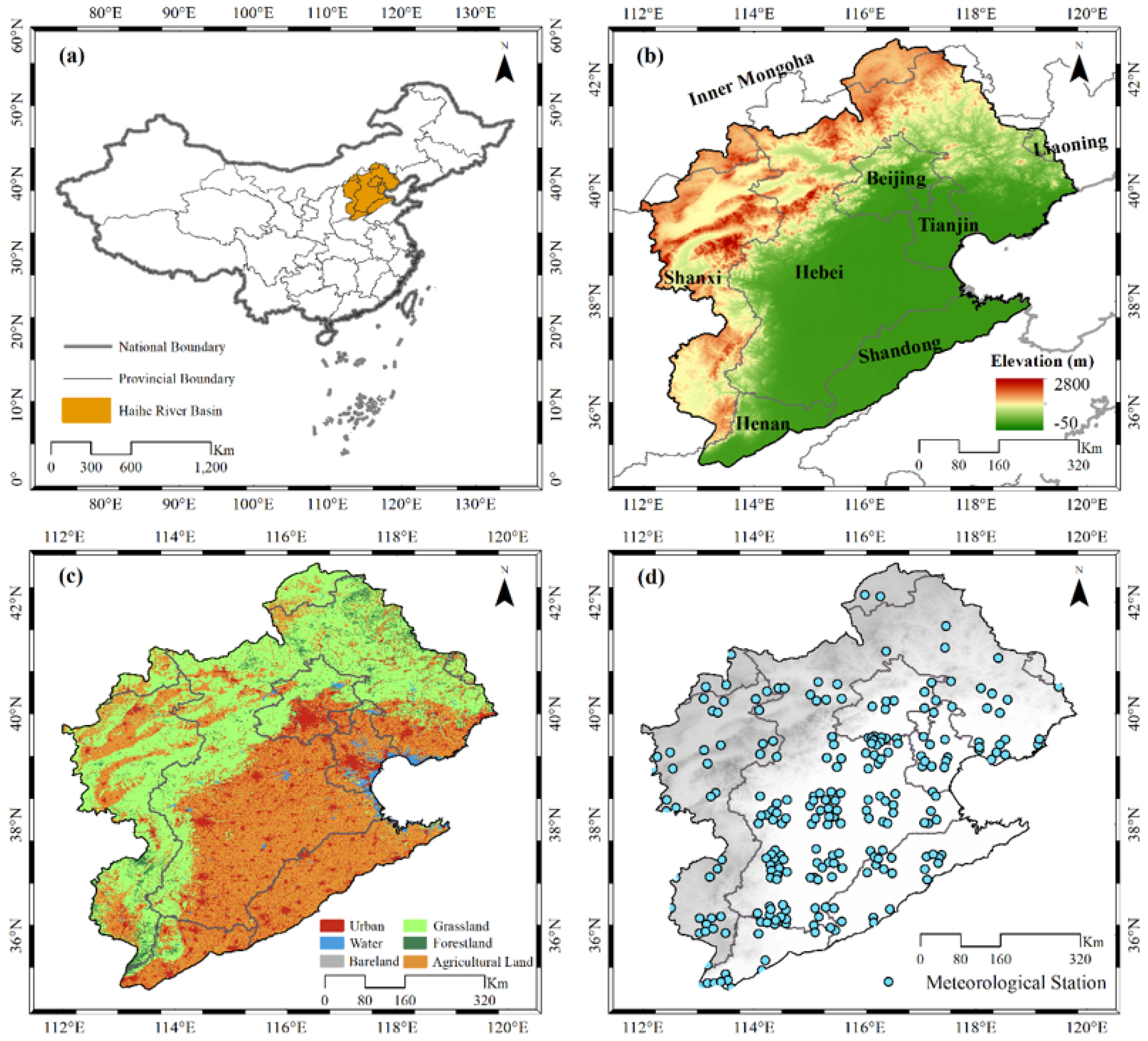
2.1. Study Area

The Haihe River basin (HRB) is located in North China, between 112°~120°E and 35°~43°N, with an area of approximately 3.2 × 10⁵ km² (Figure 1a). Its total topography is high in the northwest and low in the southeast. The HRB spans eight provinces or cities (Figure 1b), and the plains area in the southeast is a concentrated area of agriculture and cities (Figure 1c). There are 234 meteorological stations within the HRB, mainly concentrated in the North China Plain (Figure 1d). Precipitation mostly occurs in the flood season (June ~ October), and there is often a high probability of flooding due to extreme rainfall during this period [39]. Nevertheless, precipitation is less from March to May when crop water demand reaches its peak. Due to agricultural irrigation, the water resources are in a deficit state [40,41]. The decrease in water quantity has received great attention, especially under the influence of human activities [42,43]. However, little research has been done on the flooding that occurs in this basin. It has been recorded that the HRB experienced severe flooding in July 2012 [44], July 2016 (http://www.gov.cn/xinwen/2016-07/21/content_5093878.htm, accessed on 1 July 2022), and July–October 2021 (http://www.hwcc.gov.cn/sxdzt/mt2021hwccfxgz/202110/t20211022_97487.html, accessed on 2 July 2022).

2.2. Data

2.2.1. GRACE/GRACE-FO Solutions

The changes of TWS can be derived by GRACE satellites with an unprecedented accuracy, and its products are classified into spherical harmonic and mascon solutions [45,46]. Compared to spherical harmonic products, mascon solutions are able to reduce signal leakage in the sea–land interface and do not require filter methods to eliminate north-south strip errors [47]. Monthly release-06 (RL06) solutions are utilized in this study, which are provided by the Center for Space Research (CSR, https://www2.csr.utexas.edu/grace/, accessed on 1 June 2022) and the Jet Propulsion Laboratory (JPL, https://grace.jpl.nasa.gov/, accessed on 1 June 2022). To reduce leakage bias, scale factor solutions are used to enrich the JPL RL06 data, which are provided by the global Community Land Model (CLM4.0) [48,49].
The TWSA accounts for the anomaly of the equivalent water height (EWH) relative to the mean baseline from 2004 to 2009. To ensure the accuracy of data, CSR and JPL solutions are averaged to estimate the TWSA with a spatial resolution of 0.25° × 0.25°. It should be noted that there is an 11-month data gap between GRACE and GRACE-FO. Many approaches have been applied to fill this gap and have achieved reasonable performance, including Long-term Precipitation Driven (LPD) [43,50], Bayesian Convolutional Neural Network (BCNN) [51], and a Bayesian Framework (BF) [52]. Moreover, the missing data due to battery management are estimated through linear interpolation [53], information of the reconstructed TWSA products is shown in Table 1.

2.2.2. Meteorological Data

Daily precipitation and temperature are important driving variables for the reconstruction of TWSA [35]. Considering the spatiotemporal characteristics of remote sensing products, five kinds of precipitation and two temperature datasets are collected and classified into ten “Temperature-Precipitation” combinations. The best-performing combination for the entire HRB will be chosen as driving data to reconstruct the daily TWSA in grids.
Precipitation data include the GPM IMERG Early precipitation (GPM) [54], tropical rainfall measuring mission (TRMM) [55], the Climate Prediction Center gauge-based analysis of global daily precipitation (CPC), as well as the daily precipitation datasets from China Meteorological Administration (CMA) and CN05.1. In addition, the temperature data are provided by CN05.1 and the Global Land Data Assimilation System version 2.2 (GLDAS) [56]. It should be noted that the meteorological stations and topographic features are considered in CMA and CN05.1 products. Furthermore, CMA stands for the grid product of daily precipitation, which is spatially interpolated based on 2472 meteorological stations in China (https://data.cma.cn, accessed on 3 June 2022). Following Xu et al. [57], the CN05.1 dataset is constructed using the “anomaly approach” during the interpolation, with the difference being that more stations in China are utilized [58]. In the “anomaly approach”, a gridded climatology is first calculated, and then a gridded daily anomaly is added to the climatology to obtain the final dataset. Furthermore, considering the fact that TRMM has not been updated since 2020, and that the CMA data in 2010 and 2021 are difficult to collect, the vacancies of TRMM and CMA data are filled with the mean values of the remaining precipitation products. Meteorological data used in this paper are widely used, and detailed descriptions can be referred to in earlier studies [59,60,61].

2.2.3. Auxiliary Datasets
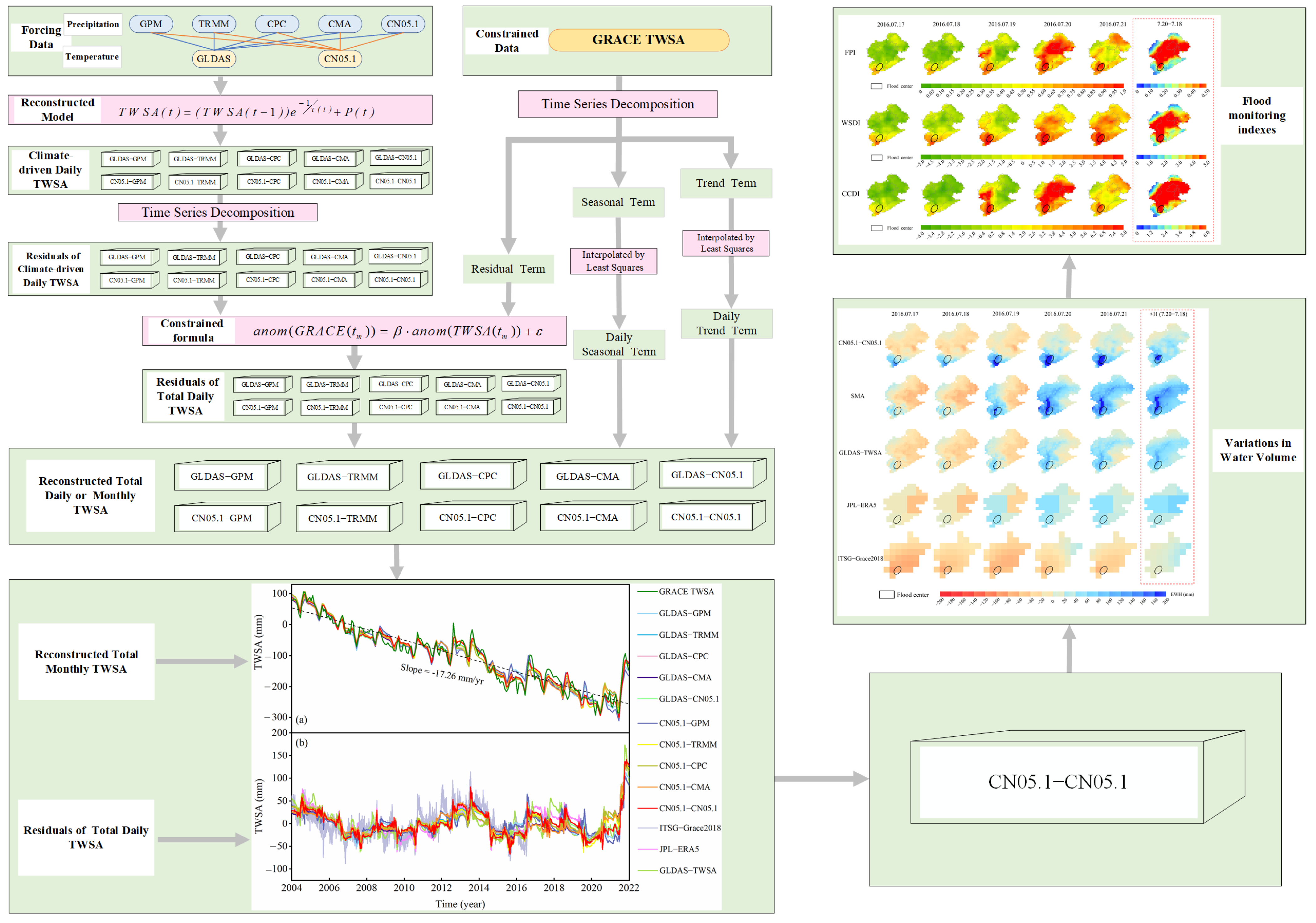
GLDAS does not have a clear vertical division for soil moisture, which is represented simply by the surface (0~2 cm), root zone (0~100 cm), and profile (varies grid-by-grid) reservoirs [56]. The sum of the three parts (SM) is treated as one of the auxiliary datasets. Additionally, the ITSG-Grace2018 provides the Kalman smoothed daily solutions [62,63], more importantly, it includes the same full hydrologic signal as the official GRACE monthly product [31]. The daily TWSA from GLDAS is included in the auxiliary datasets in addition to the JPL-ERA5 reconstructed by Humphrey and Gudmundsson [35]. It is worth noting that the average values from 2004 to 2009 have been removed from the above data to stay in step with TWSA. Therefore, these datasets are applied to evaluate the performance of reconstructed daily TWSA solutions, including soil moisture anomaly (SMA), ITSG-Grace2018, JPL-ERA5, and GLDAS-TWSA. Table 2 summarizes detailed information on the above datasets used in this study.

2.3. Methods

2.3.1. Reconstruction of Daily TWSA

GRACE-derived TWS changes are influenced by the combined effects of climate change and anthropogenic activities [64]. As the basic natural variables, precipitation and temperature can approximately represent the natural variability of global or regional TWS [65]. Inspired by the basic principles of hydrological modeling [35], Humphrey and Gudmundsson reconstructed the climate-driven daily TWSA by building a statistical model [66], which uses near real-time precipitation and temperature as input variables. Taking advantage of the relationship between the signals, this model is calibrated by GRACE TWSA to obtain the daily TWSA with total signal (for short TWSAtotal). Assuming a linear water storage model, water outputs are directly proportional to the storage and the residence time of the water store [66]. Based on this method, the model can be formulated as follow [35]:
T W S A ( t ) = ( T W S A ( t 1 ) ) e 1 τ ( t ) + P ( t ) ,
where P(t) and t denote the precipitation and daily time vector, respectively, τ(t) represents the residence time, and e−1/τ(t) is the consumption function of the water storage, which is related to temperature and ranges from 0 to 1. To ensure the accuracy of the reconstructed daily TWSA, the result of the model is further averaged into the “month scale”, and constrained by the GRACE TWSA, using the following formula [35]:
a n o m ( G R A C E ( t m ) ) = β a n o m ( T W S A ( t m ) ) + ε ,
where β is the constrained factor, which also can be called the calibrated parameter. The anom is the sign of the detrended and deseasonalized. tm and ε denote the monthly time vector and the error term, respectively. More details about the reconstruction can be found in Humphrey and Gudmundsson [35].

2.3.2. Time Series Decomposition

The anom processing in Equation (2) can be implemented through time series decomposition, and the time series of GRACE TWSA can be decomposed into the following series [45,67].
T W S A t o t a l = T W S A t r e n d + T W S A s e a s o n a l + T W S A r e s i d u a l ,
where TWSAtotal is the total signal, TWSAtrend and TWSAseasonal stand for liner trend and seasonal component, respectively. TWSAresidual represents the residual term, reflecting the inter-annual variation, sub-seasonal signal, and noise. Trends in TWSA largely reflect long-term changes in water depletion caused by human activities [68], and climate-driven inter-annual variation in TWSA is typically associated with floods in the mid- and low latitudes [69]. The high-frequency signals contained in the residual term may be closely related to short-term events. Therefore, the residual component is separated from the other components by the least squares method [70].
T W S A = a + b t + c cos ( 2 θ t ) + d sin ( 2 θ t ) + e cos ( 4 θ t ) + f sin ( 4 θ t ) + ε ,
where t means the time vector relative to 2004, a~f represents the parameters of each component, respectively. The ε is the same as in Equation (2) corresponding to TWSAresidual and a + b·t, and the remainder stand for the liner trend and seasonal components, which correspond to TWSAtrend and TWSAseasonal in Equation (3), separately. In addition, the trend and seasonal terms decomposed from the GRACE TWSA are interpolated by least squares to obtain the corresponding daily component, then the residual component is added to obtain daily TWSAtotal [38].

2.3.3. Flood Monitoring Indexes

Since the trend component of GRACE TWSA is mainly influenced by anthropogenic activities, the detrended TWSAtotal is extracted to calculate the daily flood monitoring indexes [71]. To express the potential to contain and stagnate floods, the TWSA and precipitation are chosen as input variables [24] and the FPI is calculated as follows:
F P A i , j = P i , j ( m a x ( T W S A i , j ) T W S A i , j 1 ) ,
F P I i , j = F P A i , j m i n ( F P A i , j ) m a x ( F P A i , j ) m i n ( F P A i , j ) ,
where i and j range from 2004 to 2021 and 1~365/366, which denote years and days respectively. TWSAi, j means the detrended TWSAtotal and Pi, j represents the precipitation. FPI emphasizes the probability of flooding under terrestrial saturation, and it implies a higher flood occurrence when FPI is closer to 1 [22]. Alternatively, other TWSA-based indexes such as WSDI and CCDI [26,72] are developed based on the standardization, and both are calculated using the following formulas:
P A i , j = P i , j m e a n ( P i , j ) ,
P A i , j R = P A i , j m e a n ( P A j ) ,
W S D i , j = T W S A i , j m e a n ( T W S A j ) ,
C C D i , j = W S D i , j + P A i , j R
W S D I i , j / C C D I i , j = W S D i , j / C C D i , j m e a n ( W S D i , j / C C D i , j ) s d ( W S D i , j / C C D i , j )
where PAi, j is the variation of precipitation relative to the average of the time series, PAj and TWSAj represent the collections of TWSA and PA on the same day in different years respectively. For example, when j = 1, the time collection corresponding to the variables includes 2004.01.01, 2005.01.01, 2006.01.01, ⋯⋯, and 2021.01.01. WSDi, j and CCDi, j are the water storage deficit and the combined climatologic deviation of the specific, respectively [73]. It is worth noting that WSDI and CCDI are calculated based on standardization, while the FPI is based on normalization, and different results are also caused by whether or not precipitation is considered. In addition, there is no clear grading about the relevant daily flood monitoring indexes, so the relative magnitude of the same index is treated as a reference value for flooding.

2.3.4. Evaluation Metrics

GRACE TWSA are utilized as references to assess the performance of reconstructed solutions. Three metrics are adopted to quantify the performance of reconstructed results, including the correlation coefficient (CC), root-mean-square error (RMSE), and Nash-Sutcliffe efficiency (NSE) coefficient. Detailed processes are depicted as follows [74,75]:
C C = i = 1 n ( O i O ¯ ) ( M i M ¯ ) i = 1 n ( O i O ¯ ) 2 i = 1 n ( M i M ¯ ) 2 ,
R M S E = 1 n i = 1 n ( O i M i ) 2 ,
N S E = 1 i = 1 n ( M i O i ) 2 i = 1 n ( O i O ¯ ) 2 ,
where Oi is the GRACE TWSA or the daily TWSA products shown in Table 2. Mi represents the reconstructed TWSA, the overbar denotes the mean value, and i and n denote i-th month or day and the total number, respectively. This means that the reconstructed results show better performance when the value of RMSE is lower, or the value of CC or NSE is closer to 1 [37]. The overall flowchart of this study is presented in Figure 2.

3. Results

3.1. Comparisons of Different GRACE-Filled Solutions

Since there is a data gap between GRACE and GRACE-FO from July 2017 to May 2018, it cannot meet the requirement of continuous TWSA solutions from 2004 to 2021. Therefore, the nearly one-year gap will be filled using the solutions provided by previous studies [43,50,51,52], and an important step is evaluating the performance of different products to choose an optimal solution. As shown in Figure 3, the Taylor diagrams illustrate the relationship between reconstructed TWSA and original CSR and JPL solutions. Both RMSE and CC metrics perform satisfactorily, with values of 20~30 mm and above 0.93 from January 2004 to June 2017, respectively (Figure 3a,c). As shown in Figure 3b, the red rectangle represented by BF is the closest to the original CSR solution, with the highest CC and the lowest RMSE of (0.50 and 27.77 mm). Similarly, the best performance is evaluated against the original JPL solution with CC and RMSE of (0.71 and 26.90 mm) (Figure 3d), which means that BF-based results perform best with GRACE-FO TWSA in the HRB. In addition, the time series of different products are illustrated in Figure 3e, and the BF-based results display good overall consistency with the original solutions in the HRB, especially during the GRACE-FO period. Thus, the BF-based reconstructed TWSA is chosen to fill the gap from July 2017 to May 2018 in this study.

3.2. Comparisons of Different Meteorological Products

Different daily precipitation and temperature products are compared from 2004 to 2021, and the results are shown in Figure 4 and Figure 5. As shown in Figure 4a, five kinds of precipitation products display similar seasonal variability, with the maximum rainfall occurring in June~October and the minimum during December~March. Moreover, these products have the same response to extreme rainfall, such as the maximums in 2012, 2016, and 2021. The difference is that outstanding performance in the multi-annual maximum is attained by CPC, while CN05.1 takes the maximum value of precipitation in 2016 and 2021. The CC and RMSE metrics are evaluated during the study period (Figure 4b,c). The heatmaps suggest that good consistency is observed between GPM and TRMM, CMA and CN05.1 with the CC and RMSE values of (0.92, 1.37 mm) and (0.90, 1.58 mm), respectively. However, the precipitation products provided by CN05.1 and CMA show poor agreement against GPM and TRMM with the CC below 0.73 and RMSE above 2.55 mm. As for the temperature, GLDAS and CN05.1 reach maximum values in July~August in the HRB. Additionally, the daily average values of GLADS and CN05.1 are 11.68 °C and 10.01 °C, and the former is slightly larger in amplitude than the latter, as shown in Figure 5. Moreover, the statistical distribution characteristics of the data are provided in Figures S1–S3 in the Supporting Information.

3.3. Evaluations of the Reconstructed TWSA Solutions

Different temperature and precipitation products are merged randomly, producing ten kinds of combinations, which include GLDAS-GPM, GLDAS-TRMM, GLDAS-CPC, GLDAS-CMA, GLDAS-CN05.1, CN05.1-GPM, CN05.1-TRMM, CN05.1-CPC, CN05.1-CMA, and CN05.1-CN05.1. Figure 6a presents the time series between reconstructed TWSA and GRACE TWSA at a monthly scale from January 2004 to December 2021. A remarkable downtrend is observed at the rate of −17.26 mm/year for monthly TWSA in the entire HRB. Better agreement is observed between GRACE TWSA and reconstructed TWSA with the NSE of 0.93~0.96, and the highest NSE is obtained by CN05.1-CN05.1 (Table 3). Notably, the GRACE TWSA in Table 3 stands for the average of CSR and JPL solution, which has been filled by the BF-based TWSA, and the reconstructed TWSA represents the reconstructed monthly TWSAtotal or daily TWSAresidual based on ten kinds of combinations.
From the perspective of daily scale, TWSAresidual based on different combinations present similar daily variations, which show the agreement with the NSE of 0.40 ~ 0.81 in the HRB against other daily TWSA including ITSG-Grcae2018, JPL-ERA5, and GLDAS-TWSA. A clear oscillation is shown in ITSG-Grace2018 (Figure 6b). Similarly, the CN05.1-CN05.1 performs best with the NSE of 0.52 ~ 0.81 from 2004 to 2021. It is worth noting that the precipitation may contribute more to the model than to temperature. As can be seen from Table 3, there are little differences in NSE when the same precipitation products are used, while significant differences are indicated between different combinations, which include the same temperature and different precipitation. For example, GLDAS-CN05.1 and CN05.1-CN05.1 show similar maximum NSE of 0.80 and 0.81, yet the maximum value of NSE for GLDAS-CMA is merely 0.60. In addition, the uncertainty based on Tricorn Hat Method (THM) [76] as well as CC and RMSE metrics are used to evaluate reconstructed TWSA in addition to NSE, which highlights the superiority of CN05.1-CN05.1 among the ten kinds of reconstructed results. In conclusion, the CN05.1-CN05.1 combination is chosen to reconstruct the grids within the HRB due to its better performance on the monthly and daily scales, and more comparison results are provided in Tables S1–S3 in the Supporting Information.

4. Discussions

4.1. Evolution of the Rainfall Process

It is reported that the rainfall gradually increased from 17 July to 18 July 2016, and reached its peak on 19 July, with the maximum precipitation over 600 mm at multiple local points (http://www.gov.cn/xinwen/2016-07/21/content_5093878.htm, accessed on 10 June 2022). The Haihe Water Conservancy Commission issued continuous flood warnings (http://www.hwcc.gov.cn/wwgj/haiweiyw/201607/t20160719_56444.html, accessed on 10 June 2022) and subsequently declared the first flood event in 2016. This flood caused huge economic losses in Hebei, Henan, Beijing, and Tianjin within the HRB as recorded by the “2016 Bulletin of Flood and Drought Disasters in China” [77].
To further understand the process of rainfall, the GPM precipitation data is used to depict the daily rainfall distribution map with a spatial resolution of 0.1° × 0.1° from 17 July to 21 July. As shown in Figure 7, the precipitation space moves from southwest to northeast, covering almost the whole basin. The plains area in front of the mountain is treated as a flood center including counties or districts of Anyang, Handan, and Xingtai, which was seriously damaged according to the “2016 Bulletin of Water Resources in Hebei and Anyang” [78,79].

4.2. Application of the Reconstructed daily TWSA

The detection of water volume change is essential for understanding and predicting flood events [4]. To evaluate the performance of the reconstructed daily TWSA, the reconstructed daily TWSA based on CN05.1-CN05.1 is used to evaluate water volume change during the 2016 short-term flood event. Figure 8a shows the residual variations of different products in the flood center, and it can be seen that reconstructed daily TWSA exhibits the strongest reaction with a maximum value of 216.19 mm. Figure 8b intuitively displays the specific change values from 18 July to 20 July, and the reconstructed daily TWSA rises by 168.83 mm in EWH during this period, followed by SMA and GLDAS-TWSA at 154.44 mm and 82.86 mm. Correspondingly, JPL-ERA5 and ITSG-Grace2018 perform poorly, with only 37.56 mm and 7.73 mm.
The spatial distribution of EWH is further shown in Figure 9. It can be seen that CN05.1-CN05.1, GLDAS-TWSA, and SMA are all able to track the movement of gridded precipitation and react to it in a timely manner from 17 July to 21 July, while JPL-ERA5 and ITSG-Grace2018 fail to work. The spatial distribution maps of increased EWH for different products are shown inside the red frame from July 18 to July 20. Similar to the change of time series in Figure 8, only CN05.1-CN05.1, SMA, and GLDAS-TWSA observably increase in the flood center. Although the SMA is larger than CN05.1-CN05.1 and GLDAS-TWSA, the reconstructed daily TWSA is stronger in the flood center from the view of responding to water volume change. In brief, compared to other daily products, reconstructed daily TWSA can sensitively capture the information on water volume changes caused by extreme rainfall, and perform a better response in time and space. That means the reconstructed daily TWSA possesses a crucial feature for monitoring flood events.

4.3. Spatiotemporal Analysis of the Short-Term Flood Event in 2016

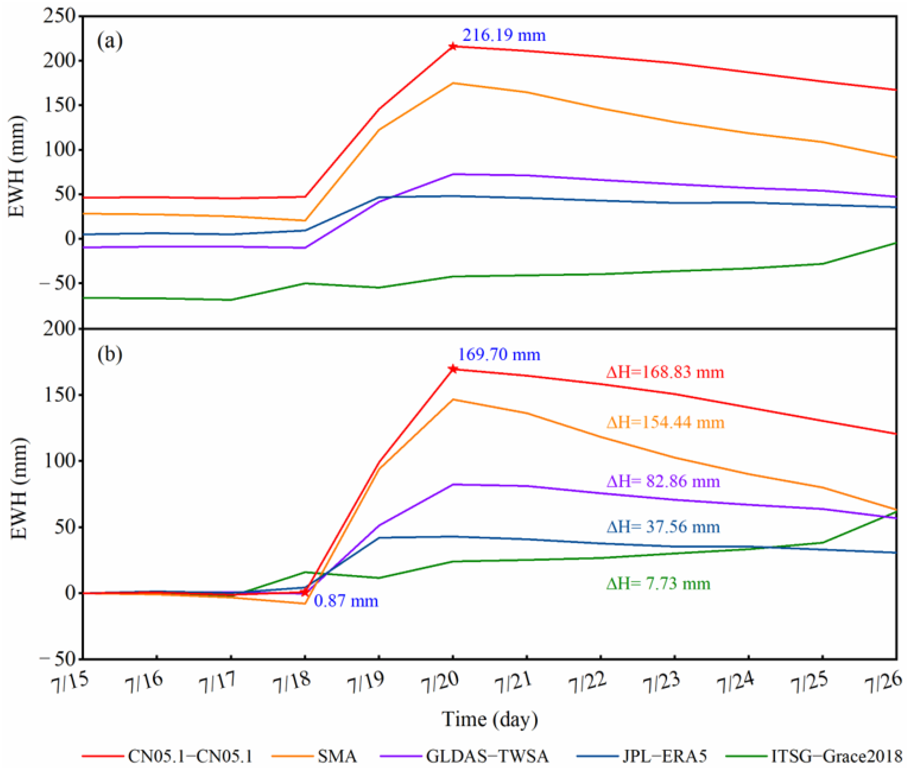
4.3.1. Temporal Variation of the Flood

To verify the accuracy of reconstructed results, three kinds of indexes based on reconstructed daily TWSA are constructed with the temporal and spatial resolutions selected as daily and 0.25° × 0.25°, including FPI, WSDI, and CCDI. The spatiotemporal evolution of the 2016 short-term flood event is evaluated by these indexes, and Figure 10 shows the temporal variation of FPI, WSDI, and CCDI from 1 January 2004 to 31 December 2021. Obviously, the three indexes accurately evaluate flood events that occurred in the HRB in 2012, 2016, and 2021, which are marked in gray. WSDI is consistent with FPI and CCDI in the description of flood in HRB, with similar peaks and troughs. It indicates that the flood indexes based on reconstructed daily TWSA have shown great potential for monitoring flood events in the basin. However, since these daily indexes are developed with different variables and approaches, FPI, CCDI, and WSDI differ in magnitude. For instance, compared to FPI and CCDI in the 2016 flood event, WSDI calculated only by TWSA does not respond significantly in its own range.

4.3.2. Spatial Distribution of the Flood

Figure 11 shows the spatial distribution of FPI, WSDI, and CCDI from 17 July to 21 July in 2016. Three daily indexes reveal the process of flood spreading from the southwest to the northeast, which is consistent with the record of the government-issued “2016 Bulletin of Flood and Drought Disasters in China” [77]. In addition, the spatial evolutions of FPI and CCDI are very similar and perform more significantly than WSDI in the entire basin, which corresponds to the temporal variation. Specifically, the three indexes are similar in the spatial scale on 17 and 18 July, foreshadowing flood events only in the south of the basin. Nevertheless, the difference between WSDI and other indexes becomes apparent from 19 July, and precipitation contributes markedly to FPI and CCDI as seen on 20 and 21 July.
To present the coverage of damage during the short-term flood, the increase of three indexes is evaluated as shown in the red frame from July 18 to July 20. In line with FPI and CCDI, this flood event is also detected by WSDI, which shows that the short-term flood has damaged the coastal area in western Liaoning province (http://www.gov.cn/xinwen/2016-07/21/content_5093443.htm, accessed on 12 June 2022) and most regions of Hebei province [78]. More specifically, the (number of the red grids/number of total grids) × 100% is utilized to simply quantify the proportion of area damaged by flooding in the HRB. Obviously, the severity of this flood may have been overestimated by the FPI and CCDI, both of which show flooding spreading to Chengde in the northern HRB with values of 56% and 66%, respectively. Unfortunately, this phenomenon is less consistent with the records of the “2016 Bulletin of Water Resources in Chengde” [80], which highlights that there was no flood in Chengde and that only the east of the city was disturbed by the rainstorm. In contrast to FPI and CCDI, the spatial distribution of WSDI matches well with the in situ records of the Water Resources Bulletins, and the quantified results show that 48% of the basin was damaged by this flood.

4.4. Response of Different Components of Soil Moisture in the Flood Event

Extreme climate change is easily understood through soil moisture, which usually contains several components with various depths [81]. Figure 12 displays the variation of three parts of soil moisture in the flood center from 15 July to 26 July 2016. It is obvious that great changes have taken place in the soil moisture profile with inter-day variation values of 52.46 mm and 31.92 mm from 18 July to 20 July, as well as changes in root zone soil moisture. It is noted that the greatest decline of EWH is observed in the root zone since the flood gradually recedes on 21 July, indicating that the damage from this flood occurred mainly in the root zone. This flood destroyed different parts of the soil with varying degrees, which poses a challenge for soil restoration in the future.

5. Conclusions

In order to overcome the shortcomings of the rough temporal resolution of GRACE TWSA, this study constructs three daily flood monitoring indexes based on reconstructed daily TWSA. Near real-time “Temperature-Precipitation” combinations are input into a statistical model to reconstruct the daily TWSA from 2004 to 2021, and the daily TWSA reconstructed by the best solution is then compared with other daily products in EWH. What is more, the daily TWSA-based FPI, WSDI, and CCDI are used to evaluate the short-term flood event in temporal evolution and spatial distribution. The primary conclusions are summarized:
  • Compared to the GRACE TWSA and other daily TWSA products, daily TWSA reconstructed based on CN05.1-CN05.1 perform best with the NSE of 0.96 and 0.52 ~ 0.81 among the ten combinations. The daily TWSA reconstructed by CN05.1-CN05.1 better reflects the dramatic increase of EWH than GLDAS-TWSA, JPL-ERA5, and ITSG-Grace2018 during the 2016 short-term flood event. In addition, the precipitation variable may contribute more to the model than temperature by comparing different reconstructed results.
  • Three daily flood monitoring indexes developed by reconstructed daily TWSA identify three recorded significant flood events in July 2012, July 2016, and July~October 2021 in the HRB. Moreover, FPI, WSDI, and CCDI reveal the fact that the spatial distribution in the 2016 short-term flood event extends from the southwest to the northeast, which is consistent with the track of the rainfall center. The spatiotemporal performance of FPI, WSDI, and CCDI validates the effectiveness of the daily flood monitoring indexes, which greatly improves the temporal characterization of flood monitoring.
  • During the 2016 short-term flood event, FPI and CCDI may have spatially overestimated the damage coverage of the flood with values of 56% and 66%, respectively. Importantly, the spatial impact of the flood assessed by WSDI is more consistent with the government report, and the quantified results show that 48% of the basin is damaged by the flood. Moreover, different parts of SM are compared, indicating the damage of this flood occurred mainly in the root zone. This paper not only contributes a method to GRACE TWSA for monitoring short-term flood events but also provides a potential reference for TWSA to be applied to short-term studies in more fields (e.g., sub-monthly evolution of drought and crustal movement). Notably, limited by input variables, the methodology is only applicable to areas where rainfall and temperature are the main factors affecting TWSA.

Supplementary Materials

The following are available online at https://www.mdpi.com/article/10.3390/rs15061564/s1, Figure S1: Statistical distribution of different rainfall products in Haihe River Basin from 1, January 2004 to 31 December 2021. Figure S2: Statistical distribution of the temperature from CN05.1 and GLDAS in the Haihe River Basi. Figure S3: Statistical distribution of the daily TWSA products in the Haihe River Basin. Table S1: CC, NSE and RMSE values between reconstructed monthly TWSAtotal and GRACE TWSA. Table S2: CC, NSE and RMSE values between reconstructed daily TWSA and Daily TWSA products at residual term. Table S3: Uncertainty among the reconstructed monthly TWSAtotal and daily TWSAresidual.

Author Contributions

S.N., W.Z., W.Y., Y.Z., Y.S. and K.L. collaborated to conduct this study; S.N.: scientific analysis, manuscript writing, and editing. W.Z. and W.Y.: experiment design, project management, review, and editing. Y.S. and Y.Z. and K L: review and editing. S.N. and W.Y.: processing of data. All authors contributed to the article and approved the submitted version. All authors have read and agreed to the published version of the manuscript.

Funding

This research was supported in part by the National Natural Science Foundation of China under Grant (42274119), in part by the Liaoning Revitalization Talents Program under Grant (XLYC2002082), in part by National Key Research and Development Plan Key Special Projects of Science and Technology Military Civil Integration (2022YFF1400500), and in part by the Key Project of Science and Technology Commission of the Central Military Commission.

Institutional Review Board Statement

Not applicable.

Informed Consent Statement

Not applicable.

Data Availability Statement

No new data were created or analyzed in this study. Data sharing is not applicable to this article.

Acknowledgments

The authors greatly appreciate the Climate Change Research Center, Chinese Academy of Science (https://ccrc.iap.ac.cn/, accessed on 13 July 2022) for the CN05.1 dataset and the institutions of CSR (http://www.csr.utexas.edu/grace/, accessed on 1 June 2022) and JPL (https://grace.jpl.nasa.gov/, accessed on 1 June 2022) that provide the GRACE mascon data. The authors would like to thank NASA for providing the datasets of GLDAS, GPM, and TRMM (http://agdisc.gsfc.nasa.gov/, accessed on 13 March 2022). We are thankful for the CPC data provided by Physical Sciences Laboratory, NOAA (https://psl.noaa.gov/data/gridded/, accessed on 10 July 2022). We also thank the China Meteorological Administration (CMA: http://data.cma.cn/, accessed on 3 June 2022) for providing the precipitation data. Shengkun Nie, Wei Zheng, and Wenjie Yin contributed equally to this paper.

Conflicts of Interest

The authors declare no conflict of interest.

References

  1. Jongman, B.; Ward, P.J.; Aerts, J.C.J.H. Global exposure to river and coastal flooding: Long term trends and changes. Glob. Environ. Change 2012, 22, 823–835. [Google Scholar] [CrossRef]
  2. Xiong, J.; Wang, Z.; Guo, S.; Wu, X.; Yin, J.; Wang, J.; Lai, C.; Gong, Q. High effectiveness of GRACE data in daily-scale flood modeling: Case study in the Xijiang River Basin, China. Nat. Hazards 2022, 113, 507–526. [Google Scholar] [CrossRef]
  3. Pangali Sharma, T.P.; Zhang, J.; Khanal, N.R.; Nepal, P.; Pangali Sharma, B.P.; Nanzad, L.; Gautam, Y. Household Vulnerability to Flood Disasters among Tharu Community, Western Nepal. Sustainability 2022, 14, 12386. [Google Scholar] [CrossRef]
  4. Sun, Z.; Zhu, X.; Pan, Y.; Zhang, J. Assessing Terrestrial Water Storage and Flood Potential Using GRACE Data in the Yangtze River Basin, China. Remote Sens. 2017, 9, 1011. [Google Scholar] [CrossRef] [Green Version]
  5. Song, X.; Zhang, C.; Zhang, J.; Zou, X.; Mo, Y.; Tian, Y. Potential linkages of precipitation extremes in Beijing-Tianjin-Hebei region, China, with large-scale climate patterns using wavelet-based approaches. Theor. Appl. Climatol. 2020, 141, 1251–1269. [Google Scholar] [CrossRef]
  6. Huang, Z.; Jiao, J.J.; Luo, X.; Pan, Y.; Jin, T. Drought and Flood Characterization and Connection to Climate Variability in the Pearl River Basin in Southern China Using Long-Term GRACE and Reanalysis Data. J. Clim. 2021, 34, 2053–2078. [Google Scholar] [CrossRef]
  7. The Ministry of Water Resources of the People’s Republic of China. 2020 Bulletin of Flood and Drought Disasters in China. pp. 15–30. Available online: http://www.mwr.gov.cn/sj/tjgb/zgshzhgb/202112/t20211208_1554245.html (accessed on 10 May 2022).
  8. Hagen, E.; Lu, X.X. Let us create flood hazard maps for developing countries. Nat. Hazards. 2011, 58, 841–843. [Google Scholar] [CrossRef]
  9. Burgan, H.I.; Icaga, Y. Flood analysis using Adaptive Hydraulics (AdH) model in Akarcay Basin. Tek. Dergi. 2019, 30, 9029–9051. [Google Scholar] [CrossRef] [Green Version]
  10. De Almeida, G.A.M.; Bates, P.; Ozdemir, H. Modelling urban floods at submetre resolution: Challenges or opportunities for flood risk management? J. Flood Risk Manag. 2018, 11, S855–S865. [Google Scholar] [CrossRef] [Green Version]
  11. Carreño Conde, F.; De Mata Muñoz, M. Flood Monitoring Based on the Study of Sentinel-1 SAR Images: The Ebro River Case Study. Water 2019, 11, 2454. [Google Scholar] [CrossRef] [Green Version]
  12. Tellman, B.; Sullivan, J.A.; Kuhn, C.; Kettner, A.J.; Doyle, C.S.; Brakenridge, G.R.; Erickson, T.A.; Slayback, D.A. Satellite imaging reveals increased proportion of population exposed to floods. Nature 2021, 596, 80–86. [Google Scholar] [CrossRef] [PubMed]
  13. Jiang, D.; Wang, J.; Huang, Y.; Zhou, K.; Ding, X.; Fu, J. The Review of GRACE Data Applications in Terrestrial Hydrology Monitoring. Adv. Meteorol. 2014, 2014, 1–9. [Google Scholar] [CrossRef] [Green Version]
  14. Grillakis, M.G.; Koutroulis, A.G.; Komma, J.; Tsanis, I.K.; Wagner, W.; Blöschl, G. Initial soil moisture effects on flash flood generation—A comparison between basins of contrasting hydro-climatic conditions. J. Hydrol. 2016, 541, 206–217. [Google Scholar] [CrossRef]
  15. Wasko, C.; Nathan, R.; Peel, M.C. Changes in Antecedent Soil Moisture Modulate Flood Seasonality in a Changing Climate. Water Resour. Res. 2020, 56, e2019WR026300. [Google Scholar] [CrossRef]
  16. Tapley, B.D.; Bettadpur, S.; Ries, J.C.; Thompson, P.F.; Watkins, M.M. GRACE measurements of mass variability in the Earth system. Science 2004, 305, 503–505. [Google Scholar] [CrossRef] [Green Version]
  17. Wahr, J.; Swenson, S.; Zlotnicki, V.; Velicogna, I. Time-variable gravity from GRACE: First results. Geophys. Res. Lett. 2004, 31, L11501. [Google Scholar] [CrossRef] [Green Version]
  18. Zheng, W.; Hsu, H.; Zhong, M.; Yun, M. Requirements Analysis for Future Satellite Gravity Mission Improved-GRACE. Surv. Geophys. 2015, 36, 87–109. [Google Scholar] [CrossRef]
  19. Chen, J.L.; Wilson, C.R.; Tapley, B.D. The 2009 exceptional Amazon flood and interannual terrestrial water storage change observed by GRACE. Water Resour. Res. 2010, 46, 12. [Google Scholar] [CrossRef] [Green Version]
  20. Tapley, B.D.; Bettadpur, S.; Watkins, M.; Reigber, C. The gravity recovery and climate experiment: Mission overview and early results. Geophys. Res. Lett. 2004, 31, L9607. [Google Scholar] [CrossRef] [Green Version]
  21. Rodell, M.; Velicogna, I.; Famiglietti, J.S. Satellite-based estimates of groundwater depletion in India. Nature 2009, 460, 999–1002. [Google Scholar] [CrossRef] [PubMed] [Green Version]
  22. Reager, J.T.; Famiglietti, J.S. Global terrestrial water storage capacity and flood potential using GRACE. Geophys. Res. Lett. 2009, 36, 23. [Google Scholar] [CrossRef] [Green Version]
  23. Zhou, I. Performance Evaluation of a Potential Component of an Early Flood Warning System—A Case Study of the 2012 Flood, Lower Niger River Basin, Nigeria. Remote Sens. 2019, 11, 1970. [Google Scholar]
  24. Xiong, J.; Wang, Z. Exploration of large-scale flood monitoring in the Pearl River basin based on GRACE satellites. J. Hydroelectr. Eng. 2021, 40, 68–78. [Google Scholar]
  25. Long, D.; Shen, Y.; Sun, A.; Hong, Y.; Longuevergne, L.; Yang, Y.; Li, B.; Chen, L. Drought and flood monitoring for a large karst plateau in Southwest China using extended GRACE data. Remote Sens. Environ. 2014, 155, 145–160. [Google Scholar] [CrossRef]
  26. Sinha, D.; Syed, T.H.; Reager, J.T. Utilizing combined deviations of precipitation and GRACE-based terrestrial water storage as a metric for drought characterization: A case study over major Indian river basins. J. Hydrol. 2019, 572, 294–307. [Google Scholar] [CrossRef]
  27. Nigatu, Z.M.; Fan, D.; You, W.; Melesse, A.M. Hydroclimatic Extremes Evaluation Using GRACE/GRACE-FO and Multidecadal Climatic Variables over the Nile River Basin. Remote Sens. 2021, 13, 651. [Google Scholar] [CrossRef]
  28. Tayfur, G. Discrepancy precipitation index for monitoring meteorological drought. J. Hydrol. 2021, 597, 126174. [Google Scholar] [CrossRef]
  29. Agboma, C.O.; Yirdaw, S.Z.; Snelgrove, K.R. Intercomparison of the total storage deficit index (TSDI) over two Canadian Prairie catchments. J. Hydrol. 2009, 374, 351–359. [Google Scholar] [CrossRef]
  30. Xiao, C.; Zhong, Y.; Feng, W.; Gao, W.; Wang, Z.; Zhong, M.; Ji, B. Monitoring the catastrophic flood with GRACE-FO and near-real-time precipitation data in northern Henan Province of China in July 2021. IEEE J. Sel. Top. Appl. Earth Observ. Remote Sens. 2022, 16, 89–101. [Google Scholar] [CrossRef]
  31. Kurtenbach, E.; Eicker, A.; Mayer-Gürr, T.; Holschneider, M.; Hayn, M.; Fuhrmann, M.; Kusche, J. Improved daily GRACE gravity field solutions using a Kalman smoother. J. Geodyn. 2012, 59–60, 39–48. [Google Scholar] [CrossRef]
  32. Gouweleeuw, B.T.; Kvas, A.; Gruber, C.; Gain, A.K.; Mayer-Gürr, T.; Flechtner, F.; Güntner, A. Daily GRACE gravity field solutions track major flood events in the Ganges-Brahmaputra Delta. Hydrol. Earth Syst. Sci. 2018, 22, 2867. [Google Scholar] [CrossRef] [Green Version]
  33. Xiong, J.; Guo, S.; Abhishek; Li, J.; Yin, J. A Novel Standardized Drought and Flood Potential Index Based on Reconstructed Daily GRACE Data. J. Hydrometeorol. 2022, 23, 1419–1438. [Google Scholar] [CrossRef]
  34. Jiang, Z.; Hsu, Y.; Yuan, L.; Huang, D. Monitoring time-varying terrestrial water storage changes using daily GNSS measurements in Yunnan, southwest China. Remote Sens. Environ. 2021, 254, 112249. [Google Scholar] [CrossRef]
  35. Humphrey, V.; Gudmundsson, L. GRACE-REC: A reconstruction of climate-driven water storage changes over the last century. Earth Syst. Sci. Data 2019, 11, 1153–1170. [Google Scholar] [CrossRef] [Green Version]
  36. Liu, B.; Zou, X.; Yi, S.; Sneeuw, N.; Cai, J.; Li, J. Identifying and separating climate- and human-driven water storage anomalies using GRACE satellite data. Remote Sens. Environ. 2021, 263, 112559. [Google Scholar] [CrossRef]
  37. Yang, X.; Tian, S.; You, W.; Jiang, Z. Reconstruction of continuous GRACE/GRACE-FO terrestrial water storage anomalies based on time series decomposition. J. Hydrol. 2021, 603, 127018. [Google Scholar] [CrossRef]
  38. Bai, H.; Ming, Z.; Zhong, Y.; Zhong, M.; Kong, D.; Ji, B. Evaluation of evapotranspiration for exorheic basins in China using an improved estimate of terrestrial water storage change. J. Hydrol. 2022, 610, 127885. [Google Scholar] [CrossRef]
  39. Hu, S.; Wang, Z.; Lee, J.H.W. Flood control and shrinkage in the Haihe River Mouth. Sci. China Ser. B Chem. 2001, 44, 240–248. [Google Scholar] [CrossRef]
  40. Zhang, G.; Zheng, W.; Yin, W.; Lei, W. Improving the Resolution and Accuracy of Groundwater Level Anomalies Using the Machine Learning-Based Fusion Model in the North China Plain. Sensors 2021, 21, 46. [Google Scholar] [CrossRef]
  41. Wang, Q.; Zheng, W.; Yin, W.; Kang, G.; Zhang, G.; Zhang, D. Improving the Accuracy of Water Storage Anomaly Trends Based on a New Statistical Correction Hydrological Model Weighting Method. Remote Sens. 2021, 13, 3583. [Google Scholar] [CrossRef]
  42. Guo, Y.; Shen, Y. Quantifying water and energy budgets and the impacts of climatic and human factors in the Haihe River Basin, China: 1. Model and validation. J. Hydrol. 2015, 528, 206–216. [Google Scholar] [CrossRef]
  43. Zhong, Y.; Feng, W.; Humphrey, V.; Zhong, M. Human-Induced and Climate-Driven Contributions to Water Storage Variations in the Haihe River Basin, China. Remote Sens. 2019, 11, 3050. [Google Scholar] [CrossRef] [Green Version]
  44. Haihe River Water Conservancy Commission. MWR. 2012 Bulletin of Water Resources in Haihe River Basin. Available online: http://www.hwcc.gov.cn/hwcc/static/szygb/gongbao2012/index.htm (accessed on 11 May 2022).
  45. Scanlon, B.R.; Zhang, Z.; Save, H.; Wiese, D.N.; Landerer, F.W.; Long, D.; Longuevergne, L.; Chen, J. Global evaluation of new GRACE mascon products for hydrologic applications. Water Resour. Res. 2016, 52, 9412–9429. [Google Scholar] [CrossRef] [Green Version]
  46. Zhang, L.; Sun, W. Progress and prospect of GRACE Mascon product and its application. Rev. Geophys. Planet. Phys. 2022, 53, 35–52. [Google Scholar]
  47. Save, H.; Bettadpur, S.; Tapley, B.D. High-resolution CSR GRACE RL05 mascons. J. Geophys. Res. Solid Earth 2016, 121, 7547–7569. [Google Scholar] [CrossRef]
  48. Wiese, D.N.; Landerer, F.W.; Watkins, M.M. Quantifying and reducing leakage errors in the JPL RL05M GRACE mascon solution. Water Resour. Res. 2016, 52, 7490–7502. [Google Scholar] [CrossRef]
  49. Chen, J. Satellite gravimetry and mass transport in the earth system. J. Geod. Geodyn. 2019, 10, 402–415. [Google Scholar] [CrossRef]
  50. Zhong, Y.; Feng, W.; Zhong, M.; Ming, Z. Dataset of Reconstructed Terrestrial Water Storage in China Based on Precipitation (2002–2019); National Tibetan Plateau/Third Pole Environment Data Center: Beijing, China, 2020. [Google Scholar] [CrossRef]
  51. Mo, S.; Zhong, Y.; Forootan, E.; Mehrnegar, N.; Yin, X.; Wu, J.; Feng, W.; Shi, X. Bayesian convolutional neural networks for predicting the terrestrial water storage anomalies during GRACE and GRACE-FO gap. J. Hydrol. 2022, 604, 127244. [Google Scholar] [CrossRef]
  52. Rateb, A.; Sun, A.; Scanlon, B.R.; Save, H.; Hasan, E. Reconstruction of GRACE Mass Change Time Series Using a Bayesian Framework. Earth Space Sci. 2022, 9, e2021EA002162. [Google Scholar] [CrossRef]
  53. Wu, T.; Zheng, W.; Yin, W.; Zhang, H. Spatiotemporal Characteristics of Drought and Driving Factors Based on the GRACE-Derived Total Storage Deficit Index: A Case Study in Southwest China. Remote Sens. 2021, 13, 79. [Google Scholar] [CrossRef]
  54. Huffman, G.J.; Stocker, E.F.; Bolvin, D.T.; Nelkin, E.J.; Tan, J. GPM IMERG Early Precipitation L3 1 Day 0.1 Degree × 0.1 Degree V06, Edited by Andrey Savtchenko, Greenbelt, MD, Goddard Earth Sciences Data and Information Services Center (GES DISC). 2019. Available online: https://disc.gsfc.nasa.gov/datasets/GPM_3IMERGDE_06/summary (accessed on 13 March 2022).
  55. Huffman, G.J.; Bolvin, D.T.; Nelkin, E.J.; Adler, R.F. TRMM (TMPA) Precipitation L3 1 Day 0.25 Degree × 0.25 Degree V7, Edited by Andrey Savtchenko, Goddard Earth Sciences Data and Information Services Center (GES DISC). 2016. Available online: https://disc.gsfc.nasa.gov/datasets/TRMM_3B42_Daily_7/summary (accessed on 13 March 2022).
  56. Li, B.; Beaudoing, H.; Rodell, M. NASA/GSFC/HSL, GLDAS Catchment Land Surface Model L4 Daily 0.25 × 0.25 Degree GRACE-DA1 V2.2, Greenbelt, Maryland, USA, Goddard Earth Sciences Data and Information Services Center (GES DISC). 2020. Available online: https://disc.gsfc.nasa.gov/datasets/GLDAS_CLSM025_DA1_D_2.2/summary (accessed on 15 May 2022).
  57. Xu, Y.; Gao, W.; Shen, Y.; Xu, C.; Shi, Y.; Giogri, F. A Daily Temperature Dataset over China and Its Application in Validating a RCM Simulation. Adv. Atmos. Sci. 2009, 4, 763–772. [Google Scholar] [CrossRef]
  58. Wu, J.; Gao, X. A gridded daily observation dataset over China region and comparison with the other datasets. Chinese J. Geophys. 2013, 56, 1102–1111. [Google Scholar]
  59. Sun, Q.; Miao, C.; Duan, Q.; Ashouri, H.; Sorooshian, S.; Hsu, K.L. A Review of Global Precipitation Data Sets: Data Sources, Estimation, and Intercomparisons. Rev. Geophys. 2018, 56, 79–107. [Google Scholar] [CrossRef] [Green Version]
  60. Yang, Y.; Shen, L.; Wang, B. How is the precipitation distributed vertically in arid mountain region of Northwest China? J. Geogr. Sci. 2022, 32, 241–258. [Google Scholar] [CrossRef]
  61. Contractor, S.; Donat, M.G.; Alexander, L.V.; Ziese, M.; Meyer-Christoffer, A.; Schneider, U.; Rustemeier, E.; Becker, A.; Durre, I.; Vose, R.S. Rainfall Estimates on a Gridded Network (REGEN)—A global land-based gridded dataset of daily precipitation from 1950 to 2016. Hydrol. Earth Syst. Sci. 2020, 24, 919–943. [Google Scholar] [CrossRef] [Green Version]
  62. Kvas, A.; Behzadpour, S.; Ellmer, M.; Klinger, B.; Strasser, S.; Zehentner, N.; Mayer Gürr, T. ITSG-Grace2018: Overview and Evaluation of a New GRACE-Only Gravity Field Time Series. J. Geophys. Res. Solid Earth 2019, 124, 9332–9344. [Google Scholar] [CrossRef] [Green Version]
  63. Mayer-Gürr, T.; Behzadpour, S.; Ellmer, M.; Kvas, A.; Klinger, B.; Strasser, S.; Zehentner, N. ITSG-Grace2018—Monthly, Daily and Static Gravity Field Solutions from GRACE. GFZ Data Serv. 2018. Available online: https://www.tugraz.at/institute/ifg/downloads/gravity-field-models/itsg-grace2018 (accessed on 18 July 2022).
  64. Long, D.; Pan, Y.; Zhou, J.; Chen, Y.; Hou, X.; Hong, Y.; Scanlon, B.R.; Longuevergne, L. Global analysis of spatiotemporal variability in merged total water storage changes using multiple GRACE products and global hydrological models. Remote Sens. Environ. 2017, 192, 198–216. [Google Scholar] [CrossRef]
  65. Humphrey, V.; Gudmundsson, L.; Seneviratne, S.I. A global reconstruction of climate-driven subdecadal water storage variability. Geophys. Res. Lett. 2017, 44, 2300–2309. [Google Scholar] [CrossRef]
  66. Beven, K.J. Rainfall-Runoff Modelling: The Primer, 2nd ed.; John Wiley & Sons: Chichester, UK, 2012. [Google Scholar]
  67. Humphrey, V.; Gudmundsson, L.; Seneviratne, S.I. Assessing Global Water Storage Variability from GRACE: Trends, Seasonal Cycle, Subseasonal Anomalies and Extremes. Surv. Geophys. 2016, 37, 357–395. [Google Scholar] [CrossRef] [Green Version]
  68. Long, D.; Scanlon, B.R.; Longuevergne, L.; Sun, A.Y.; Fernando, D.N.; Save, H. GRACE satellite monitoring of large depletion in water storage in response to the 2011 drought in Texas. Geophys. Res. Lett. 2013, 40, 3395–3401. [Google Scholar] [CrossRef] [Green Version]
  69. Tapley, B.D.; Watkins, M.M.; Flechtner, F.; Reigber, C.; Bettadpur, S.; Rodell, M.; Sasgen, I.; Famiglietti, J.S.; Landerer, F.W.; Chambers, D.P.; et al. ; et al. Contributions of GRACE to understanding climate change. Nat. Clim. Change 2019, 9, 358–369. [Google Scholar] [CrossRef]
  70. Jensen, L.; Eicker, A.; Dobslaw, H.; Stacke, T.; Humphrey, V. Long-Term Wetting and Drying Trends in Land Water Storage Derived From GRACE and CMIP5 Models. J. Geophys. Res. Atmos. 2019, 124, 9808–9823. [Google Scholar] [CrossRef] [Green Version]
  71. Xu, Y.; Zhu, X.; Cheng, X.; Gun, Z.; Lin, J.; Zhao, J.; Yao, L.; Zhou, C. Drought assessment of China in 2002–2017 based on a comprehensive drought index. Agric. For. Meteorol. 2022, 319, 108922. [Google Scholar] [CrossRef]
  72. Thomas, A.C.; Reager, J.T.; Famiglietti, J.S.; Rodell, M. A GRACE-based water storage deficit approach for hydrological drought characterization. Geophys. Res. Lett. 2014, 41, 1537–1545. [Google Scholar] [CrossRef] [Green Version]
  73. Xiong, J.; Yin, J.; Guo, S.; Gu, L.; Xiong, F.; Li, N. Integrated flood potential index for flood monitoring in the GRACE era. J. Hydrol. 2021, 603, 127115. [Google Scholar] [CrossRef]
  74. Nash, J.E.; Sutcliffe, J.V. River flow forecasting through conceptual models part I—A discussion of principles. J. Hydrol. 1970, 10, 282–290. [Google Scholar] [CrossRef]
  75. Yin, W.; Zhang, G.; Han, S.; Yeo, I.; Zhang, M. Improving the resolution of GRACE-based water storage estimates based on machine learning downscaling schemes. J. Hydrol. 2022, 613, 128447. [Google Scholar] [CrossRef]
  76. Ferreira, V.G.; Montecino, H.D.C.; Yakubu, C.I.; Heck, B. Uncertainties of the Gravity Recovery and Climate Experiment time-variable gravity-field solutions based on three-cornered hat method. J. Appl. Remote Sens. 2016, 10, 15015. [Google Scholar] [CrossRef]
  77. The Ministry of Water Resources of the People’s Republic of China. 2016 Bulletin of Flood and Drought Disasters in China. pp. 23–29. Available online: http://www.mwr.gov.cn/sj/tjgb/zgshzhgb/201707/t20170720_966705.html (accessed on 10 June 2022).
  78. The Department of Water Resoueces of Hebei Province, China. 2016 Bulletin of Water Resources in Hebei. Available online: http://slt.hebei.gov.cn/a/2018/03/02/2018030221906.html (accessed on 12 June 2022).
  79. The Bureau of Water Resources of Anyang City, Henan Province, China. 2016 Bulletin of Water Resources in Anyang. Available online: https://slj.anyang.gov.cn/2017/12-05/2254922.html (accessed on 12 June 2022).
  80. The Bureau of Water Resources of Chengde City, Hebei Province, China. 2016 Bulletin of Water Resources in Chengde. Available online: https://www.chengde.gov.cn/art/2018/10/11/art_9943_319281.html (accessed on 25 June 2022).
  81. Berghuijs, W.R.; Harrigan, S.; Molnar, P.; Slater, L.J.; Kirchner, J.W. The Relative Importance of Different Flood-Generating Mechanisms Across Europe. Water Resour. Res. 2019, 55, 4582–4593. [Google Scholar] [CrossRef] [Green Version]
Figure 1. Information of the Haihe River basin; (a) location; (b) elevation; (c) land cover in 2020; (d) distribution of meteorological stations.
Remotesensing 15 01564 g001
Figure 2. Flowchart of this study (The pink means method; Cuboids are the variable combinations; Ellipses stand for the data and pictures represent the results).
Remotesensing 15 01564 g002
Figure 3. Comparison of reconstructed monthly TWSA and GRACE TWSA; (a,b) CC and RMSE between reconstructed monthly TWSA and CSR solution during GRACE and GRACE-FO period; (c,d) CC and RMSE between reconstructed monthly TWSA and JPL solution during GRACE and GRACE-FO period; (e) Time series of the reconstructed monthly TWSA, CSR and JPL solution from 2004 to 2021.
Remotesensing 15 01564 g003
Figure 4. Performance of different precipitation products in the HRB from 2004 to 2021; (a) Time series of precipitation products; (b) CC values between precipitation products; (c) RMSE values between precipitation products.
Remotesensing 15 01564 g004
Figure 5. Different temperature variations in the HRB from 2004 to 2021.
Remotesensing 15 01564 g005
Figure 6. Comparations of reconstructed TWSA based on different precipitation and temperature; (a) Monthly TWSAtotal; (b) daily TWSAresidual.
Remotesensing 15 01564 g006
Figure 7. Spatial distribution of the rainfall from 17 July to 21 July 2016.
Remotesensing 15 01564 g007
Figure 8. Comparisons of residual items from CN05.1-CN05.1, GLDAS-TWSA, SMA, JPL-ERA5, and ITSG-Grace2018 in flood center; (a) Original variations, (b) variations relative to the same benchmark.
Remotesensing 15 01564 g008
Figure 9. The spatial distribution of reconstructed daily TWSA (0.25° × 0.25°) based on CN05.1-CN05.1, SMA (0.25° × 0.25°), GLDAS-TWSA (0.25° × 0.25°), JPL-ERA5 (0.5° × 0.5°), and ITSG-Grace2018 daily TWSA (1° × 1°) in July with the seasonal cycle and the linear trend removed.
Remotesensing 15 01564 g009
Figure 10. Temporal variations of FPI, WSDI, and CCDI from 1 January 2004 to 31 December 2021 in the HRB.
Remotesensing 15 01564 g010
Figure 11. The spatial distribution of FPI, WSDI, and CCDI from 18 July to 21 July in the HRB.
Remotesensing 15 01564 g011
Figure 12. Variation of different soil moistures in the flood center during the short-term flood.
Remotesensing 15 01564 g012
Table 1. Information of reconstructed TWSA products in previous studies.
DataTemporal ResolutionSpatial ResolutionTime SpanCoverSources
LPD_CSRmonthly0.25° × 0.25°April 2002~December 2019China[43,50]
LPD_JPLmonthly0.5° × 0.5°April 2002~December 2019China[43,50]
BCNNmonthly1° × 1°April 2002~August 2020Global[51]
BFmonthly1° × 1°April 2002~April 2021Global[52]
Table 2. Details of the different datasets used in this study.
DataShort NameTemporal ResolutionSpatial ResolutionTime Span
GRACE TWSACSRmonthly0.25° × 0.25°April 2002~January 2022
JPLmonthly0.5° × 0.5°April 2002~January 2022
Precipitation (PRE)GPMdaily0.1° × 0.1°1 June 2000~10 March 2022
TRMMdaily0.25° × 0.25°1 January 1998~1 January 2020
CPCdaily0.5° × 0.5°1 January 1979~11 March 2022
CMAdaily0.5° × 0.5°1 January 1961~31 December 2021
CN05.1daily0.25° × 0.25°1 January 1961~31 December 2021
GLDASdaily0.25° × 0.25°1 February 2003~18 January 2022
Temperature (Temp)GLDASdaily0.25° × 0.25°1 February 2003~18 January 2022
CN05.1daily0.25° × 0.25°1 January 1961~31 December 2021
Daily TWSAGLDAS-TWSAdaily0.25° × 0.25°1 February 2003~18 January 2022
JPL-ERA5daily0.5° × 0.5°1 January 1979~31 July 2019
ITSG-Grace2018daily1° × 1°1 April 2002~31 August 2016
Soil moisture anomaliesSMAdaily0.25° × 0.25°1 February 2003~18 January 2022
The GRACE data was accessed on 18 April 2022.
Table 3. NSE between the reconstructed TWSA and GRACE TWSA and daily TWSA products.
NSEGRACE TWSADaily TWSA Products
GLDAS-GPM0.940.40~0.60
GLDAS-TRMM0.960.50~0.75
GLDAS-CPC0.960.41~0.57
GLDAS-CMA0.950.49~0.60
GLDAS-CN05.10.960.50~0.80
CN05.1-GPM0.930.42~0.58
CN05.1-TRMM0.960.53~0.75
CN05.1-CPC0.960.42~0.58
CN05.1-CMA0.950.48~0.63
CN05.1-CN05.10.960.52~0.81
Disclaimer/Publisher’s Note: The statements, opinions and data contained in all publications are solely those of the individual author(s) and contributor(s) and not of MDPI and/or the editor(s). MDPI and/or the editor(s) disclaim responsibility for any injury to people or property resulting from any ideas, methods, instructions or products referred to in the content.

