Article

Water Stream Extraction via Feature-Fused Encoder-Decoder Network Based on SAR Images

1
College of Computer and Information Engineering, Henan University, Kaifeng 475004, China
2
Henan Engineering Research Center of Intelligent Technology and Application, Henan University, Kaifeng 475004, China
3
Henan Key Laboratory of Big Data Analysis and Processing, Henan University, Kaifeng 475004, China
4
Institute of Geographical Sciences, Henan Academy of Sciences, Zhengzhou 450052, China
5
Henan Key Laboratory of Remote Sensing and Geographic Information System, Zhengzhou 450052, China
*
Author to whom correspondence should be addressed.
Remote Sens. 2023, 15(6), 1559; https://doi.org/10.3390/rs15061559
Submission received: 4 February 2023 / Revised: 6 March 2023 / Accepted: 10 March 2023 / Published: 13 March 2023
(This article belongs to the Special Issue Remote Sensing Applications for the Biosphere)

Abstract

:
The extraction of water stream based on synthetic aperture radar (SAR) is of great significance in surface water monitoring, flood monitoring, and the management of water resources. However, in recent years, the research mainly uses the backscattering feature (BF) to extract water bodies. In this paper, a feature-fused encoder–decoder network was proposed for delineating the water stream more completely and precisely using both the BF and polarimetric feature (PF) from SAR images. Firstly, the standard BFs were extracted and PFs were obtained using model-based decomposition. Specifically, the newly model-based decomposition, more suitable for dual-pol SAR images, was selected to acquire three different PFs of surface water stream for the first time. Five groups of candidate feature combinations were formed with two BFs and three PFs. Then, a new feature-fused encoder–decoder network (FFEDN) was developed for mining and fusing both BFs and PFs. Finally, several typical areas were selected to evaluate the performance of different combinations for water stream extraction. To further verify the effectiveness of the proposed method, two machine learning methods and four state-of-the-art deep learning algorithms were utilized for comparison. The experimental results showed that the proposed method using the optimal feature combination achieved the highest accuracy, with a precision of 95.21%, recall of 91.79%, intersection over union (IoU) score of 87.73%, overall accuracy (OA) of 93.35%, and average accuracy (AA) of 93.41%. The results showed that the performance was higher when BF and PF were combined. In short, in this study, the effectiveness of PFs for water stream extraction was verified and the proposed FFEDN can further improve the accuracy of water stream extraction.

Graphical Abstract

1. Introduction

Surface water, including rivers, lakes, reservoirs, and ponds, generally has certain connectivity and forms a water stream [1]. Extracting the water stream accurately and completely can provide powerful data for surface water resources management and planning as well as drought and flood disaster prevention and control [2], which contributes to socio-economic development and ecological protection [3].
Nowadays, remote sensing technology is regarded as an efficient means for the investigation of surface water resources and has a high accuracy for the extraction of the water stream in large-scale images because it can make use of various features [4]. At present, optical remote sensing [5,6,7,8] and digital elevation models (DEMs) [9,10,11,12] obtained from different satellites have been widely used with a range of supervised and unsupervised methods [13]. However, the optical data can be prone to being affected by clouds, rain, and fogs, so it may not be possible to obtain high-quality images at the specific time [14]. Meanwhile, the methods using DEMs also have some problems such as low accuracy in extracting water bodies [15]. As a result, it is difficult to extract water body by using these data in specific area or time. Fortunately, synthetic aperture radar (SAR), as an active earth observation system, can detect targets at all times which are not affected by weather and meteorological factors and can detect targets at all times [16,17]. Water bodies have a lower scattering value and present as dark area in SAR images compared with other ground objects, which make it easy to extract surface water.
Based on these characteristics, scholars have put forward many different water extraction methods, including threshold segmentation [18,19], mathematical statistical algorithms [20], machine learning [21,22,23,24], and deep learning [25,26,27]. The threshold method determines whether the pixels are water bodies through a suitable preset threshold. This method is easy to implement, but the setting of suitable threshold is difficult to find [28]. The Wishart classifier utilizes polarimetric information to extract water bodies and has more accurate extraction results in small areas, but the spatial continuity is weak [29]. Machine learning methods, such as random forest (RF) [30], support vector machine (SVM) [31], and Markov random field (MRF) [32], require higher computing power and are always affected by speckle noise in SAR images, which lead to inaccurate extraction results. The above methods attempt to establish a mapping relationship to classify each pixel, which is difficult due to the influence of speckle noise [33]. In recent years, deep learning methods have overcome these problems because of their powerful feature extraction capabilities. Convolutional neural networks (CNN), such as U-Net, DeepLab, and others, have achieved remarkable results [34,35,36,37]. Nemni et al. used an improved U-Net to rapidly extract water bodies with VV polarization backscattering images of Sentinel-1 [38]. Based on the DeepLab model, Guo et al. established a new model to quickly extract flooded areas by using both VV and VH polarization backscattering images [39]. Xue et al., proposed dense-coordinate-feature-concatenate network (DCFNet) and combines the features of HH and HV polarization backscattering images [40]. Chen et al., proposed a model named MSF-MLSAN (multi-scale spatial feature-multi-level selective attention network) to extract a water body in backscattering images of millimeter-wave SAR data. [41]. Zhang et al., proposed a U-Net-based model, WENET, to extract the waterline from Sentinel-1 SAR images [42]. Baumhoer et al., used a U-Net model to extract the Antarctic coastline for tracking glacier and ice shelf front movement using Sentinel-1 data [43]. Combining the holistically-nested edge detection (HED) and U-Net, Heidler et al. recently successfully extracted the Antarctic coast’s waterline and completed the sea–land classification simultaneously for Sentinel-1 SAR imagery [44]. However, these deep learning methods were mainly focused on the backscattering features (BFs) and select one or multiple BFs as the input of the model; the polarimetric features (PFs) have not been utilized adequately.
This paper proposed a deep learning method, which fully integrated BFs and PFs, and whether the fused features can extract water stream more accurately from Sentinel-1A SAR images was discussed. First, the BFs of VV and VH were obtained and the PFs were gained using the model-based decomposition method. Then, a feature-fused encoder–decoder Network based on U-Net [45] was proposed for extracting and fusing valid water features from all of the above features to extract the water stream more precisely and connectively. The main contributions of this paper are:
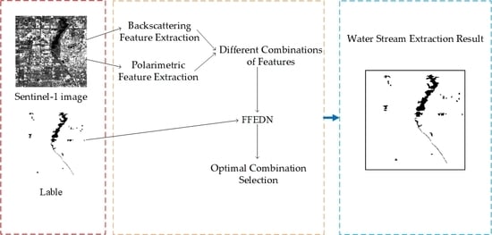
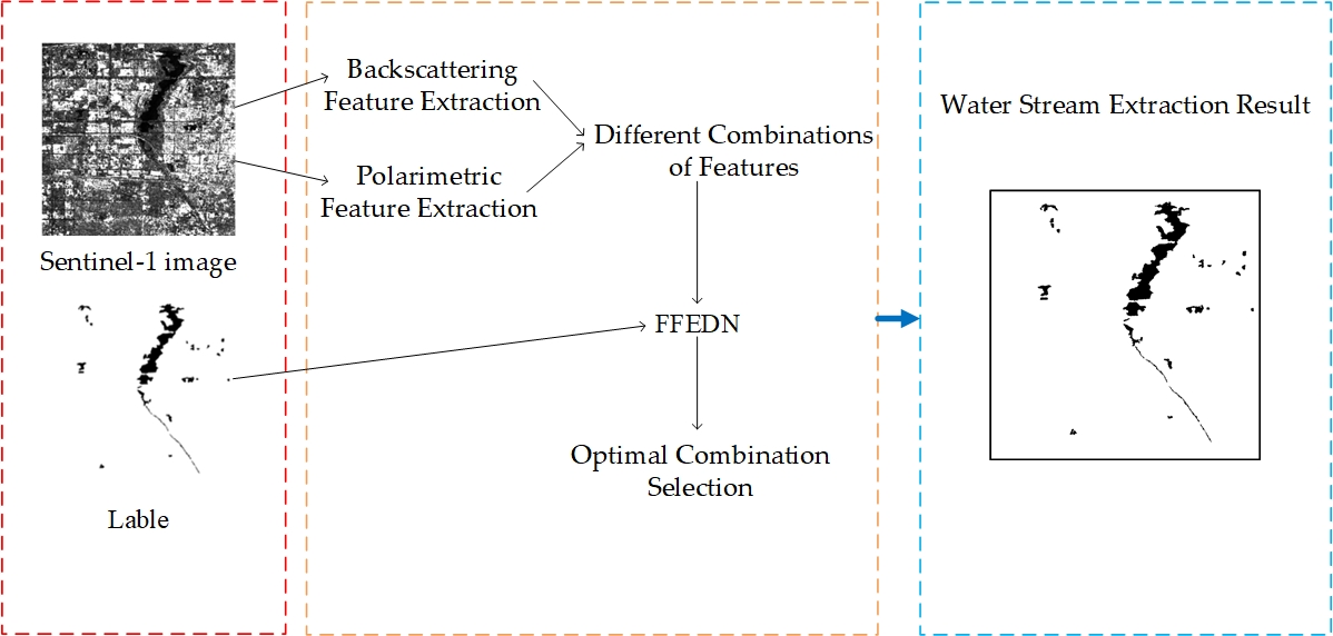
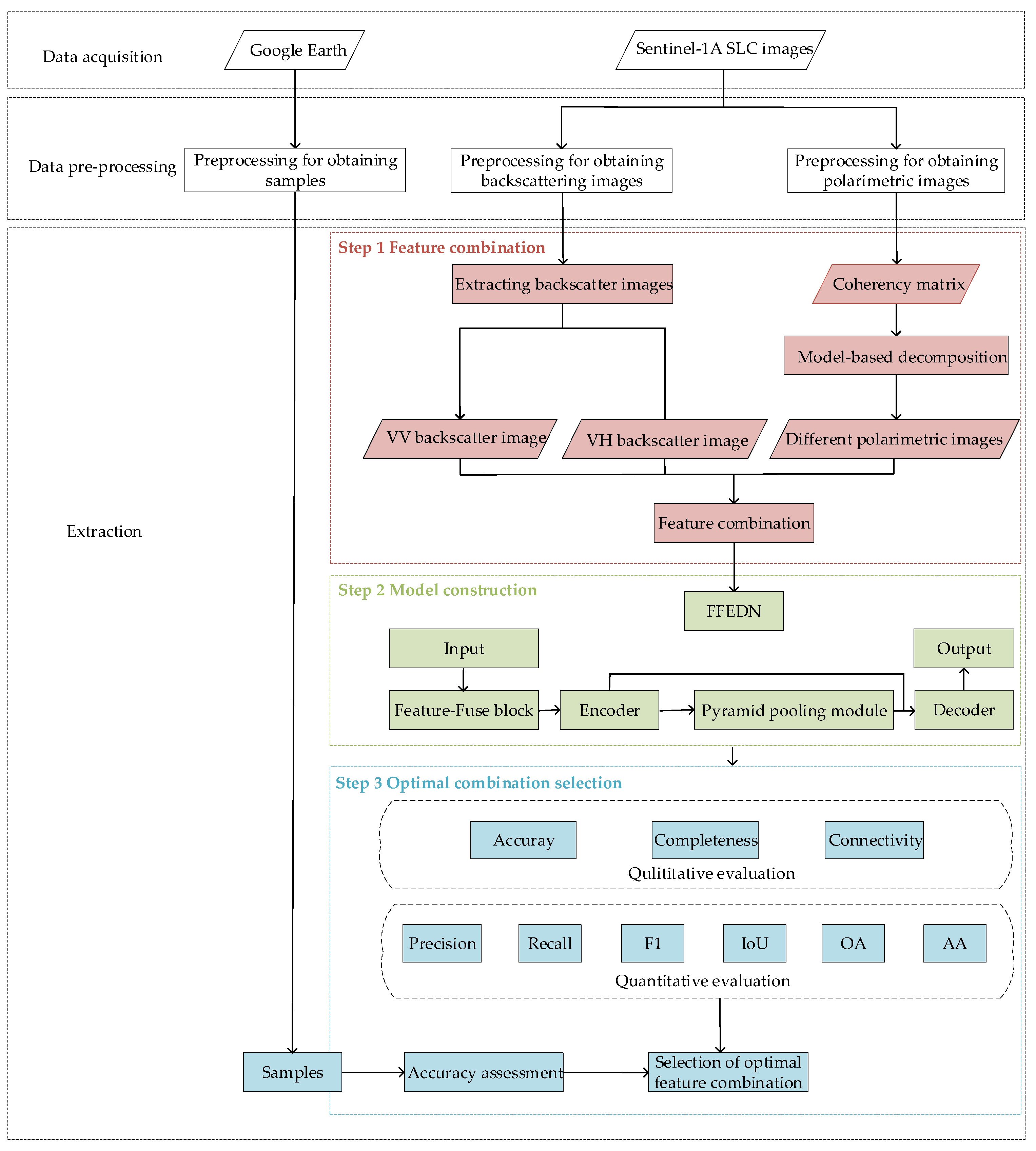
  • The water features from BFs and PFs are fully integrated by using feature-fused block and the influence of different combinations on water stream extraction is explored. Especially, the influence of PFs obtained by the newly model-based decomposition adapted to dual-pol SAR images was first discussed in the task of water stream extraction.
  • An effective water stream extraction model FFEDN is proposed. It has an outstanding capability of feature learning and feature fusing, which improves the extraction accuracy.
The rest of this paper is organized as follows. Section 2 describes the study area and datasets for data pre-processing, model training, and the accuracy assessment. Section 3 shows the results of extraction and Section 4 discusses the results as remaining limitations of our method. Finally, Section 5 summarizes the findings of this paper.

2. Materials and Methods
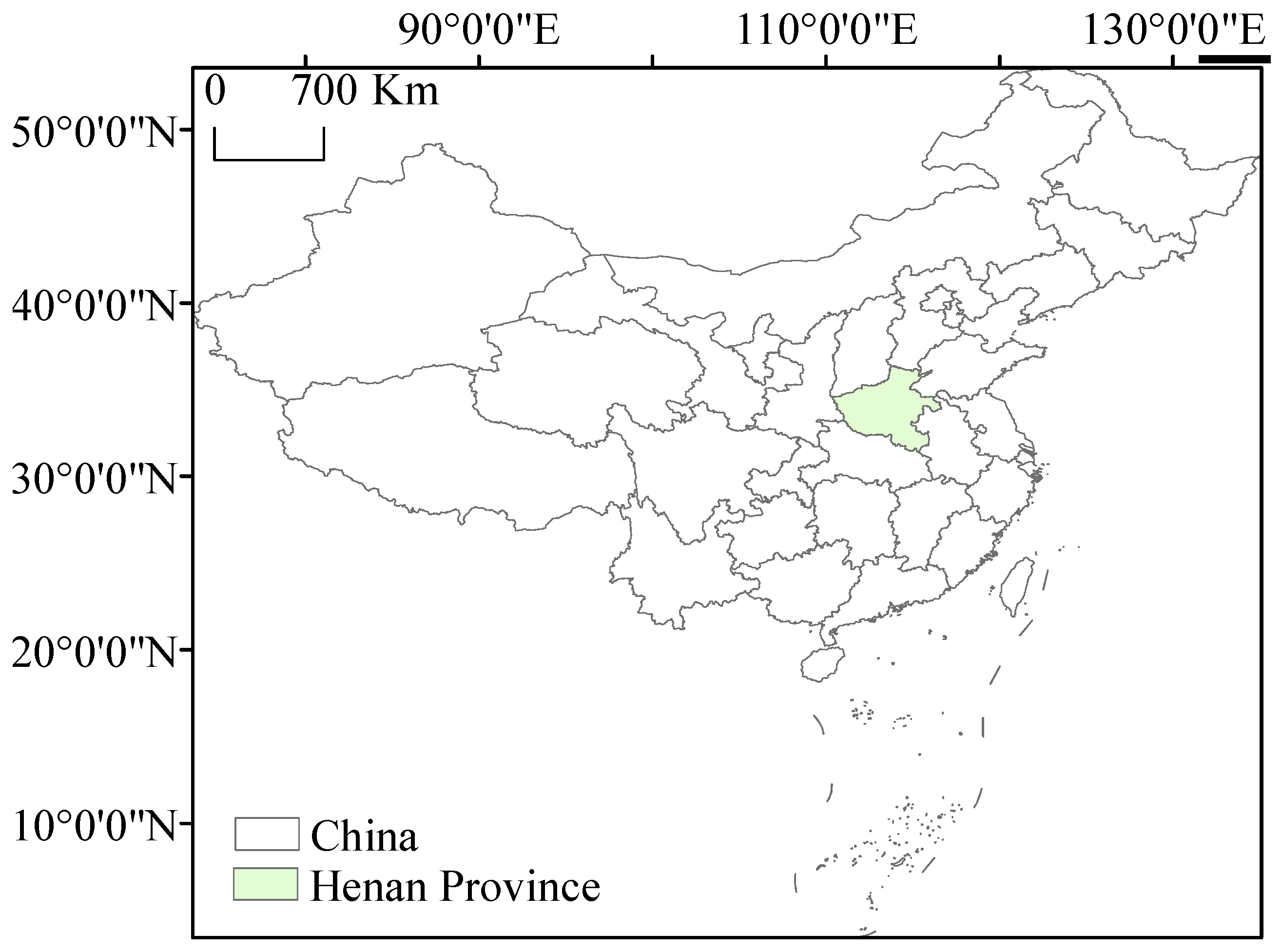
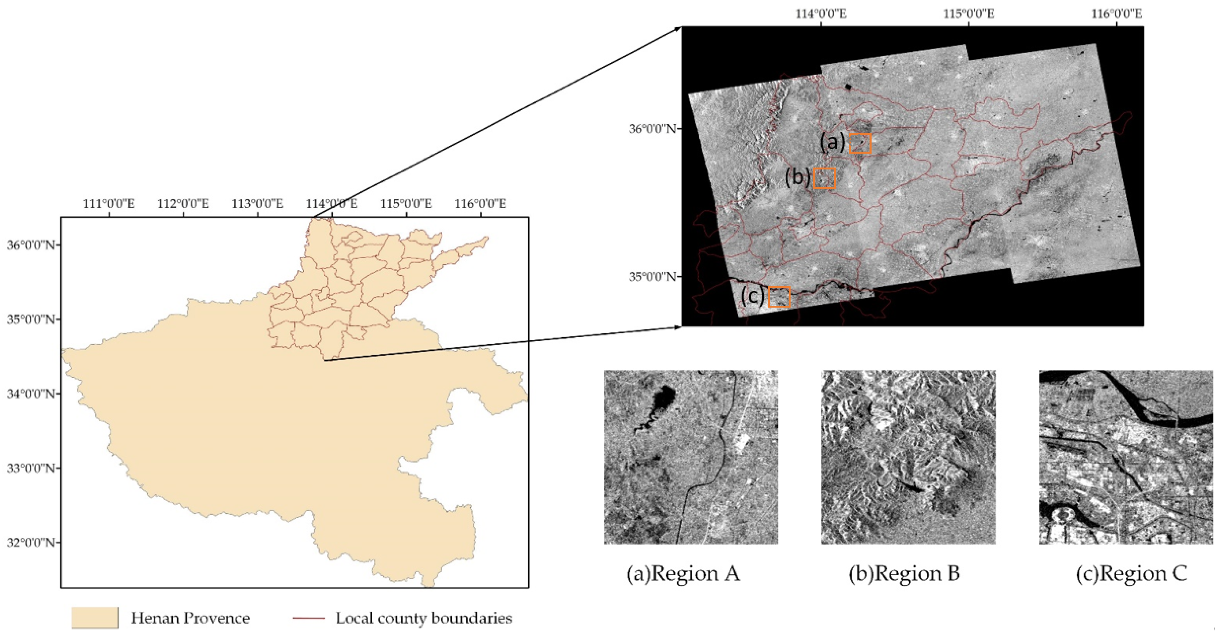
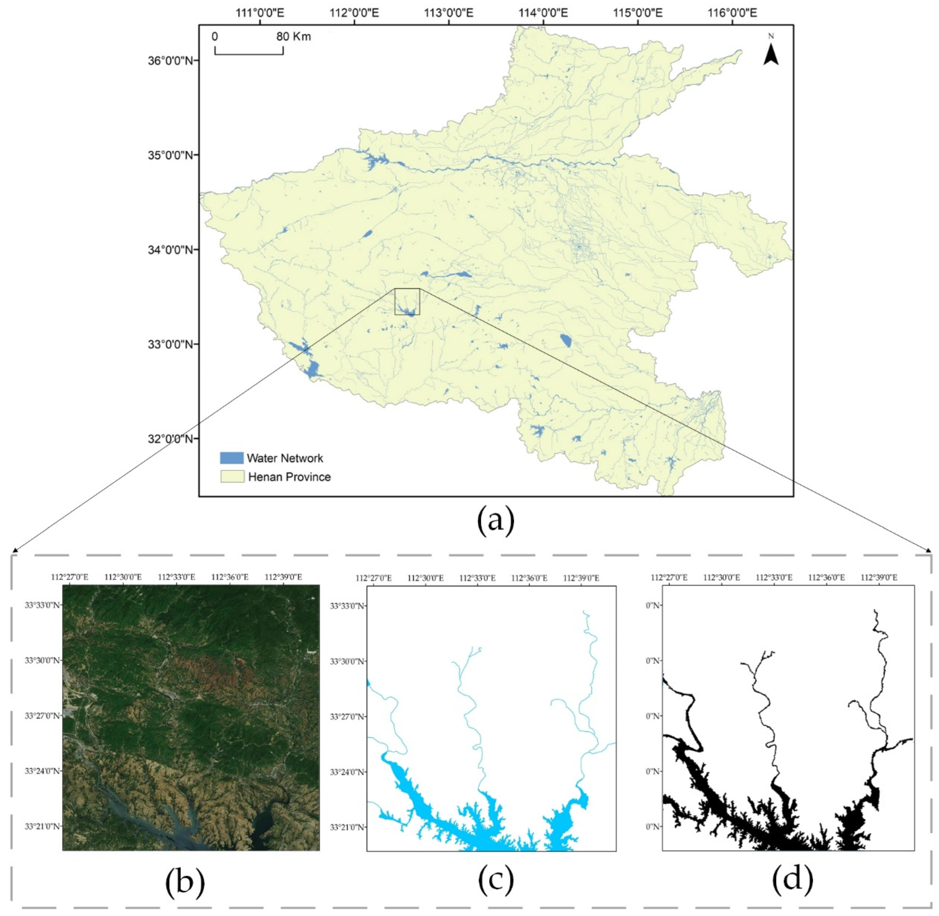
2.1. Study Area

As shown in Figure 1, Henan Province (110°21′E–116°39′E, 31°23′N–36°22′N) is located in the center of China, which has an area of 167,000 km2. Henan Province is the only one that spans the Yangtze River Basin, the Yellow River Basin, the Huaihe River Basin, and the Haihe River Basin, with numerous tributaries crisscrossing the territory. However, the total amount of water resources is at the middle level of the whole country, and the per capita water resources are less than 1/6 of the whole country. Meanwhile, there has been a serious shortage and uneven distribution in space and annual water due to the influence of latitude and climatic conditions. Therefore, high precision monitoring of the complete water stream in the study area is of great practical significance for the planning and utilization of water resources.

2.2. Data and Pre-Processing

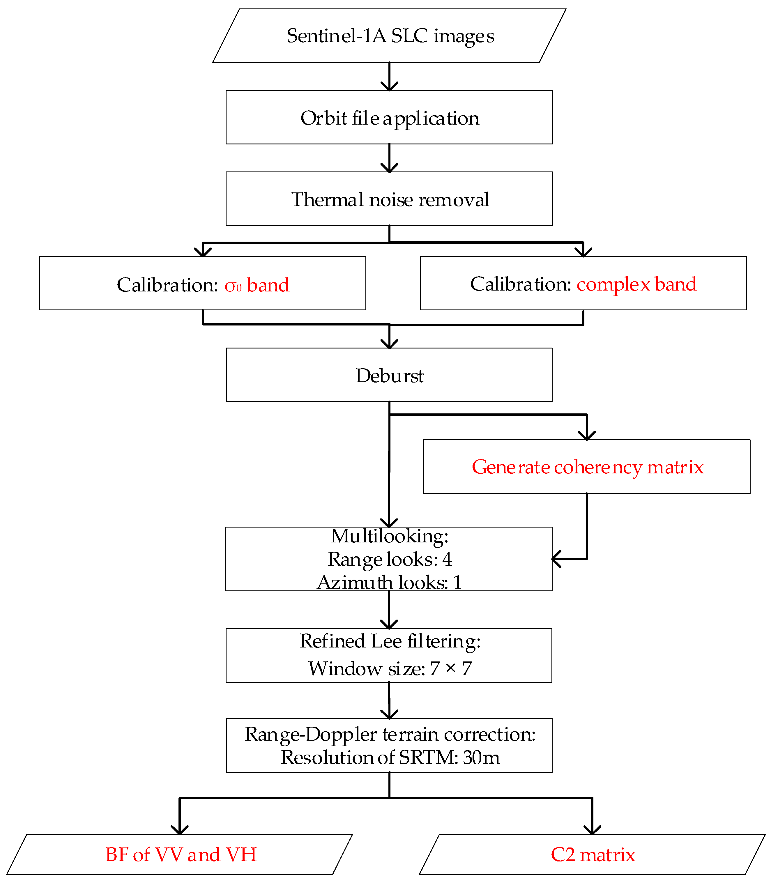
2.2.1. Sentinel-1A Data and Pre-Processing

Sentinel-1A SAR images acquired by the European Space Agency (ESA) have a short revisiting period of 12 days and a high spatial resolution of 5 × 20 m [46]. The parameters of the data are shown in Table 1. Single Look Complex (SLC) image, which includes amplitude and phase information, was chosen because it can provide abundant polarimetric information. As the scale of Sentinel-1A images can not cover the whole study area, a total of 14 scene SAR images from 14 May 2021 to 27 July 2021 were selected which can observe the entire study area. Among them, 13 scene SAR images were selected for model training and 1 scene SAR images for validation. Finally, 14 scene SAR images were spliced to obtain the result of water stream extraction in Henan Province.
The pre-processing steps for obtaining the BF and the polarimetric matrix from Sentinel-1A images were shown in Figure 2. For the same steps, the orbit file application, thermal noise removal, deburst, multi-looking, refined Lee filtering, and range-Doppler terrain correction were used. It should be noted that the number of range looks and azimuth looks is 4 and 1 in the step of multi-looking. In addition, the type of filter is refined Lee and window size is 7 × 7 pixels. Additionally, in the range-Doppler terrain correction, the shuttle radar topography mission (SRTM) with a resolution of 30 m was used to acquire the precise geographic information. Each burst was merged which has the effective signal parts by the operation of deburst. The impact of coherent speckle noise can be reduced by the multi-looking and filtering operation. Among the steps, the difference lied in that the output of calibration was σ0 band to obtain the BF, while the output of calibration was a complex band to obtain the polarimetric matrix. In addition, the coherency matrix was generated after the deburst to obtain the polarimetric matrix.

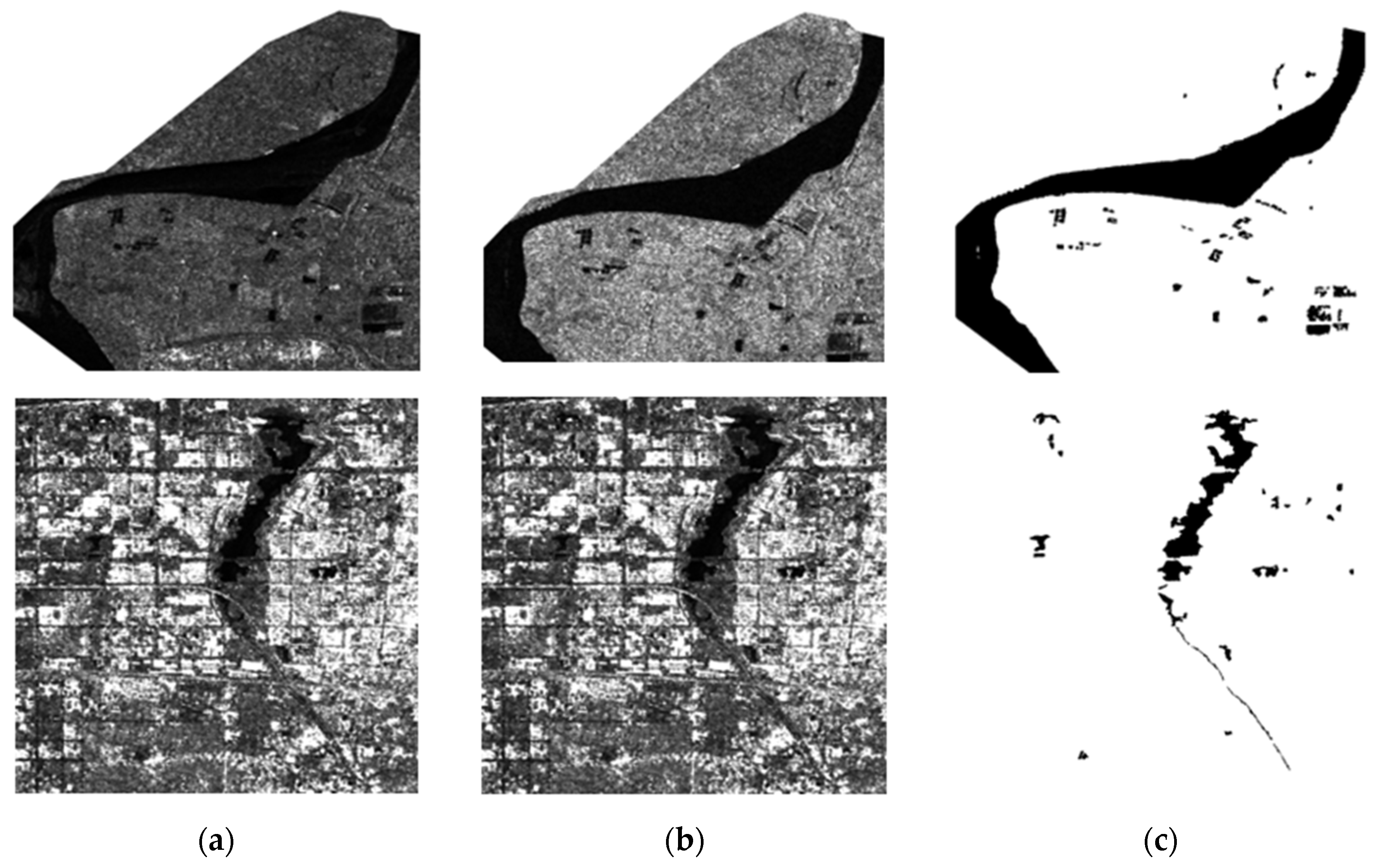
2.2.2. Ground Truth Data and Pre-Processing

In order to obtain a comprehensive and accurate view of the water bodies, the labeling process of samples can be divided into three steps. The first step was using the traditional threshold method for preliminary mapping. In the second step, the preliminary mapping of water bodies was corrected by visual interpretation to obtain more accurate labeling. Images of the same area and similar dates obtained by Google Earth were used as references. By comparison, the mistakenly extracted road and hill shade could be removed. Finally, the binary map was created by setting the pixel values of water and non-water to 0 and 1, respectively.
The sample set was divided into 1024 × 1024 with a 50% overlap area to make the sample representative and the model stable. In the training process, a total of 1521 sliced pictures were obtained by the 13 scene SAR images. 80% of the sliced pictures were randomly selected as training sets and 20% as test sets. Eventually, 1217 pictures were used as training samples and 304 pictures were used as test samples. By obtaining the binary map of water or non-water, the parameters of the samples were illustrated in Table 2. Figure 3 shows the BF of VV and VH polarization and corresponding samples of two regions.

2.3. Water Stream Extraction

The flow chart of the proposed method was presented in Figure 4. After the data pre-processing, the water stream extraction method was mainly divided into 3 steps. In step 1, standard BFs were extracted and the PFs were obtained based on the model-based decomposition of dual-pol SAR data [47]. Additionally, the above features were used to form five groups of candidate feature combinations. In step 2, FFEDN was proposed based on U-Net, including feature-fused block, encoder, pyramid pooling module, and decoder in order to improve the ability to mine and fuse both BFs and PFs, thus, better representing the characteristics of water bodies. In step 3, the extraction results of the water stream with different combinations were explored based on FFEDN by quantitative and qualitative evaluation. Through the analysis of precision and efficiency, the optimal combination was selected.

2.3.1. Feature Acquisition and Combination
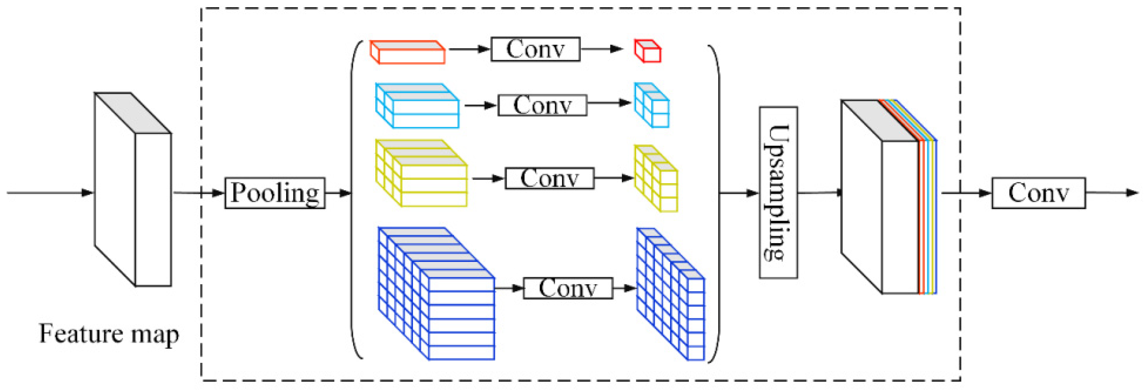
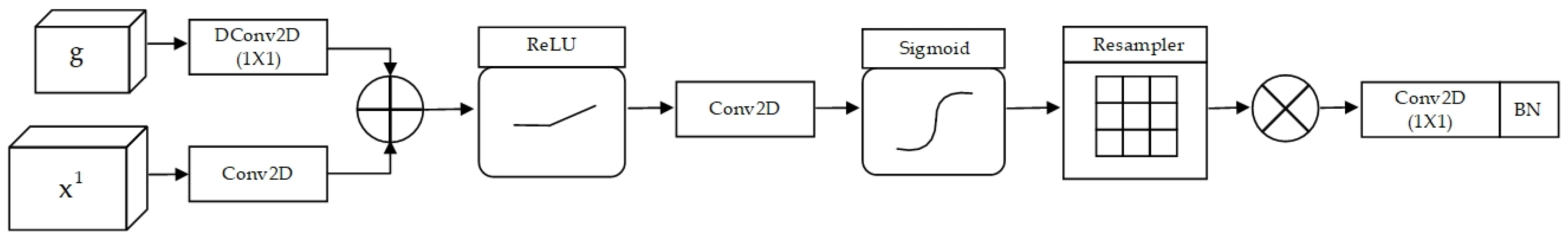
The BFs of Sentinel-1 with two polarization modes, namely VV and VH, can be obtained through the pre-processing. The BFs can be calculated as follows:
σ 0 V V = 10 l o g 10 D N V V A V V
σ 0 V H = 10 l o g 10 D N V H A V H
where D N is the original value of SAR image and A depends on the lookup table of auxiliary data.
The Sentinel-1 datasets used in this study were dual-polarimetric images with V V and V H polarization, for which the scattering matrix is defined as:
S = 0 0 S V H S V V
The corresponding target scattering vector k can be expressed as:
k = 2 S V H , S V V T
The Sentinel-1 dual-polarimetric SAR data can be represented by the following polarimetric covariance matrix:
C 2 X 2 = k k γ = c 11 c 12 c 21 c 22 = 2 S V H 2 2 S V H S V V 2 S V V S V H S V V 2
where γ represents the conjugate transpose and is the conjugate operator.
To make full use of the polarimetric information of Sentinel-1 images in water stream extraction, the polarimetric decomposition parameters (volume scattering m v , remaining scattering m s , and the difference between them m r a t ) were obtained from Sentinel-1 images by adopting the newly model-based decomposition adapted for dual-polarimetric SAR images [46].
Transforming C 2 X 2 into Stokes vector:
S _ = s 1 s 2 s 3 s 4 = c 11 + c 22 c 11 c 22 2 R e c 12 2 I m c 12
where R e c 12 and I m c 12 represent the real part and the imaginary part of c 12 , respectively.
Then, transforming S _ into the sum of three polarimetric components:
S _ = m v s _ v + m s s _ p + n s _ n
where s _ v represents an arbitrary volume model, s _ p represents the polarized Stokes vectors, n is noise term, s _ n is a randomly polarized Stokes vector that can be ignored using noise subtraction techniques [48], m v is the volume scattering component, and m s is the remaining scattering component.
Therefore, two items should be considered as follows:
S _ = m v 1 ± 0.5 0 0 + m s 1 c o s 2 α s i n 2 α c o s δ s i n 2 α s i n δ
α = 1 2 c o s 1 s 2 s 1 δ = arg s 3 + i s 4
where α and δ are the ratio parameters, symbol + is for H transmit, and − for V.
According to the above formulas, m v and m s can be calculated as follows.
m v = ± 2 R e c 12 arcsin c o s 1 c 11 c 22 c 11 + c 22 arccos arg 2 R e c 12 + 2 I m c 12
m s = c 11 + c 22 m v
The m r a t can be calculated as follows:
m r a t = m v m s
Subsequently, the three extracted PFs were obtained by decomposition.
After BF and PF were obtained by pre-processing, five combinations shown in Table 3 were formed for the extraction of the water stream. In previous studies, water extraction was based on BF. In order to effectively verify the performance of the model after adding PF, combination A was BFs. Different PFs, which represent different characteristics of the water body, were added to form different combinations.

2.3.2. FEEDN Model

FFEDN was built to obtain a more accurate result of the water stream by fusing and using the BFs and PFs. The structure of FFEDN, shown in Figure 5, consisted of four main components: feature-fused block, encoder block, pyramid pooling module, and decoder block. Feature fusion [49] and the encoder–decoder framework [50,51,52,53] were widely used in deep learning, which had proved to be effective for feature mining and fusing with different images and resolutions. The encoder–decoder framework was adapted as the backbone network and the skip connection was used between the encoder and decoder to obtain features with different resolution scales. The pyramid pooling module lay between the encoder and decoder part. The attention block is mainly inspired by the attention gate model [54], which is used to identify the irrelevant part of the model and learn the characteristics related to the task. The FFEDN attempted to mine water features of BFs and PFs and combine them together effectively, and the features of different scales were fused through encoder–decoder to improve the ability to extract the water stream.
In the feature-fused block, convolutional filters were set up to further mine the deep and correlation information from BFs and PFs. After the convolution layer, the batch normalization (BN) layers and ReLU activation function followed, respectively, which can improve network generalization capabilities and effectively avoid the problems of gradient explosion and gradient disappearance [55]. The fused feature maps were fed into the encoder and compressed into a potential space representation.
As shown in Figure 6, the pyramid pooling module (PPM) [56,57] fuses features of four different scales (1 × 1, 2 × 2, 3 × 3, and 6 × 6). The outputs of different levels contain the feature maps with different sizes. To maintain the weight of the global feature, the 1 × 1 convolution after each pyramid level was used to reduce the dimensions to 1 / N of the original features, where N is the size of the pyramid level. Then, the bilinear interpolation upsampling was used to restore the channel dimension of the low-dimensional feature map to the original feature map. Finally, different levels of features were concatenated as the final global feature of pyramid pooling. The pyramid pooling module collected multi-level features of multi-scale water bodies, such as lakes or small rivers with different characteristics, and combined them with the original feature map extracted for the encoder.
Then, the decoder aimed to reconstruct the spatial representation, which mapped the feature vectors back to the original input image size. The skip connection between the encoder and decoder is developed to provide rich fundamental information. At last, a water–non-water binary map was generated by convolution operation with the kernel size of 1 × 1. Especially, as shown in Figure 7, the attention block (ABL) [58,59] was used in the decoder to make the network focus on water stream extraction by identifying the irrelevant part and learning the characteristics related to the task. The g represents the gating signal output from the downsampling layer and X 1 represents the feature map of the upsampling layer passed by the skip connection. DConv2d represents the mean pool after using the dilated convolution kernel. Then, the gate signal and feature map are connected and the ReLU activation function, dimension reduction, and Sigmod activation are used. The results are the dot multiplied with X 1 to obtain the features concerned.
It should be noted that the proportions of water and background pixels were imbalanced, thus, using Dice loss which was designed to address the extremely imbalanced samples [60] to solve the problem. In the task of water bodies extraction, the Dice loss function was as follows:
L D i c e = 1 D i c e
where L D i c e represents the Dice loss and D i c e represents Dice coefficient. Using L D i c e   ϵ   0 ,   1 to balance the importance of water and non-water pixels which can avoid non-water pixels dominating the gradient. Larger D i c e puts more weight on water pixels.
The calculation equation of the Dice coefficient was as follows:
D i c e = 2 A B A + B
where A B specifies the intersection of the generated results and the ground truth value and A and B represent the pixel number of the extraction results and ground truth, respectively. The extraction performance was better when the Dice coefficient was higher.
In summary, the FFEDN model contained four blocks: feature-fused block, encoder block, pyramid pooling module, and decoder block. The feature-fused block was used to extract and fuse the water features from different kinds of features. The encoder block, which extracts features using convolution, increased the receptive field by the pool layer. The pyramid pooling module could realize multi-scale feature extraction from the feature map of both small rivers or large water bodies with different characteristics. In the decoder, through deconvolution and the attention block, the features were reproduced, and the upsampling was restored to the original size of the input. The process used supervised learning to discover internal correlations between the BF and PF and extract as much useful information as possible. The detailed parameters of FFEDN are shown in Table 4.

2.3.3. Optimal Combination Selection

In order to select the optimal combination, confusion matrix was used to evaluate the extraction results. As shown in Table 5, the definitions of the four indicators were given in the confusion matrix.
Precision, recall, intersection over union (IoU), overall accuracy (OA), and average accuracy (AA) were chosen as evaluation indicators to carry out quantitative analysis. The calculations of them were illustrated in the Equations (15)–(19), respectively. High precision means that the extraction results are more accurate. A high value of recall means that the model can find more water bodies in the image. IoU represents the overlap ratio of the model extraction results.
Precision:
Precision = TP TP + FP
Recall:
Recall = TP TP + FN
IoU:
IoU = TP TP + FP + FN
OA:
OA = TP + TN TP + FN + FP + TN
AA:
AA = 1 2 TP TP + FN + TN FP + TN
The McNemar test [61] was used to access the statistical significance of differences in the extraction accuracy. McNemar’s test principle is based on the evaluation of a contingency table with a 2 × 2 dimension considering only correct and incorrect points for two different methods. (Table 6).
In the relative comparison between different combinations in our manuscript, the chi-square ( χ 2 ) has one degree of freedom and uses exclusively discordant samples as shown in Equation (20):
χ 2 = ( f 12 f 21 ) 2 f 12 + f 21

3. Results

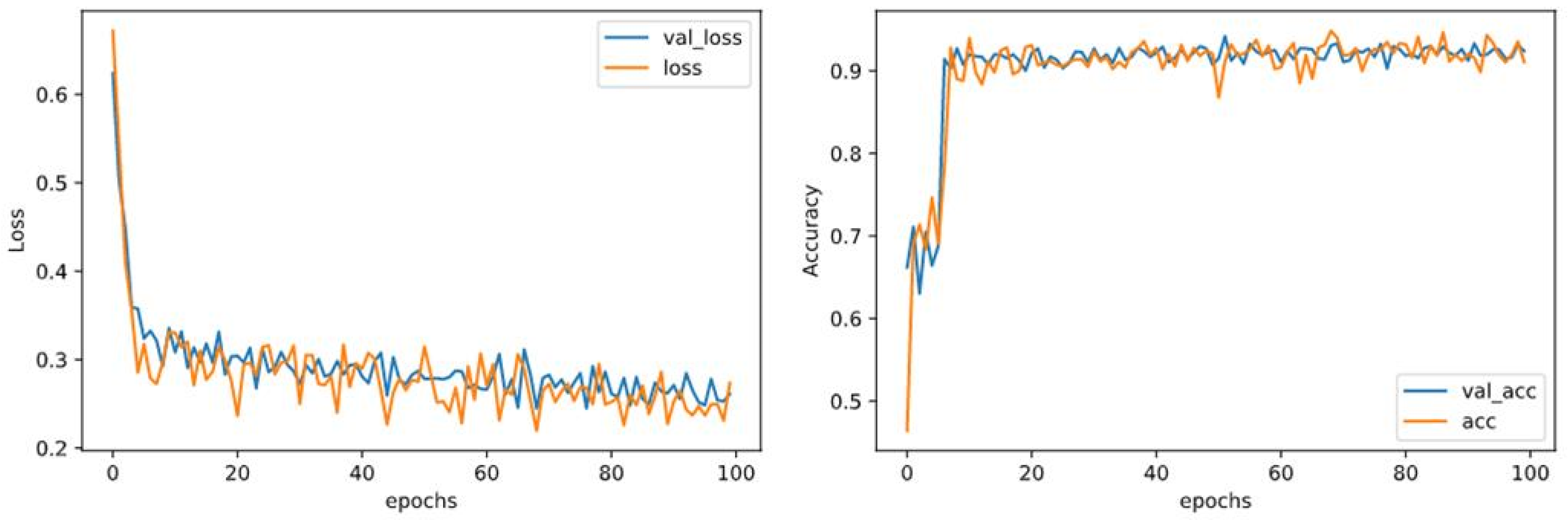
3.1. Implementation Details

All of the experiments were completed in the TensorFlow environment with GeForce RTX 3080Ti and 64G RAM. The FFEDN was trained by an Adam optimizer [57,58] which has computational efficiency and low memory requirements. The weight decay was set to 0.004 and the learning rate was set to 0.0001. The model was trained on 100 epochs to obtain the final results and the batch size was 32. The hardware and software configuration of the network was presented in Table 7.
The FLOPs of FFEDN were 62,049,671 and the model size was 359 MB. On average, it took around 4–5 h to train the model. To ensure a fair comparison, all parameters were set as the same in all experiments. Figure 8 showed the loss and accuracy plot for FFEDN obtained on training and validation images of the SAR sub-image dataset.

3.2. Evaluation of Different Combinations with FFEDN

There were 14 images in the experiment, 13 of which were used to train the FFEDN model. After training the model, the remaining SAR image not included in the training process was used for validation. In the task of water stream extraction, the fine water bodies were easily omitting, the shadows were lightly classified as water bodies, and the small rivers were easily extracted incompletely. All the above phenomena will lead to inaccurate results of water stream. Thus, three different areas were selected, namely, rural (Region A), hilly (Region B), and urban (Region C) which includes water bodies with different characteristics, as shown in Figure 9a–c, respectively. The selected area was 1024 × 1024, as shown in the orange rectangle in Figure 9. The relatively complete water stream can be constructed if the water bodies can be extracted in the different areas.

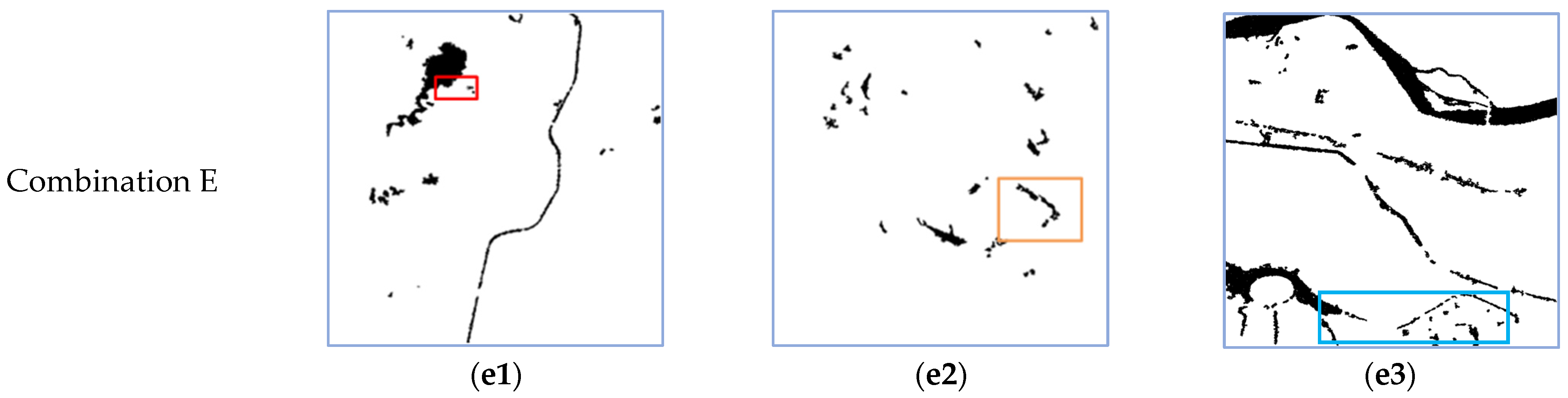
3.2.1. Qualitative Evaluation

The five combinations shown in Table 3 were used as the inputs of FFEDN and the optimal one was explored through qualitative evaluation and quantitative evaluation, respectively. The extraction results of Region A, B, and C using different combinations were shown in Figure 10.
Whether in Region A, B or C, when the Combination C was used as input, the extracted results were more refined and complete. In Region A, as shown in Figure 9c, both the large water bodies and fine water bodies were extracted more completely and accurately. In Region B, as shown in Figure 10(c2), especially in the orange rectangle, the erroneous extraction of hilly shadows as water was effectively reduced. In Region C, marked with blue rectangle in Figure 10(c3), the small rivers flowing through the urban area could be effectively extracted.
For Combination A, there were errors of false and missing information in extracting fine water bodies, as shown in Figure 10(a1). The shadow of hills was extracted mistakenly as a water body in the Region B marked with a yellow rectangle, as shown in Figure 10(a2). The river in Region C was not extracted connectively, as shown in the blue rectangle in Figure 10(a3). For Combination B, the fine water stream is extracted accurately to a certain degree compared with Combination A, as shown in Figure 10(b1). However, the shadows were still mistakenly classified as a water body in Figure 10(b2). The results of river extraction in the Region C were more accurate which also had a missing extraction in the blue rectangle in Figure 10(b3). For Combination D, the extraction result in Figure 10(d1) was complete. However, the hilly shadow was still wrongly classified as a water body in Figure 10(d2) and the river flowing through the Region C in Figure 10(d3) was not correctly identified to some extent. For Combination E, the fine water body, hilly shadows, and small rivers were not correctly extracted.

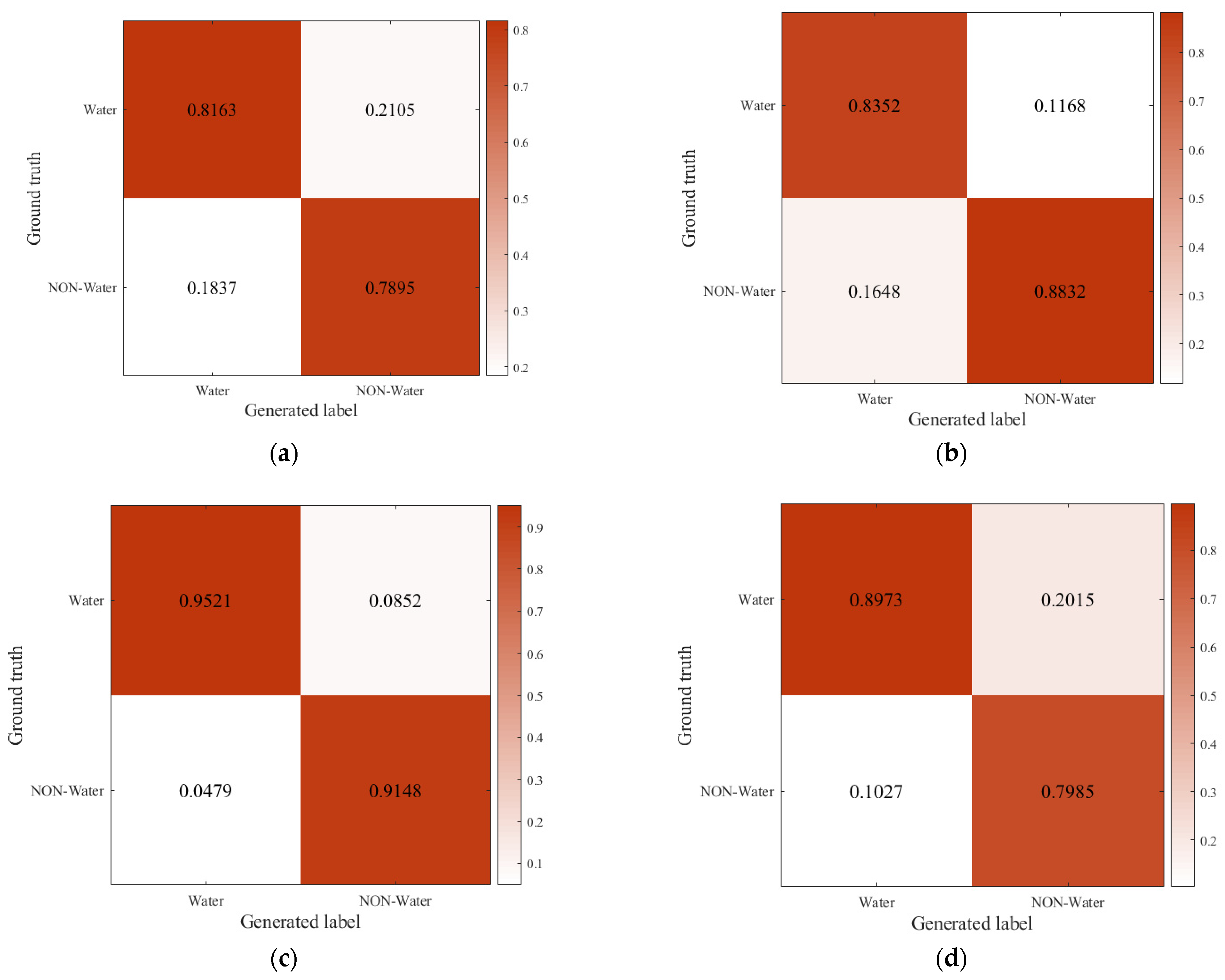
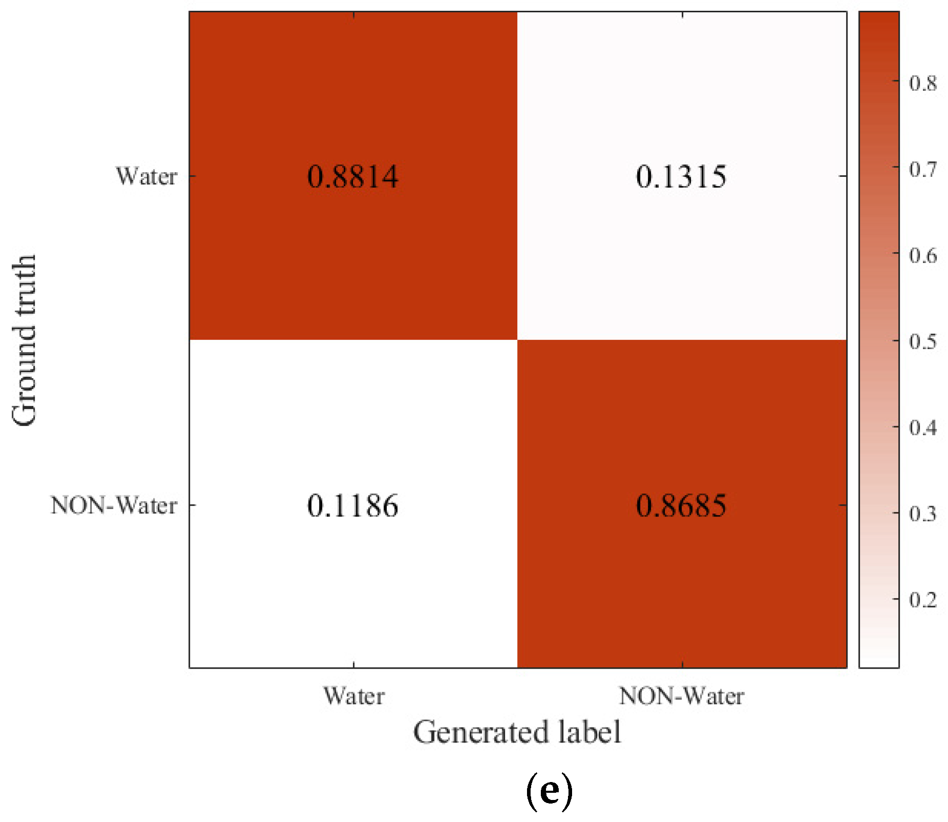
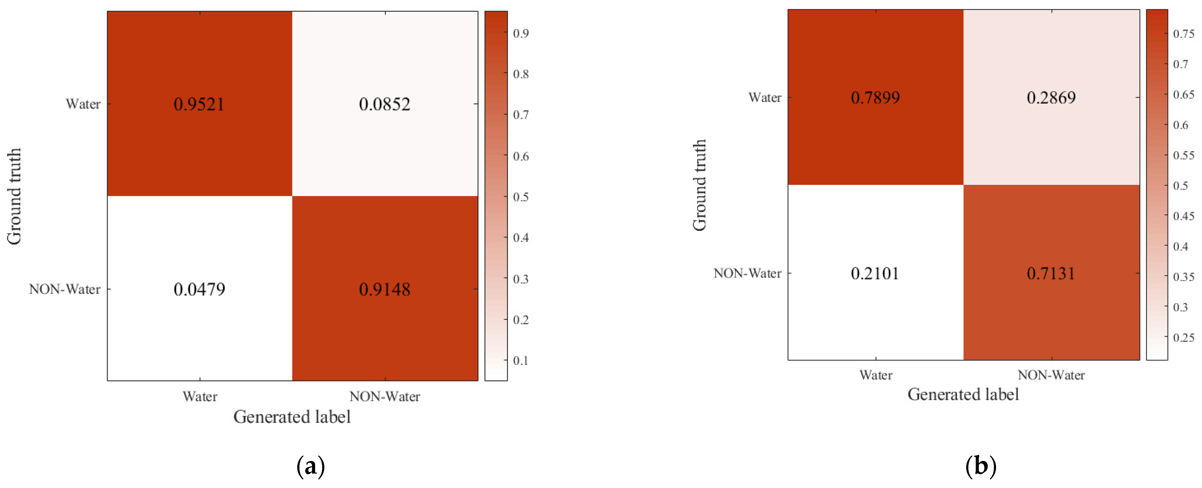
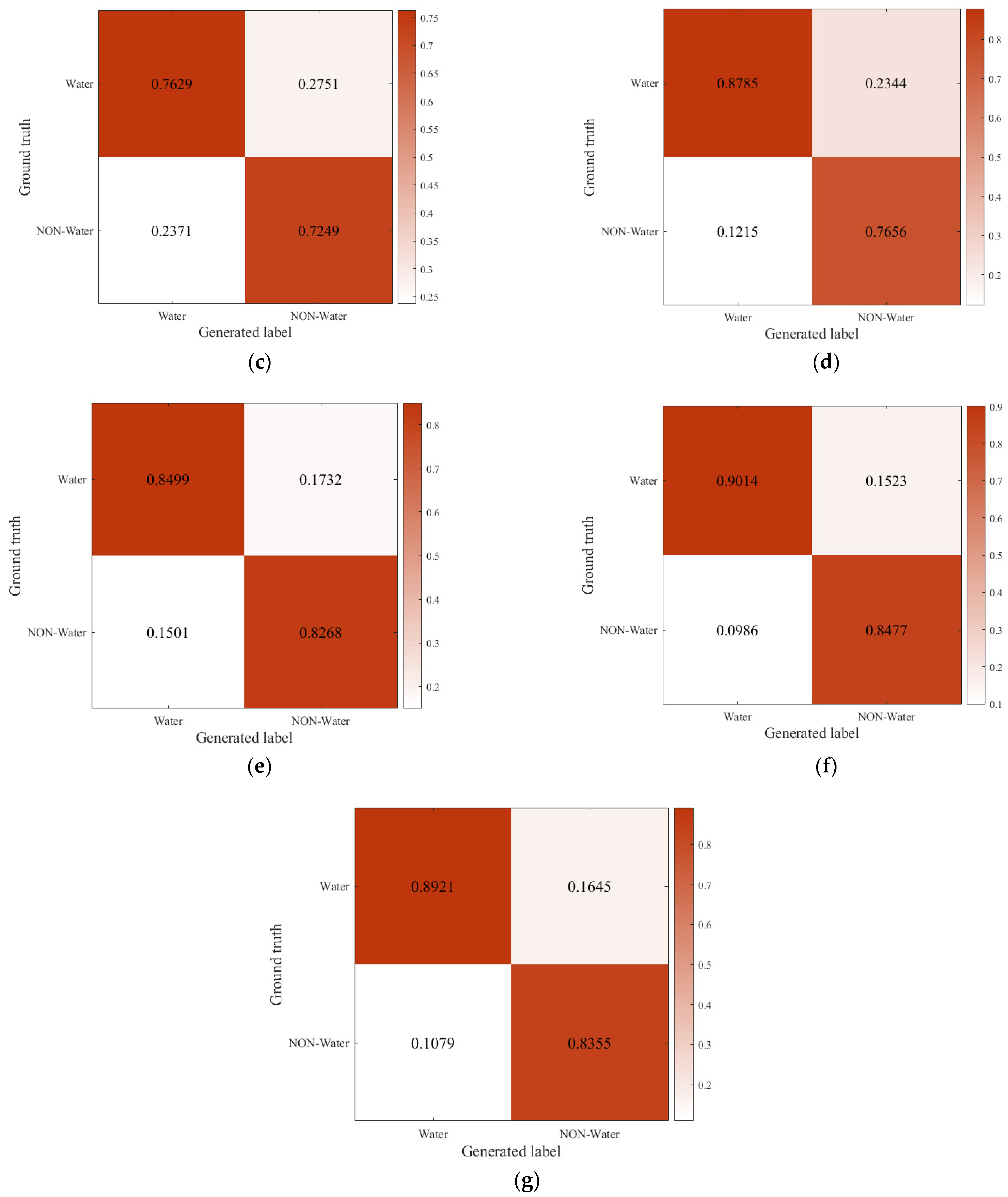
3.2.2. Quantitative Evaluation

The validation samples were fed into the FFEDN, then the outputs of models were compared with the labels to generate confusion matrices, which were shown in Figure 11. According to the confusion matrices, the different combinations were quantitatively evaluated.
The results were listed in Table 8. Among them, the indicator values were lowest when using Combination A as input. The precision, recall, OA, and AA were around 80% and the IoU was lower than 70%. Combination C achieved the best accuracy which precision scored 95.21%, recall scored 91.79%, IoU scored 87.73%, OA scored 93.35%, and AA scored 93.41%. This was because the scattering type of water body in the SAR image is surface scattering which can be represented by m s . Therefore, the indicator value was highest when using Combination C as input. Precision of Combination B was 83.52% because m v is different from the characteristics of water body in the SAR image. Precision, recall, IoU, OA, and AA of Combination D were lower than Combination C 5.48%, 10.13%, 7.96%, 13.05%, 8.56%, and 8.82%, respectively. This was because the features of m v and m r a t have a negative influence on water extraction, resulting in low indicator values. Precision, recall, OA, and AA of Combination E were all above 85%, but the IoU was still low which was due to the negative effects of m v and m r a t .
McNemar test results highlight that the extraction results between different Combinations. The chi-square value between Combination A and other Combinations (B, C, and D) were given in Table 9. The χ 2 values were larger than 3.84 and the results confirm the better performance after fusing BFs and PFs.

3.3. Ablation Study of FFEDN with Feature Combination C

In order to verify each improvement measures’ effectiveness in FFEDN, the experiments were conducted. The ablation study contains two parts: pyramid pooling module and attention block. The baseline was FFEDN with the feature Combination C as input. Table 10 showed different strategies for the ablation study.

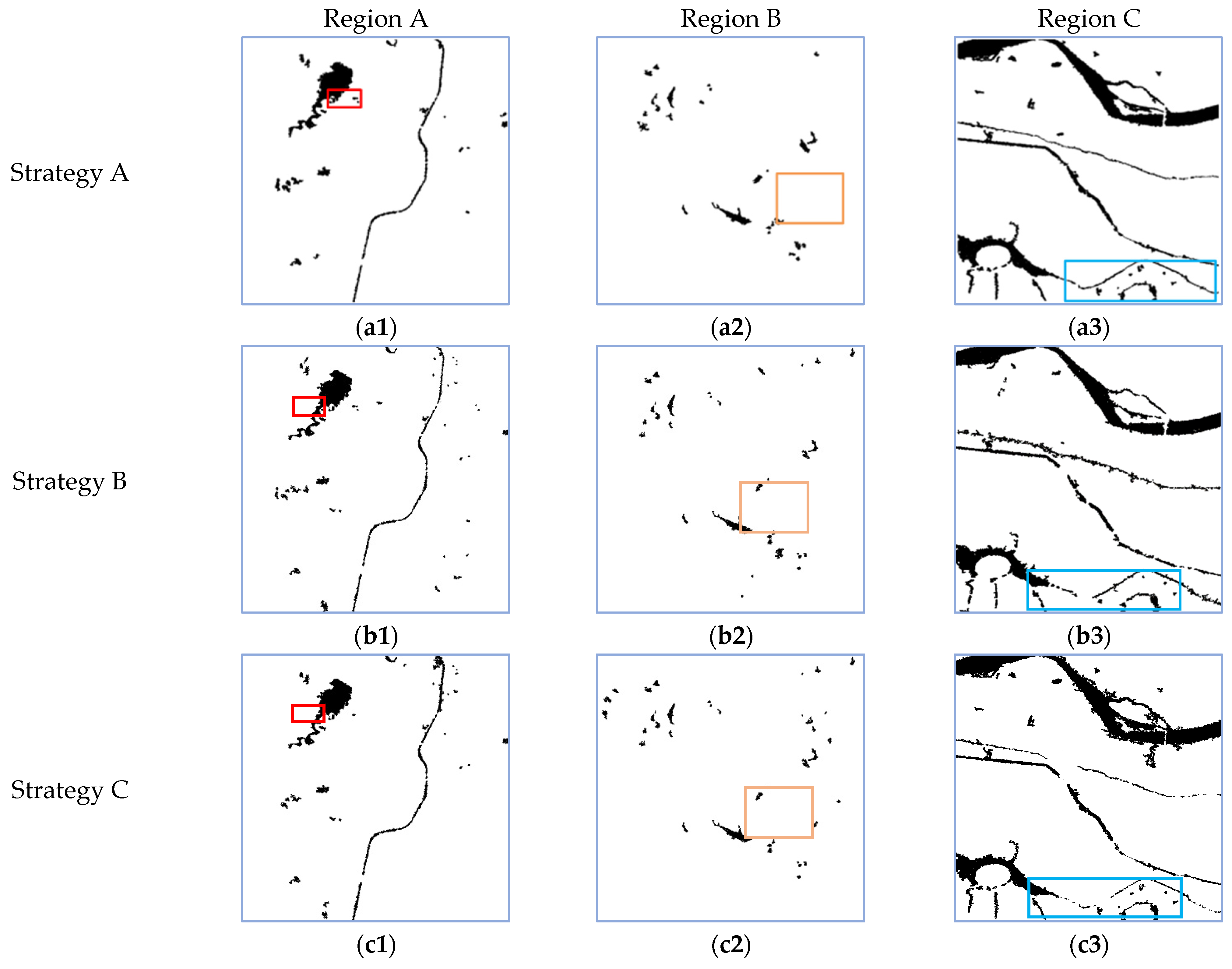
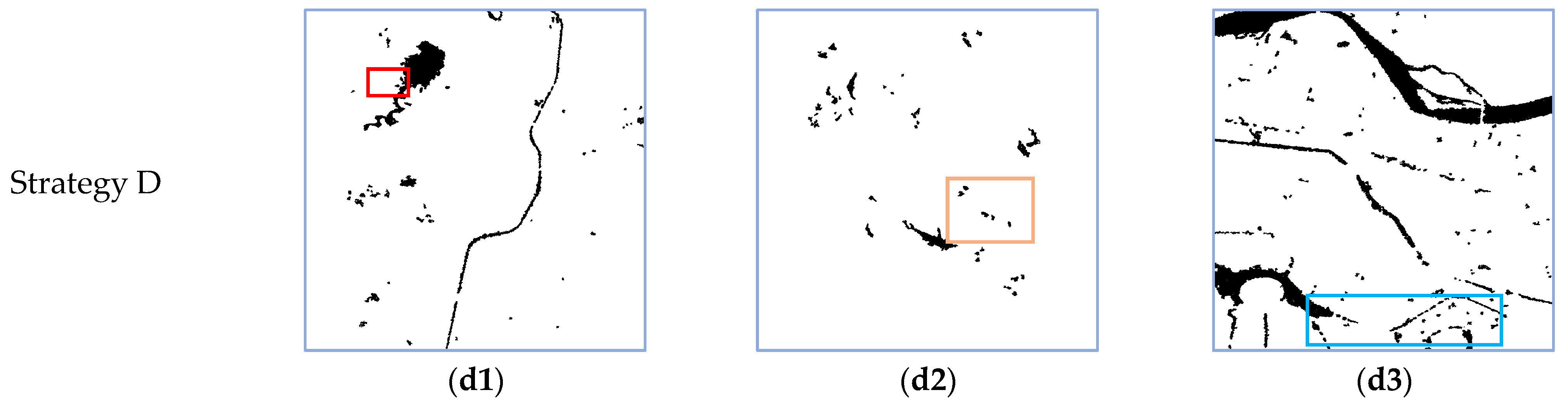
3.3.1. Qualitative Evaluation

The extraction results of the different strategies were shown in Figure 12. After removing the PPM from FFEDN, the details such as small rivers tributaries in the middle of the rivers were missed, as shown in Figure 12(b3). When ABL was removed, the extraction result in Region B was not accurate with classifying shadows as water bodies, as shown in Figure 12(c2). When both PPM and ABL were removed, the model only can produce low confidence predictions and blurred boundary.

3.3.2. Quantitative Evaluation

As can be seen from Table 11, after removing the PPM, the precision, recall, IoU, OA, and AA of the water extraction task were decreased by 6.04%, 6.25%, 12.72%, 8.15%, and 11.49%, respectively. After removing the ABL, the indicators were decreased as well. When the model was trained without PPM and ABL, the indicators were lowest. Both PPM and ABL improved the performance of FFEDN.

3.4. Evaluation of Different Methods with Feature Combination C

3.4.1. Compared Methods

In order to verify the effectiveness of the methods proposed, several machine learning methods and deep learning methods were selected for comparison. The classical machine learning methods (RF, SVM) and some CNN-based methods (U-Net, U-Net-Resnet [62], MSF-MLSAN [41] and WENET [42]) were selected. SVM is a supervised classification method for binary cases. It uses a subset of training samples (called support vectors) close to the decision boundary to calculate the linear decision hyperplane. RF is a classifier that consists of many decision and regression trees to train and predict the classification results. The U-Net and U-Net-Resnet model were widely used for feature extraction and water extraction. MSF-MLSAN [41] was proposed to extract water bodies in mountain regions by using millimeter wave SAR images and had achieved potential performance. WENET [42] integrates the features of SAR images at different scales for water extraction. The hyperparameters of the SVM and RF were listed in Table 12.

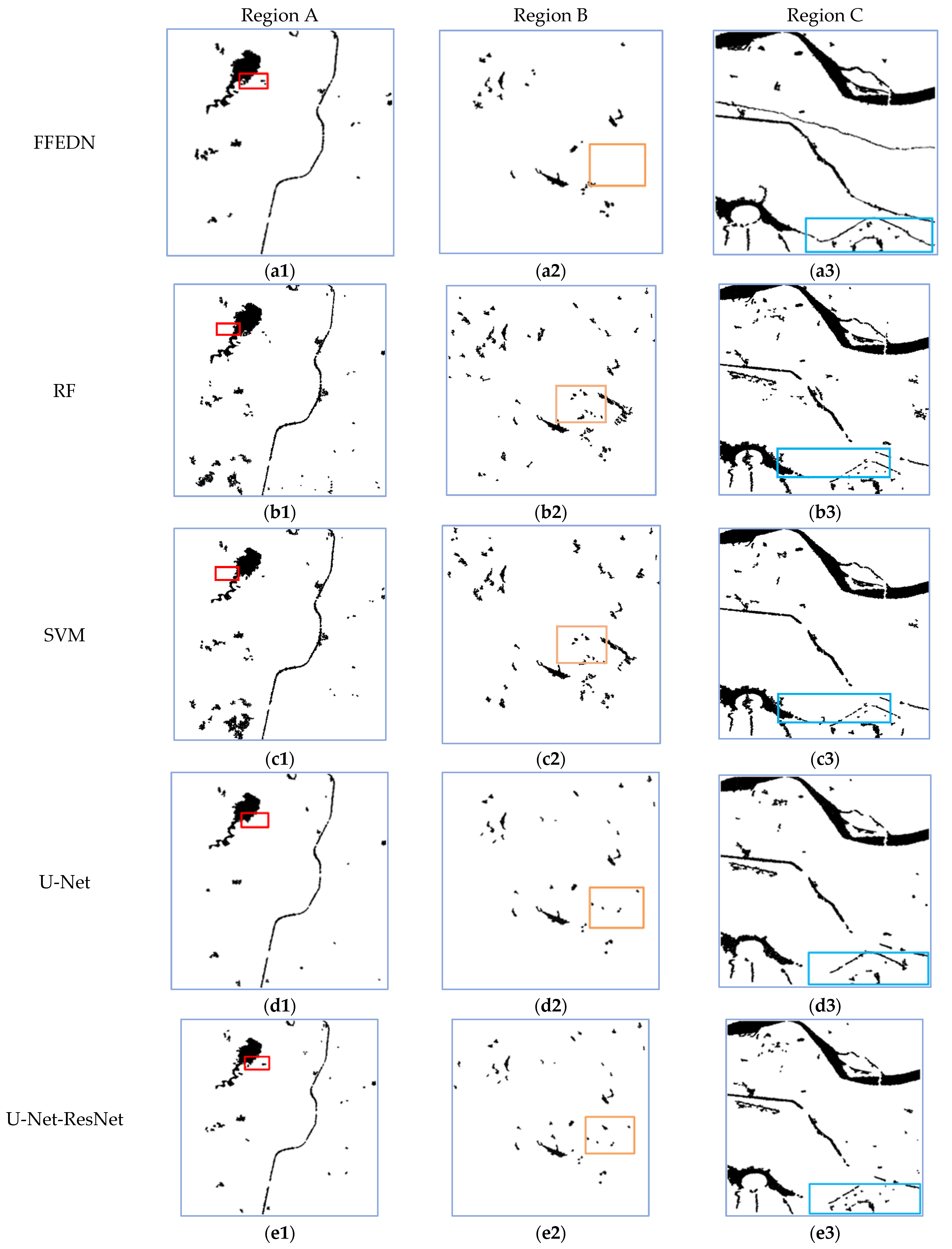
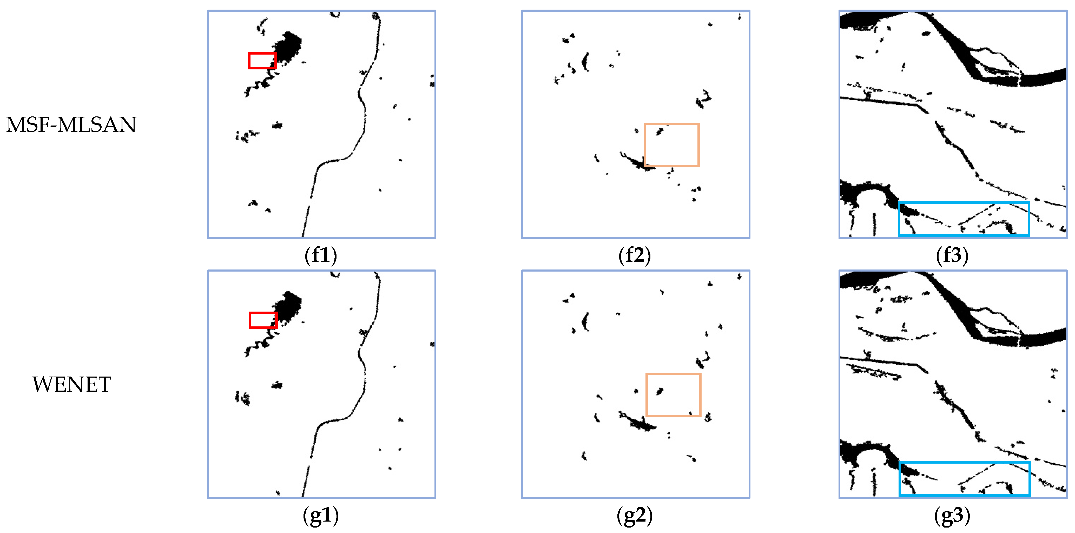
3.4.2. Qualitative Evaluation

The extraction results of the seven methods selected above were shown in Figure 13. All methods extracted water accurately in a large area and the proposed method had the best effect, especially mapping the water bodies in Region B and drawing small rivers flowing through the Region C thoroughly, as shown in Figure 13(a2,a3). For machine learning methods, as shown in Figure 13(b1,c1), RF and SVM can also extract small water bodies. However, the two methods mistakenly extracted hilly shadows as water, as shown in Figure 13(b2,c2). Meanwhile, as shown in Figure 13(b3,c3), the results presented a missing extraction phenomenon of relatively small rivers as shown in the blue rectangle. For deep learning methods, the water body in Region A was extracted accurately as shown in Figure 13(d1–g1). As shown in Figure 13(f2,g2), MSF-MLSAN and WENET mapped the water body in Region B accurately without extracting shade mistakenly. Meanwhile, the other deep learning methods also extracted hill shade mistakenly. As shown in Figure 13(d3–g3), the four deep learning methods presented a missing extraction phenomenon of relatively small rivers as shown in the blue rectangle, which was due to the influence of urban buildings or trees.

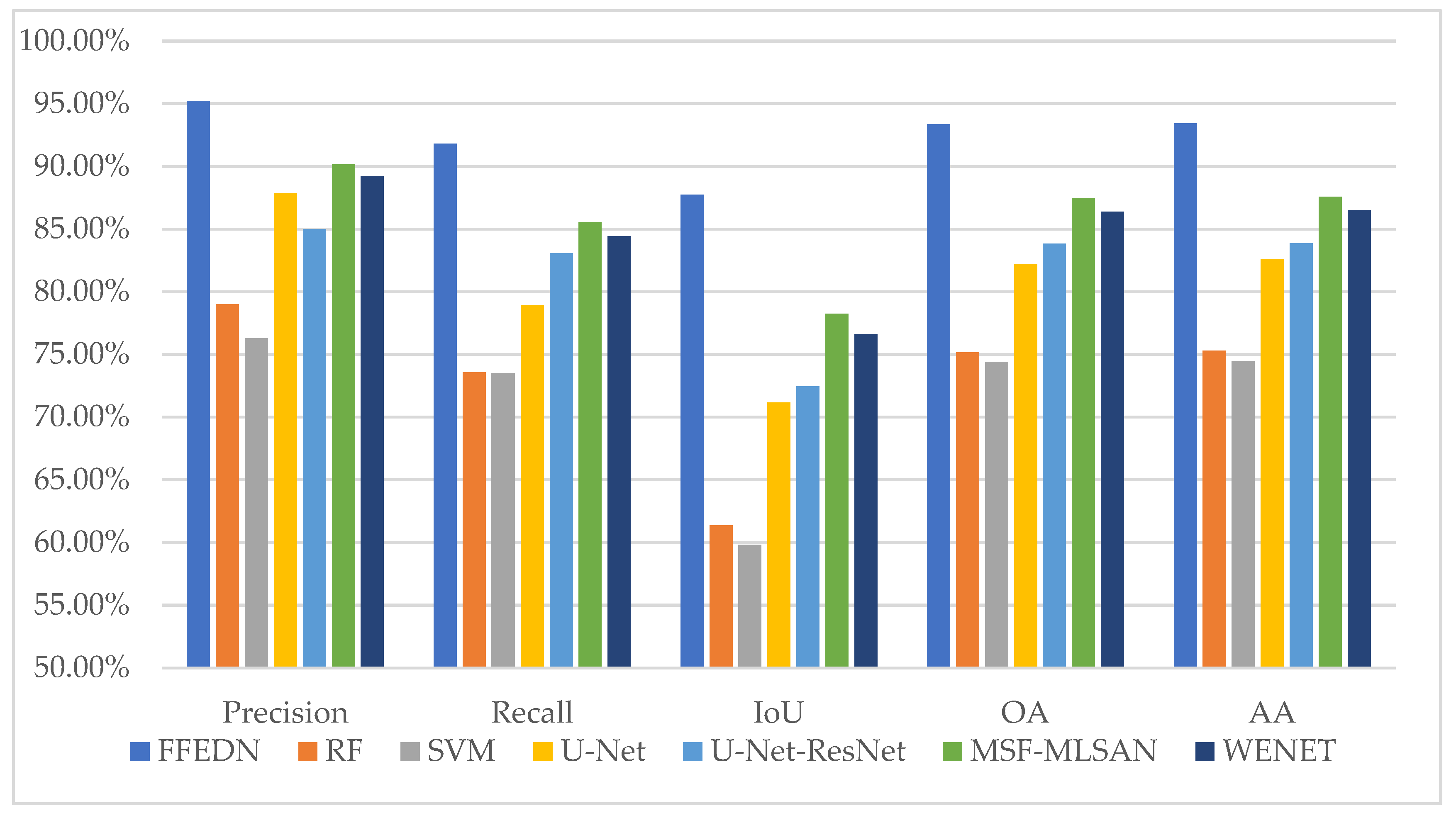
3.4.3. Quantitative Evaluation

The validation images were fed into the models, then the outputs of models were compared with the labels to generate confusion matrices, which are shown in Figure 14. According to the confusion matrices, the methods were quantitatively evaluated. The results were listed in Table 13.
Among them, the proposed FFEDN achieved the best accuracy. Precision scored 95.21%, recall scored 91.79%, IoU scored 87.73%, OA scored 93.35%, and AA scored 93.41%. The machine learning methods cannot effectively establish a mapping relationship to classify each pixel, so values of indicators were lowest. Especially in the Region B and Region C, complex scenarios made them more difficult to extract water accurately. For deep learning methods, the indicator values improved compared with machine learning methods. The precision of U-Net and U-Net-ResNet was 87.85% and 84.99%, respectively, which indicates that the encoder–decoder network can fuse abstract high-level information and detailed low-level information. MSF-MLSAN and WENET performed well and the indicators were higher. However, compared with the proposed method, the other deep learning methods can not map a complete water stream because the water bodies in complex scenes were difficult to extract.
To objectively assess the model ability of each method, a visual comparison of the accuracy evaluation indicators precision, recall, IoU, OA, and AA were presented in Figure 15. The OA can be ranked in the following order: FFEDN > MSF-MLSAN > WENET > U-Net-ResNet > U-Net > RF > SVM. It demonstrated that the deep learning methods outperformed the machine learning methods on the task of water stream extraction. Furthermore, the proposed network model outperformed other models.

3.5. Extraction Result of Study Area

As shown in Figure 16, using the proposed model, FFEDN, the final water stream of the study area was extracted from the stitched image of the 14 SAR images. It can be shown that rivers, lakes, reservoirs, and ponds were all extracted. The regional distribution of water resources in Henan Province was uneven. The plain areas of eastern and northern Henan were densely populated, which were the main grain producing areas. However, the serious shortage of water resources in this area directly restricted the sustainable development of the local national economy. Accurate extraction of the water stream can provide powerful data for surface water resources management and planning as well as drought and flood disaster prevention, and it can also contribute to social and economic development and ecological protection. The Landsat-8 optical image on 18 May 2021 with cloud cover of 0.13% was used for qualitative evaluation. The band combinations of the Landsat-8 image can extract specific information to help better understand the ground objects. The image of bands B4 (Red), B3 (Green), and B2 (Blue) combination was defined as a pseudo-color image, as shown in Figure 16b. As shown in Figure 16b–d, compared with the optical image and the ground truth, the tributaries were extracted accurately, thus, constructing a more connective water stream. The code of the implemented methods is available at https://github.com/yuandadada/SARwater (accessed on 15 November 2022).

4. Discussion

In this work, the water stream extraction method using BF and PF was carried out. First, the BFs were extracted and PFs were obtained through model-based decomposition. Then, a new model FFEDN was developed for the water stream extraction task, which mined and combined water features from both BFs and PFs. Lastly, by comparing the results of the water stream extraction with different combinations, the optimal one was chosen. The results showed that the extraction results were improved indicating that PF can effectively manifest the physical scattering mechanism of water bodies in SAR images. To further verify the effectiveness of the proposed method, two machine learning methods and the other four deep learning methods were chosen to compare with FFEDN and the results demonstrated the validity of FFEDN in the extraction of the water stream. The water stream of the study area was extracted by the method proposed in this paper.
First of all, the model-based decomposition of dual-pol SAR data was used to extract the polarimetric features from Sentinel-1A SAR data. Other decomposition methods, such as Freeman and Yamaguchi, have been widely used in many applications. However, most of these methods were designed to be used with quad-pol data and always lead to the loss of polarimetric information when decomposing the dual-pol SAR data. Fortunately, the model-based decomposition used in this paper can extract important underlying physical information from Sentinel-1A images, providing the data for the correct interpretation of parameters of different polarimetric components.
Moreover, this paper demonstrated that the FFEDN outperformed the machine learning methods SVM and RF, and deep learning methods U-Net, etc. Based on the optimal feature, the most representative machine learning methods and deep learning methods, RF, SVM, U-Net, U-Net-Resnet, MSF-MLSAN, and WENET, were chosen for comparison. As can be seen in Figure 13, the two machine learning methods did not achieve good results in both simple and complex environments. The deep learning methods achieved good results in the water extraction when the scene was not complicated, but the extraction accuracy in the hilly area affected by shadows and buildings was lower, so these deep learning methods found it impossible to form a connected water stream. In addition, the comparative deep learning methods did not input the PFs when establishing the model. In particular, the proposed FFEDN showed good extraction performance in every scene, exceeding 95%, 91%, 87%, 93%, and 93% of precision, recall, IoU, OA, and AA, respectively.
However, the local rivers may have had seasonal cut offs at the time of data acquisition and the extracted water stream may not be accurate. This problem should be considered and overcome by using multi-temporal data in the same area. Meanwhile, because of the small shape and narrow width of lakes and rivers are similar to the spatial resolution of the SAR images. Another work direction is to apply the proposed method with higher resolution SAR data to extract the water stream more connectively.

5. Conclusions

In this study, a deep learning method was proposed for water stream extraction named FFEDN using Sentinel-1A SLC images. The method first obtained the BFs and the PFs from Sentinel-1A images using model-based decomposition. Then, based on U-Net, FFEDN was constructed. Next, BF and PF, which formed different combinations, were used as inputs to FFEDN to select the optimal features. Finally, through qualitative analysis, the accuracy, integrity, and connectivity of the extracted water body were analyzed and the optimal feature combination was selected. Through a comparison with two machine learning methods and four other deep learning methods, the application potential of the proposed method in water stream extraction was verified. The proposed method achieved the best results in both qualitative and quantitative analysis. Therefore, FFEDNN was used to extract the water stream of Henan Province and the results were analyzed accordingly.
Furthermore, a few interesting things were found in this paper. For example, the combination of BF and PF can obtain higher extraction accuracy.
This study demonstrated the significance of PFs from Sentinel-1 data. Meanwhile, deep learning methods had great potential for water stream extraction. In the future, with the continuous optimization of decomposition methods and deep learning models, water streams will be extracted more accurately.

Author Contributions

Conceptualization, D.Y., C.W. and L.W.; data curation, X.Y. and Z.G.; investigation, Z.G., X.D. and N.L.; methodology, D.Y., Z.G. and C.W.; supervision, Z.G. and N.L.; writing—original draft, D.Y. and L.W.; writing—review and editing, C.W., L.W., X.Y., J.Z. and N.L. Validation, J.Z. All authors have read and agreed to the published version of the manuscript.

Funding

This research was funded by Scientific and Technological Research and Development Program of Henan Province (222103810100), the Plan of Science and Technology of Henan Province (212102210101), the Key R&D Project of Science and Technology of Kaifeng City (22ZDYF006) and the Open Fund Project of Key Laboratory of Natural Resources Monitoring and Supervision in Southern Hilly Region, Ministry of Natural Resources of China (NRMSSHR2022Z01).

Data Availability Statement

The authors would like to thank the ESA for providing the research data at https://scihub.copernicus.eu/dhus/#/home (accessed on 15 November 2022).

Acknowledgments

The authors would like to thank the ESA for providing the sentinel-1A SAR data for water applications.

Conflicts of Interest

The authors declare no conflict of interest.

References

  1. Peng, G. Modern Water Network Construction Practice and Its Effectiveness Analysis of Linyi City; Shandong Agricultural University: Taian, China, 2012. [Google Scholar]
  2. Cheng, T.; Liu, R.-M.; Zhou, X. Water Information Extraction Method in Geographic National Conditions Investigation Based High Resolution Remote Sensing Images. Bull. Surv. Mapp. 2014, 4, 86–89. [Google Scholar]
  3. Dong, Y. River Network Structure and Evaluation of Its Characteristics; Tianjin University: Tianjin, China, 2018. [Google Scholar]
  4. Wan, L.; Liu, M.; Wang, F.; Zhang, T.; You, H.J. Automatic extraction of flood inundation areas from SAR images: A case study of Jilin, China during the 2017 flood disaster. Int. J. Remote Sens. 2019, 40, 5050–5077. [Google Scholar] [CrossRef]
  5. Feyisa, G.L.; Meilby, H.; Fensholt, R.; Proud, S.R. Automated Water Extraction Index: A new technique for surface water mapping using Landsat imagery. Remote Sens. Environ. 2014, 140, 23–35. [Google Scholar] [CrossRef]
  6. Ogilvie, A.; Belaud, G.; Delenne, C.; Bailly, J.-S.; Bader, J.-C.; Oleksiak, A.; Ferry, L.; Martin, D. Decadal monitoring of the Niger Inner Delta flood dynamics using MODIS optical data. J. Hydrol. 2015, 523, 368–383. [Google Scholar] [CrossRef] [Green Version]
  7. Isikdogan, F.; Bovik, A.; Passalacqua, P. RivaMap: An automated river analysis and mapping engine. Remote Sens. Environ. 2017, 202, 88–97. [Google Scholar] [CrossRef]
  8. Domeneghetti, A.; Tarpanelli, A.; Brocca, L.; Barbetta, S.; Moramarco, T.; Castellarin, A.; Brath, A. The use of remote sensing-derived water surface data for hydraulic model calibration. Remote Sens. Environ. 2014, 149, 130–141. [Google Scholar] [CrossRef]
  9. Vimal, S.; Kumar, D.N.; Jaya, I. Extraction of drainage pattern from ASTER and SRTM data for a River Basin using GIS tools. Int. Proc. Chem. Biol. Environ. Eng. 2012, 33, 120–124. [Google Scholar]
  10. Khan, A.; Richards, K.S.; Parker, G.T.; Mcrobie, A.; Mukhopadhyay, B. How large is the Upper Indus Basin? The pitfalls of auto-delineation using DEMs. J. Hydrol. 2014, 509, 442–453. [Google Scholar] [CrossRef]
  11. Gülgen, F. A stream ordering approach based on network analysis operations. Geocarto Int. 2017, 32, 322–333. [Google Scholar] [CrossRef]
  12. Kumar, B.; Patra, K.C.; Lakshmi, V. Error in digital network and basin area delineation using d8 method: A case study in a sub-basin of the Ganga. J. Geol. Soc. India 2017, 89, 65–70. [Google Scholar] [CrossRef]
  13. Tsai, Y.-L.S.; Klein, I.; Dietz, A.; Oppelt, N. Monitoring Large-Scale Inland Water Dynamics by Fusing Sentinel-1 SAR and Sentinel-3 Altimetry Data and by Analyzing Causal Effects of Snowmelt. Remote Sens. 2020, 12, 3896. [Google Scholar] [CrossRef]
  14. Christopher, B.O.; Georage, A.B.; James, D.W.; Kirk, T.S. River network delineation from Sentinel-1 SAR data. Int. J. Appl. Earth Obs. Geoinf. 2019, 83, 101910. [Google Scholar]
  15. González, C.; Bachmann, M.; Bueso-Bello, J.-L.; Rizzoli, P.; Zink, M. A Fully Automatic Algorithm for Editing the TanDEM-X Global DEM. Remote Sens. 2020, 12, 3961. [Google Scholar] [CrossRef]
  16. Li, N.; Lv, Z.; Guo, Z. SAR image interference suppression method by integrating change detection and subband spectral cancellation technology. J. Syst. Eng. Electron. 2021, 43, 2484–2492. [Google Scholar]
  17. Ardhuin, F.; Stopa, J.; Chapron, B.; Collard, F.; Smith, M.; Thomson, J.; Doble, M.; Blomquist, B.; Persson, O.; Collins, C.O.; et al. Measuring ocean waves in sea ice using SAR imagery: A quasi-deterministic approach evaluated with Sentinel 1 and in situ data. Remote Sens. Environ. 2017, 189, 211–222. [Google Scholar] [CrossRef] [Green Version]
  18. Pulvirenti, L.; Chini, M.; Pierdicca, N.; Boni, G. Use of SAR data for detecting floodwater in urban and agricultural areas: The role of the interferometric coherence. IEEE Trans. Geosci. Remote Sens. 2016, 54, 1532–1544. [Google Scholar] [CrossRef]
  19. Hess, L.L.; Melack, J.M.; Filoso, S.; Wang, Y. Delineation of inundated area and vegetation along the amazon floodplain with the SIR-C synthetic aperture radar. IEEE Trans. Geosci. Remote Sens. 1995, 33, 896–904. [Google Scholar] [CrossRef] [Green Version]
  20. Silveira, M.; Heleno, S. Water Land Segmentation in SAR Images using Level Sets. In Proceedings of the 2008 IEEE International Conference on Image Processing, San Diego, CA, USA, 12–15 October 2008; pp. 1896–1899. [Google Scholar]
  21. Qin, X.; Yang, J.; Li, P.; Sun, W. Research on Water Body Extraction from Gaofen-3 Imagery Based on Polarimetric Decomposition and Machine Learning. In Proceedings of the 2019 IEEE International Geoscience and Remote Sensing Symposium, Yokohama, Japan, 28 July–2 August 2019; pp. 6903–6906. [Google Scholar]
  22. Hao, C.; Yunus, A.P.; Subramanian, S.S.; Avtar, R. Basin-wide flood depth and exposure mapping from SAR images and machine learning models. J. Environ. Manag. 2021, 297, 113367. [Google Scholar] [CrossRef]
  23. Marzi, D.; Gamba, P. Inland Water Body Mapping Using Multitemporal Sentinel-1 SAR Data. IEEE J. Sel. Top. Appl. Earth Obs. Remote Sens. 2021, 14, 11789–11799. [Google Scholar] [CrossRef]
  24. Dai, M.; Leng, B.; Ji, K. An Efficient Water Segmentation Method for SAR Images. In Proceedings of the 2020 IEEE International Geoscience and Remote Sensing Symposium, Waikoloa, HI, USA, 26 September–2 October 2020; pp. 1129–1132. [Google Scholar]
  25. Shen, G.; Fu, W. Water Body Extraction using GF-3 Polsar Data–A Case Study in Poyang Lake. In Proceedings of the 2020 IEEE International Geoscience and Remote Sensing Symposium, Waikoloa, HI, USA, 26 September–2 October 2020; pp. 4762–4765. [Google Scholar]
  26. Li, Z.; Wang, R.; Zhang, W.; Hu, F.; Meng, L. Multiscale features supported DeepLabV3 optimization scheme for accurate water semantic segmentation. IEEE Access 2019, 7, 155787–155804. [Google Scholar] [CrossRef]
  27. Chen, L.; Zhang, P.; Li, Z.; Xing, J.; Xing, X.; Yuan, Z. Automatic extraction of water and shadow from SAR images based on a multi-resolution dense encoder and decoder network. Sensors 2019, 19, 3576. [Google Scholar]
  28. Chini, M.; Hostache, R.; Giustarini, L.; Matgen, P. A hierarchical split-based approach for parametric thresholding of SAR images: Flood inundation as a test case. IEEE Trans. Geosci. Remote Sens. 2017, 55, 6975–6988. [Google Scholar] [CrossRef]
  29. Li, J.; Wang, S. An automatic method for mapping inland surface waterbodies with Radarsat-2 imagery. Int. J. Remote Sens. 2015, 36, 1367–1384. [Google Scholar] [CrossRef]
  30. Zhang, P.; Wang, G. The Modified Encoder-decoder Network Based on Depthwise Separable Convolution for Water Segmentation of Real Sar Imagery. In Proceedings of the 2019 International Applied Computational Electromagnetics Society Symposium, Nanjing, China, 8–11 August 2019; pp. 1–2. [Google Scholar]
  31. Lv, J.; Chen, J.; Hu, J.; Zhang, Y.; Lu, P.; Lin, J. Area Change Detection of Luoma Lake Based on Sentinel-1A. In Proceedings of the 2018 International Conference on Microwave and Millimeter Wave Technology, Chengdu, China, 7–11 May 2018; pp. 1–3. [Google Scholar]
  32. Lobry, S.; Denis, L.; Tupin, F.; Fjørtoft, R. Double MRF for water classification in SAR images by joint detection and reflectivity estimation. In Proceedings of the 2017 IEEE International Geoscience and Remote Sensing Symposium, Fort Worth, TX, USA, 23–28 July 2017; pp. 2283–2286. [Google Scholar]
  33. Guo, Z.S.; Wu, L.; Huang, Y.B.; Guo, Z.W.; Zhao, J.H.; Li, N. Water-Body Segmentation for SAR Images: Past, Current, and Future. Remote Sens. 2022, 14, 1752. [Google Scholar] [CrossRef]
  34. Irwin, K.; Braun, A.; Fotopoulos, G.; Roth, A.; Wessel, B. Assessing Single-Polarization and Dual-Polarization TerraSAR-X Data for Surface Water Monitoring. Remote Sens. 2018, 10, 949. [Google Scholar] [CrossRef] [Green Version]
  35. Dirscherl, M.; Dietz, A.J.; Kneisel, C.; Kuenzer, C. A Novel Method for Automated Supraglacial Lake Mapping in Antarctica Using Sentinel-1 SAR Imagery and Deep Learning. Remote Sens. 2021, 13, 197. [Google Scholar] [CrossRef]
  36. Li, J.; Wang, C.; Xu, L.; Wu, F.; Zhang, H.; Zhang, B. Multitemporal Water Extraction of Dongting Lake and Poyang Lake Based on an Automatic Water Extraction and Dynamic Monitoring Framework. Remote Sens. 2021, 13, 865. [Google Scholar] [CrossRef]
  37. Katiyar, V.; Tamkuan, N.; Nagai, M. Near-Real-Time Flood Mapping Using Off-the-Shelf Models with SAR Imagery and Deep Learning. Remote Sens. 2021, 13, 2334. [Google Scholar] [CrossRef]
  38. Nemni, E.; Bullock, J.; Belabbes, S.; Bromley, L. Fully Convolutional Neural Network for Rapid Flood Segmentation in Synthetic Aperture Radar Imagery. Remote Sens. 2020, 12, 2532. [Google Scholar] [CrossRef]
  39. Guo, W.; Yuan, H.Y.; Xue, M.; Wei, P.Y. Flood inundation area extraction method of SAR images based on deep learning. China Saf. Sci. J. 2022, 32, 177–184. [Google Scholar]
  40. Xue, W.B.; Yang, H.; Wu, Y.L.; Kong, P.; Xu, H.; Wu, P.H.; Ma, X.S. Water Body Automated Extraction in Polarization SAR Images with Dense-Coordinate-Feature-Concatenate Network. IEEE J. Sel. Top. Appl. Earth Obs. Remote Sens. 2021, 14, 12073–12087. [Google Scholar] [CrossRef]
  41. Chen, L.; Zhang, P.; Xing, J.; Li, Z.; Xing, X.; Yuan, Z. A Multi-scale Deep Neural Network for Water Detection from SAR Images in the Mountainous Areas. Remote Sens. 2020, 12, 3205. [Google Scholar] [CrossRef]
  42. Zhang, S.; Xu, Q.; Wang, H.; Kang, Y.; Li, X. Automatic Waterline Extraction and Topographic Mapping of Tidal Flats from SAR Images Based on Deep Learning. Geophys. Res. Lett. 2022, 49, e2021GL096007. [Google Scholar] [CrossRef]
  43. Baumhoer, C.A.; Dietz, A.J.; Kneisel, C.; Kuenzer, C. Automated extraction of Antarctic glacier and ice shelf fronts from Sentinel-1 imagery using deep learning. Remote Sens. 2019, 11, 2529. [Google Scholar] [CrossRef] [Green Version]
  44. Heidler, K.; Mou, L.; Baumhoer, C.; Dietz, A.; Zhu, X.X. HED-UNet: Combined segmentation and edge detection for monitoring the Antarctic coastline. IEEE Trans. Geosci. Remote Sens. 2021, 60, 1–14. [Google Scholar] [CrossRef]
  45. Ronneberger, O.; Fischer, P.; Brox, T. U-Net: Convolutional Networks for Biomedical Image Segmentation. In Medical Image Computing and Computer-Assisted Intervention; Navab, N., Hornegger, J., Wells, W., Frangi, A., Eds.; Springer: Cham, Switzerland, 2015; p. 9351. [Google Scholar]
  46. Zheng, X.; Chen, J.; Zhang, S.; Chen, J. Water Extraction of SAR Image based on Region Merging Algorithm. In Proceedings of the 2017 International Applied Computational Electromagnetics Society Symposium, Suzhou, China, 1–4 August 2017; pp. 1–2. [Google Scholar]
  47. Mascolo, L.; Cloude, S.R.; Lopez-Sanchez, J.M. Model-Based Decomposition of Dual-Pol SAR Data: Application to Sentinel-1. IEEE Trans. Geosci. Remote Sens. 2022, 60, 1–19. [Google Scholar] [CrossRef]
  48. Mascolo, L.; Lopez-Sanchez, J.M.; Cloude, S.R. Thermal Noise Removal from Polarimetric Sentinel-1 Data. IEEE Geosci. Remote Sens. Lett. 2022, 19, 1–5. [Google Scholar] [CrossRef]
  49. Li, Y.; Martinis, S.; Wieland, M. Urban flood mapping with an active self-learning convolutional neural network based on TerraSAR-X intensity and interferometric coherence. ISPRS J. Photogramm. Remote Sens. 2019, 152, 178–191. [Google Scholar] [CrossRef]
  50. Badrinarayanan, V.; Kendall, A.; Cipolla, R. SegNet: A deep convolutional encoder-decoder architecture for image segmentation. IEEE Trans. Pattern Anal. Mach. Intell. 2017, 39, 2481–2495. [Google Scholar] [CrossRef]
  51. Weng, L.; Xu, Y.; Xia, M.; Zhang, Y.; Xu, Y. Water areas segmentation from remote sensing images using a separable residual SegNet network. ISPRS Int. J. Geo-Inf. 2020, 9, 256. [Google Scholar] [CrossRef]
  52. Chen, L.C.; Papandreou, G.; Kokkinos, I.; Murphy, K.; Yuille, A.L. Encoder-decoder with Atrous separable convolution for semantic image segmentation. Lect. Notes Comput. Sci. 2018, 11211, 833–851. [Google Scholar]
  53. Milletari, F.; Navab, N.; Ahmadi, S.A. V-Net: Fully Convolutional Neural Networks for Volumetric Medical Image Segmentation. In Proceedings of the 2016 Fourth International Conference on 3D Vision (3DV), Stanford, CA, USA, 25–28 October 2016; pp. 565–571. [Google Scholar]
  54. Oktay, O.; Schlemper, J.; Folgoc, L.L.; Lee, M.; Heinrich, M.; Misawa, K.; Mori, K.; McDonagh, S.; Hammerla, N.Y.; Kainz, Y.; et al. Attention U-Net: Learning Where to Look for the Pancreas. arXiv 2018, arXiv:1804.03999. [Google Scholar]
  55. McNemar, Q. Note on the sampling error of the difference between correlated proportions or percentages. Psychometrika 1947, 12, 153–157. [Google Scholar] [CrossRef] [PubMed]
  56. Bai, Y.; Wu, W.; Yang, Z.; Yu, J.; Zhao, B.; Liu, X.; Yang, H.; Mas, E.; Koshimura, S. Enhancement of Detecting Permanent Water and Temporary Water in Flood Disasters by Fusing Sentinel-1 and Sentinel-2 Imagery Using Deep Learning Algorithms: Demonstration of Sen1Floods11 Benchmark Datasets. Remote Sens. 2021, 13, 2220. [Google Scholar] [CrossRef]
  57. Konapala, G.; Kumar, S.; Ahmad, S. Exploring Sentinel-1 and Sentinel-2 diversity for flood inundation mapping using deep learning. ISPRS J. Photogramm. Remote Sens. 2021, 180, 163–173. [Google Scholar] [CrossRef]
  58. Hartmann, A.; Davari, A.; Seehaus, T.; Braun, M.; Maier, A.; Christlein, V. Bayesian U-Net for Segmenting Glaciers in SAR Imagery. arXiv 2021, arXiv:2101.03249v2. [Google Scholar]
  59. Woo, S.; Park, J.; Lee, J.-Y.; Kweon, I. CBAM: Convolutional Block Attention Module. In Proceedings of the 2018 European Conference on Computer Vision (ECCV), Munich, Germany, 8–14 September 2018; Volume 11211, ISBN 978-3-030-01233-5. [Google Scholar]
  60. Asaro, F.; Murdaca, G.; Prati, C. Learning Deep Models from Weak Labels for Water Surface Segmentation in Sar Images. In Proceedings of the 2021 IEEE International Geoscience and Remote Sensing Symposium IGARSS, Brussels, Belgium, 11–16 July 2021; pp. 6048–6051. [Google Scholar]
  61. Shrestha, B.; Stephen, H.; Ahmad, S. Impervious Surfaces Mapping at City Scale by Fusion of Radar and Optical Data through a Random Forest Classifier. Remote Sens. 2021, 13, 3040. [Google Scholar] [CrossRef]
  62. Ren, Y.; Li, X.; Yang, X.; Xu, H. Development of a Dual-Attention U-Net Model for Sea Ice and Open Water Classification on SAR Images. IEEE Geosci. Remote Sens. Lett. 2022, 202219, 1–5. [Google Scholar] [CrossRef]
Figure 1. Location of study area in China.
Remotesensing 15 01559 g001
Figure 2. The pre-processing steps.
Remotesensing 15 01559 g002
Figure 3. The images and training samples from Sentinel-1A. (a) BF of VV polarization. (b) BF of VH polarization. (c) Corresponding training samples.
Remotesensing 15 01559 g003
Figure 4. Flow chart of the proposed method.
Remotesensing 15 01559 g004
Figure 5. Structure of FFEDN.
Remotesensing 15 01559 g005
Figure 6. Structure of pyramid pooling module.
Remotesensing 15 01559 g006
Figure 7. Structure of attention block.
Remotesensing 15 01559 g007
Figure 8. Loss and accuracy plot for FFEDN models obtained on training (shown in orange) and validation set (shown in blue).
Remotesensing 15 01559 g008
Figure 9. SAR image and the selected areas for validation. (a) Region A. (b) Region B. (c) Region C.
Remotesensing 15 01559 g009
Figure 10. Water extraction results of FFEDN with different combinations in three selected regions. (a1a3) The results of Combination A. (b1b3) Results of Combination B. (c1c3) Results of Combination C. (d1d3) Results of Combination D. (e1e3) Results of Combination E.
Remotesensing 15 01559 g010aRemotesensing 15 01559 g010b
Figure 11. Confusion matrices of different combinations. (a) Combination A. (b) Combination B. (c) Combination C. (d) Combination D. (e) Combination E.
Remotesensing 15 01559 g011aRemotesensing 15 01559 g011b
Figure 12. The extraction results of different strategies. (a1a3) Strategy A. (b1b3) Strategy B. (c1c3) Strategy C. (d1d3) Strategy D.
Remotesensing 15 01559 g012aRemotesensing 15 01559 g012b
Figure 13. The extraction results of different methods. (a1a3) FFEDN. (b1b3) RF. (c1c3) SVM. (d1d3) U-Net. (e1e3) U-Net-ResNet. (f1f3) MSF-MLSAN. (g1g3) WENET.
Remotesensing 15 01559 g013aRemotesensing 15 01559 g013b
Figure 14. Confusion matrices for different methods. (a) FFEDN. (b) RF. (c) SVM. (d) U-Net. (e) U-Net-ResNet. (f) MSF-MLSAN. (g) WENET.
Remotesensing 15 01559 g014aRemotesensing 15 01559 g014b
Figure 15. Visual comparison of evaluation indicators for different methods.
Remotesensing 15 01559 g015
Figure 16. Extraction results and corresponding optimal image (a) water stream of Henan Province, (b) Landsat-8 optical image, (c) water stream of partial enlarged drawing of (a), and (d) ground truth.
Remotesensing 15 01559 g016
Table 1. Parameters of Sentinel-1A SAR Images.
IDTime
(M/D/Y)
Range Spacing (m)Azimuth Spacing (m)Orbit DirectionProcessing Level
114 May 20212.3313.94AscendingL1-SLC (IW)
214 May 20212.3313.95AscendingL1-SLC (IW)
314 May 20212.3313.95AscendingL1-SLC (IW)
414 May 20212.3313.94AscendingL1-SLC (IW)
521 May 20212.3313.94AscendingL1-SLC (IW)
64 June 20212.3313.94AscendingL1-SLC (IW)
74 June 20212.3313.93AscendingL1-SLC (IW)
820 July 20212.3313.95AscendingL1-SLC (IW)
920 July 20212.3313.94AscendingL1-SLC (IW)
1022 July 20212.3313.94AscendingL1-SLC (IW)
1127 July 20212.3313.95AscendingL1-SLC (IW)
1227 July 20212.3313.94AscendingL1-SLC (IW)
1327 July 20212.3313.95AscendingL1-SLC (IW)
1427 July 20212.3313.93AscendingL1-SLC (IW)
1527 July 20212.3313.94AscendingL1-SLC (IW)
Table 2. Ground truth samples in one scene SAR image in the study area.
LabelTypeTotal Number of SamplesNumber of Training SamplesNumber of Test Samples
0Water239,232,614191,386,09247,846,522
1Non-Water1,355,651,4821,084,521,186271,130,296
Table 3. Five Candidate Feature Combinations.
BFPF
σ 0 V V σ 0 V H m v m s m r a t
Combination A
Combination B
Combination C
Combination D
Combination E
Table 4. Parameters of FFEDN.
BFs (1024,1024,2)PFs (1024,1024,3)
Conv2D
Filters = 64, kernel_size = 3, activation = ‘ReLU’, BatchNormalization
(1024,1024,64)Conv2D
Filters = 64, kernel_size = 3, activation = ‘ReLU’, BatchNormalization
(1024,1024,64)
Conv2D
Filters = 64, kernel_size = 3, activation = ‘ReLU’, BatchNormalization
(1024,1024,64)Conv2D
Filters = 64, kernel_size = 3, activation = ‘ReLU’, BatchNormalization
(1024,1024,64)
LayerParametersOutput shape
Concat (1024,1024,128)
MaxPooling2DKernel_size = 2(512,512,128)
Conv2DFilters = 256, kernel_size = 3, activation = ‘ReLU’, BatchNormalization(512,512,256)
MaxPooling2DKernel_size = 2(256,256,256)
Conv2DFilters = 512, kernel_size = 3, activation = ‘ReLU’, BatchNormalization(256,256,512)
Up-SamplingKernel_size = 2(512,512,512)
Pyramid Pooling ModuleKernel_size = 1,2,3,6(512,512,512)
Attention Block (512,512,512)
Conv2DFilters = 256, kernel_size = 3, activation = ‘ReLU’, BatchNormalization(512,512,256)
Up-SamplingKernel_size = 2(1024,1024,256)
Conv2DFilters = 128, kernel_size = 3, activation = ’ReLU’, BatchNormalization(1024,1024,128)
Convkernel_size = 1, activation = ’Sigmod’,(1024,1024,1)
Table 5. Confusion matrix.
Generated Label
WaterNon-Water
Ground truthWaterTrue Positive (TP)False Negative (FN)
Non-WaterFalse Positive (FP)True Negative (TN)
Table 6. Data layout for McNemar test between two extraction results.
Extraction Result 2
CorrectIncorrectTotal
Extraction Result 1Correct f 11 f 12 f 11 + f 12
Incorrect f 21 f 22 f 21 + f 22
Total f 11 + f 21 f 12 + f 22 f 11 + f 12 + f 21 + f 22
Table 7. Hardware and software configurations of the experiments.
ConfigurationVersion
GPUGeForce RTX 3080Ti
Memory64 G
LanguagePython 3.8.3
FrameTensorflow 1.14.0
Table 8. Results of quantitative evaluation by different combination.
PrecisionRecallIoUOAAA
Combination A81.63%79.50%67.43%80.29%80.31%
Combination B83.52%87.73%74.79%85.92%86.01%
Combination C95.21%91.79%87.73%93.35%93.41%
Combination D89.73%81.66%74.68%84.79%85.13%
Combination E88.14%87.02%77.90%87.50%87.50%
Table 9. Result of McNemar test.
χ 2 - Value
Combination A and B52.67
Combination A and C107.92
Combination A and D61.75
Combination A and E56.01
Table 10. Different strategies for the ablation study.
MethodPPMABL
Strategy AFFEDN
Strategy B(w/o) PPM-
Strategy C(w/o) ABL -
Strategy D(w/o) PPM and ABL--
Table 11. Quantitative evaluation of different strategies for the ablation study.
PrecisionRecallIoUOAAA
Strategy A95.21%91.79%87.73%93.35%93.41%
Strategy B89.17%85.51%75.01%85.20%81.92%
Strategy C87.36%86.69%76.57%86.64%86.01%
Strategy D83.15%81.39%68.85%81.19%79.62%
Table 12. Hyperparameters of the SVM and RF.
ClassifierParametersDescriptionValue
SVMC
Kernel
Penalty coefficient
Kernel function
2
Rbf
RFN_estimatorsNumber of decision trees550
Table 13. Quantitative evaluation of different models.
MethodsPrecisionRecallIoUOAAA
FFEDN95.21%91.79%87.73%93.35%93.41%
RF78.99%73.56%61.38%75.15%75.30%
SVM76.29%73.49%59.83%74.39%74.43%
U-Net87.85%78.94%71.17%82.21%82.62%
U-Net-ResNet84.99%83.07%72.44%83.84%83.85%
MSF-MLSAN90.14%85.55%78.23%87.46%87.56%
WENET89.21%84.43%76.61%86.38%86.50%
Disclaimer/Publisher’s Note: The statements, opinions and data contained in all publications are solely those of the individual author(s) and contributor(s) and not of MDPI and/or the editor(s). MDPI and/or the editor(s) disclaim responsibility for any injury to people or property resulting from any ideas, methods, instructions or products referred to in the content.

