

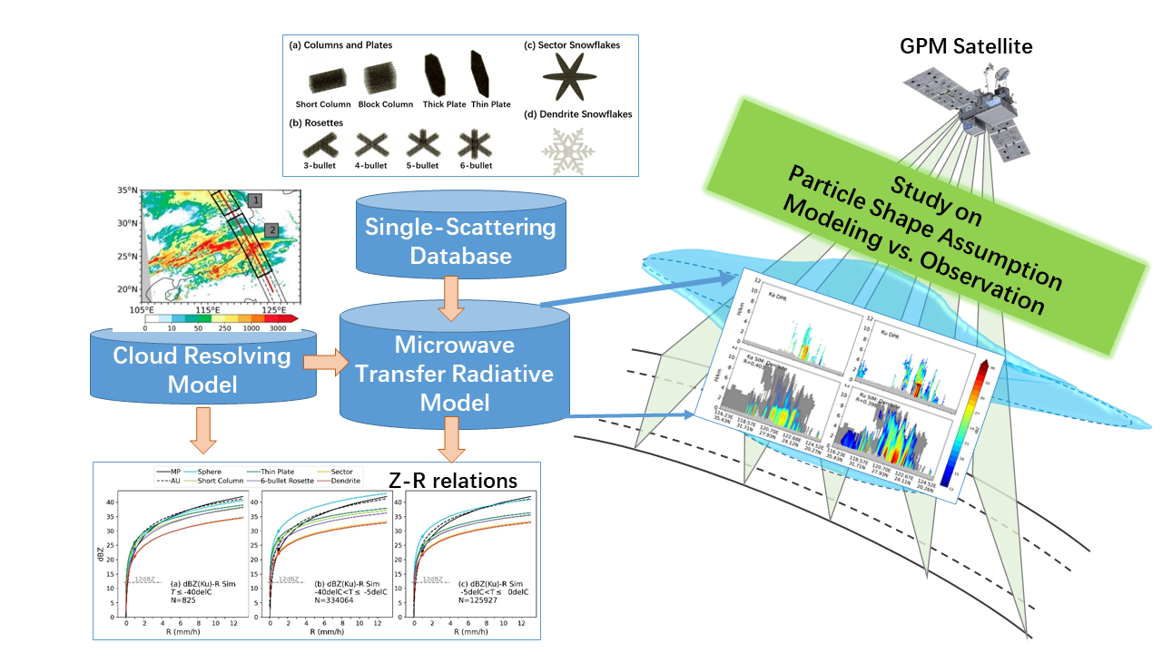
Impacts of Shape Assumptions on Z–R Relationship and Satellite Remote Sensing Clouds Based on Model Simulations and GPM Observations

Abstract
:
1. Introduction
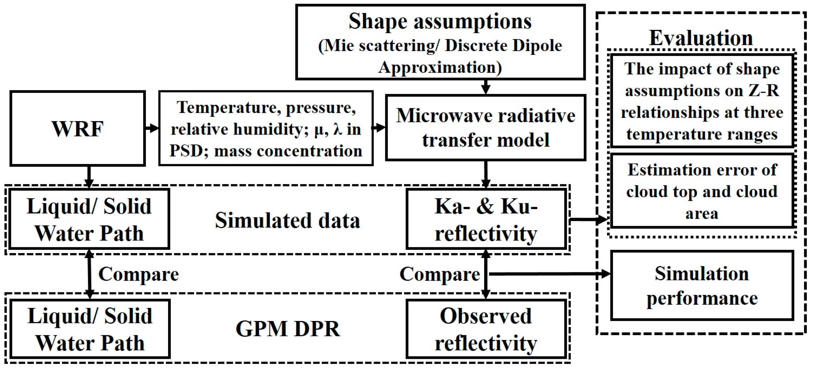
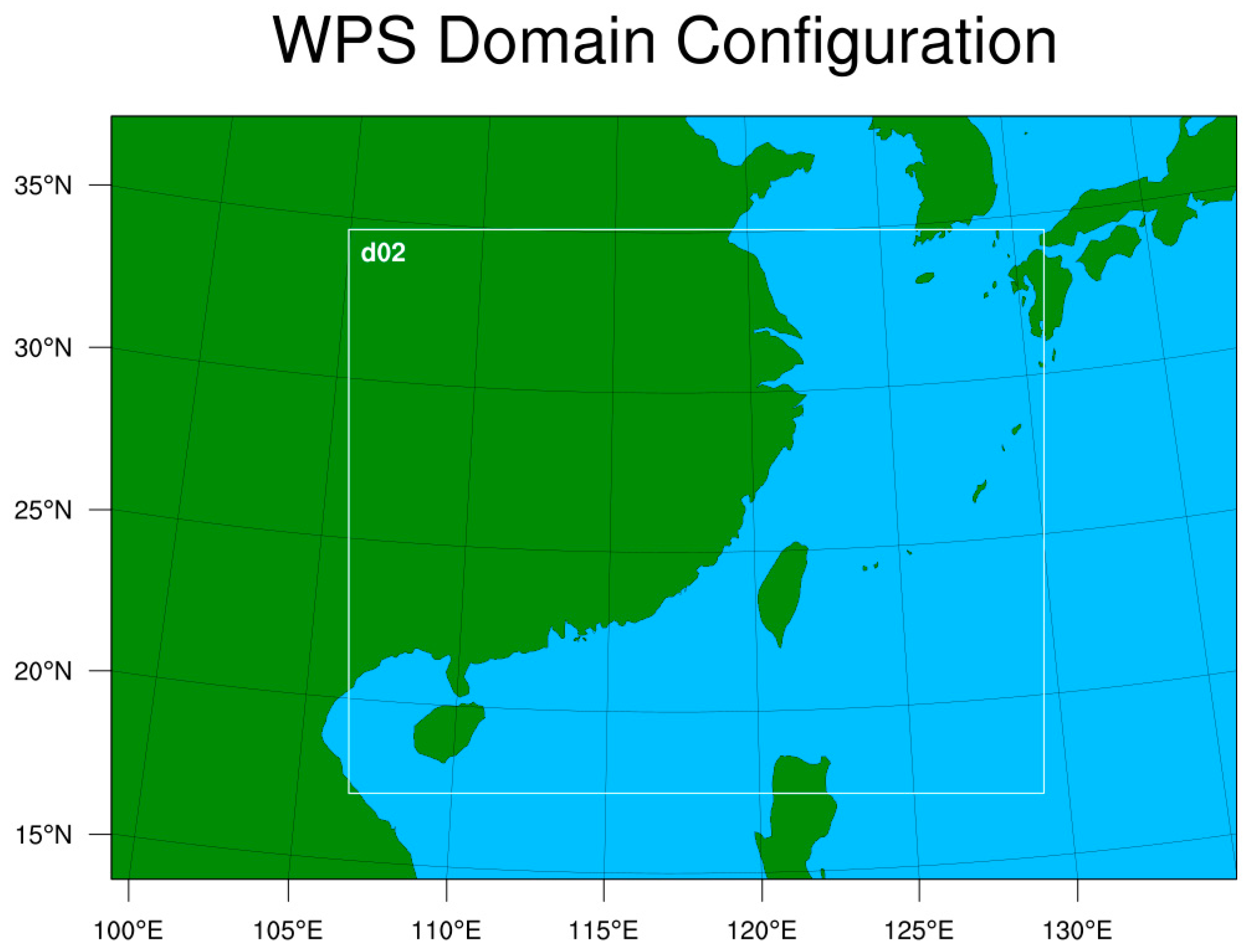
2. Data and Method
3. Results
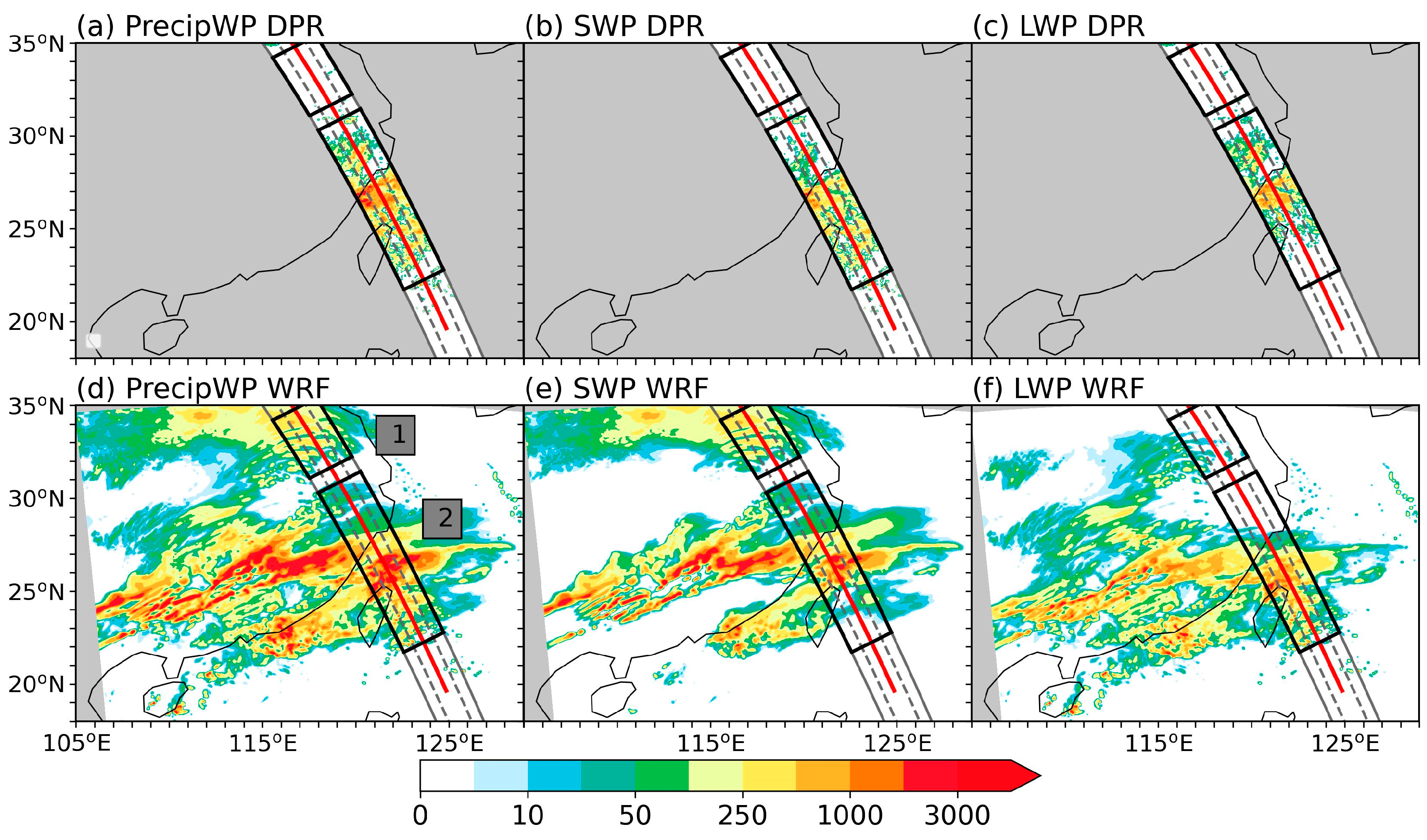
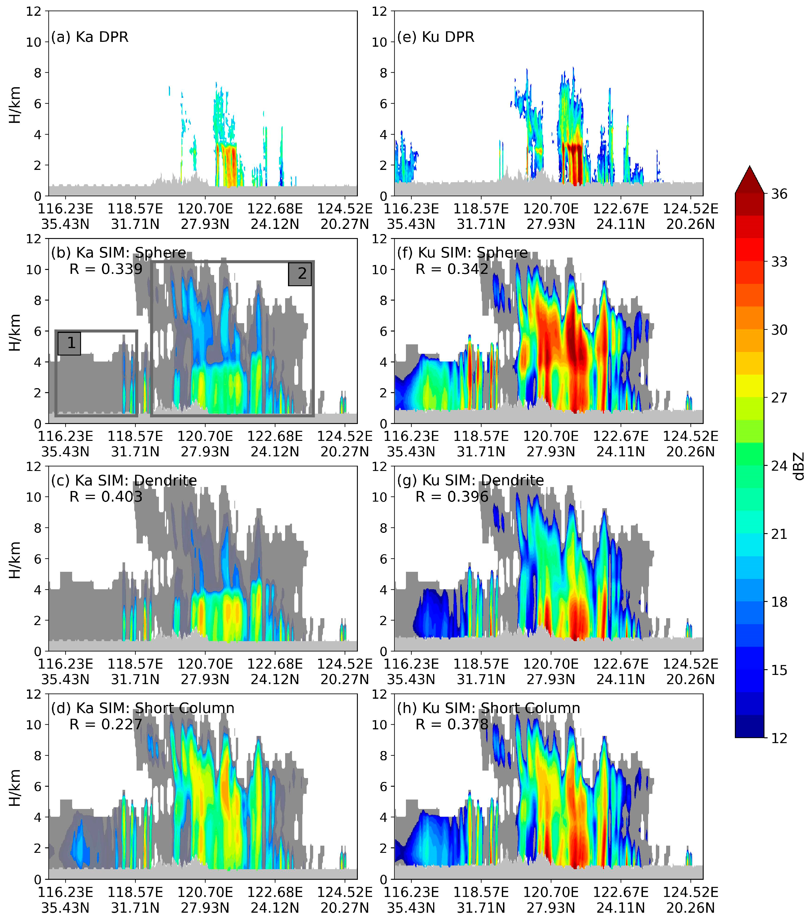
3.1. Correctness of Simulation
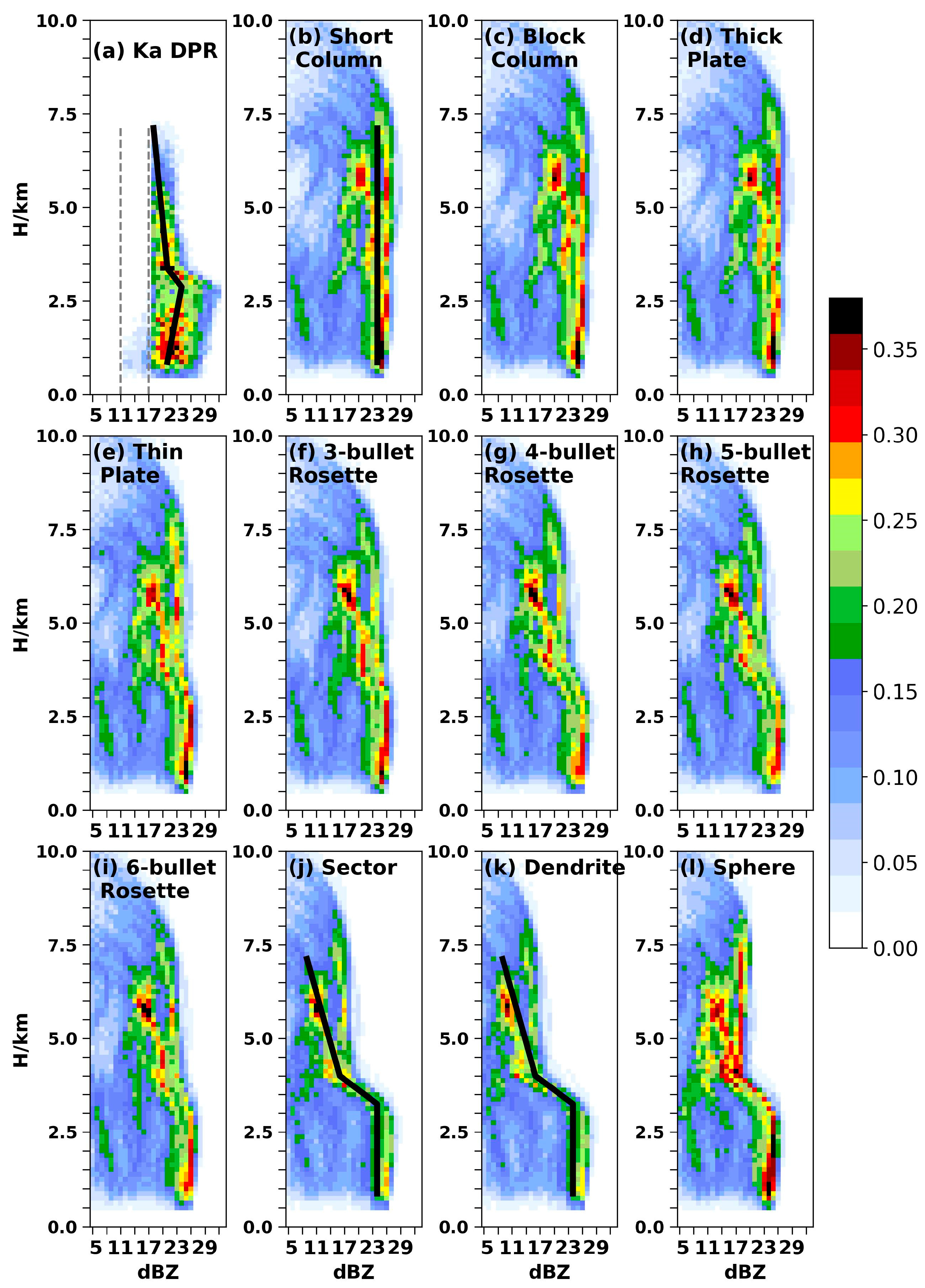
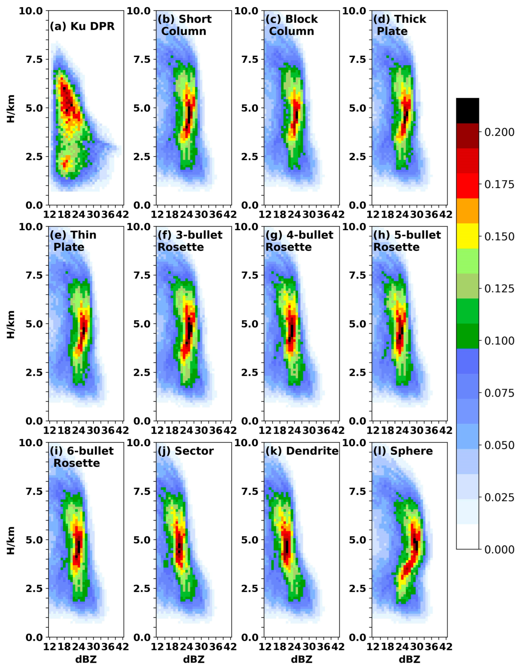
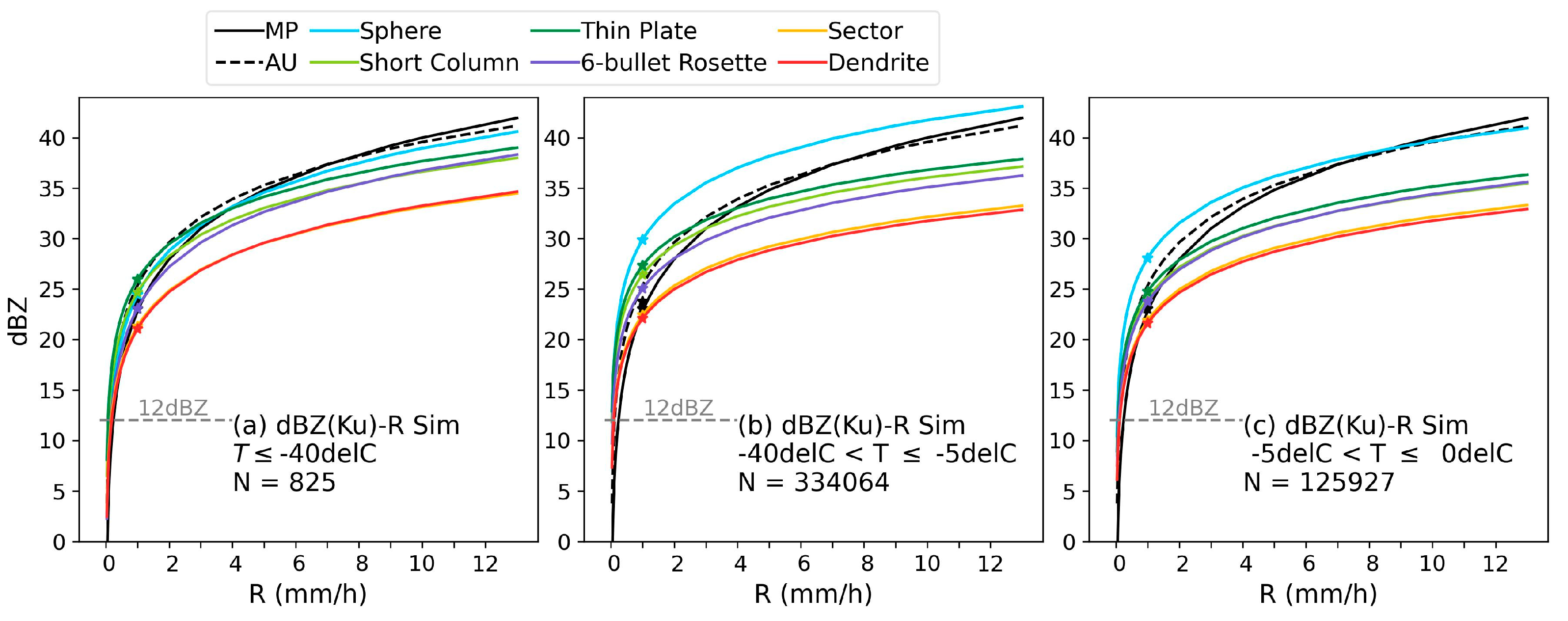
3.2. The Impact of Shape Assumptions on Z–R Relationships in Three Temperature Ranges
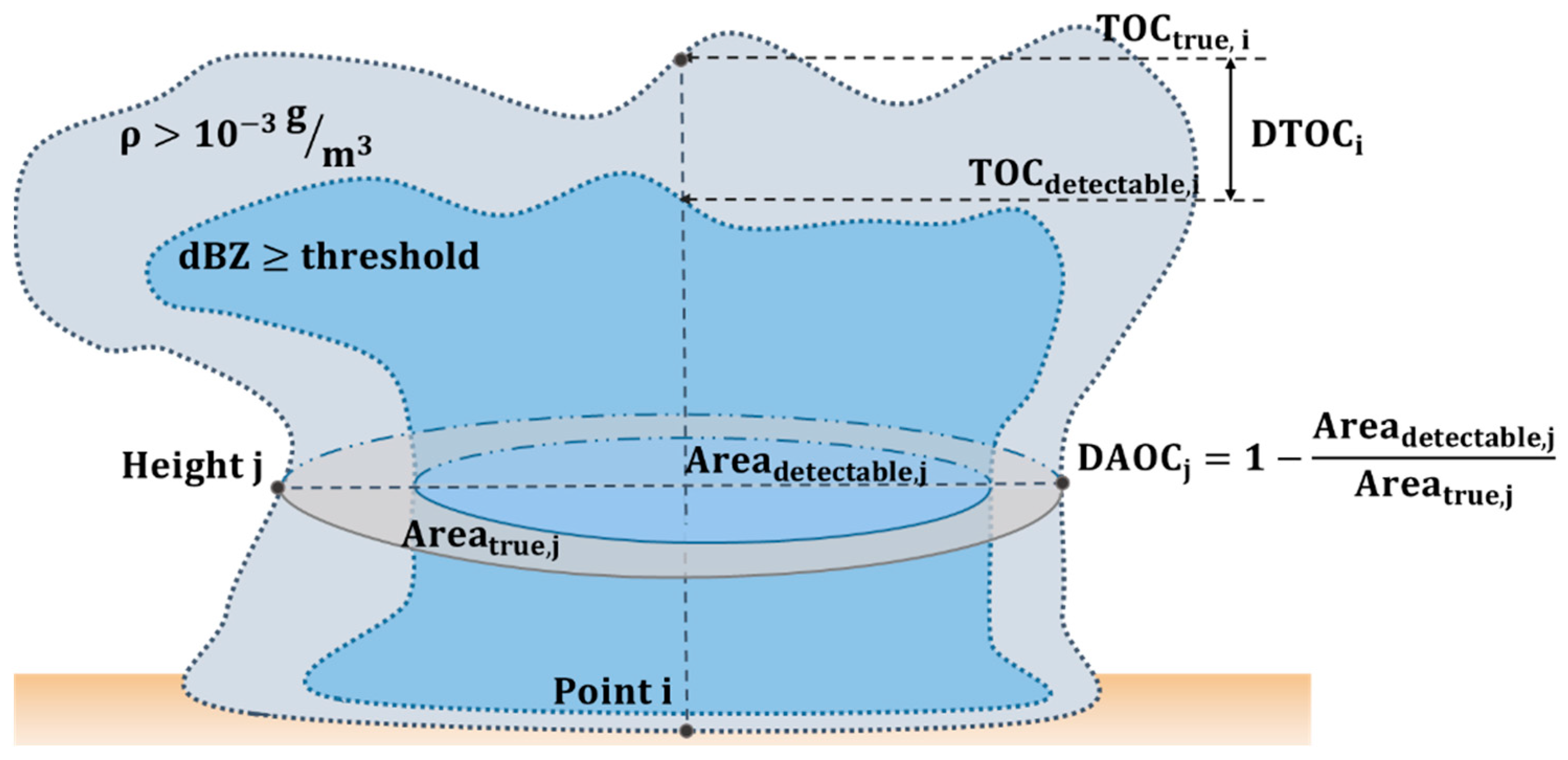
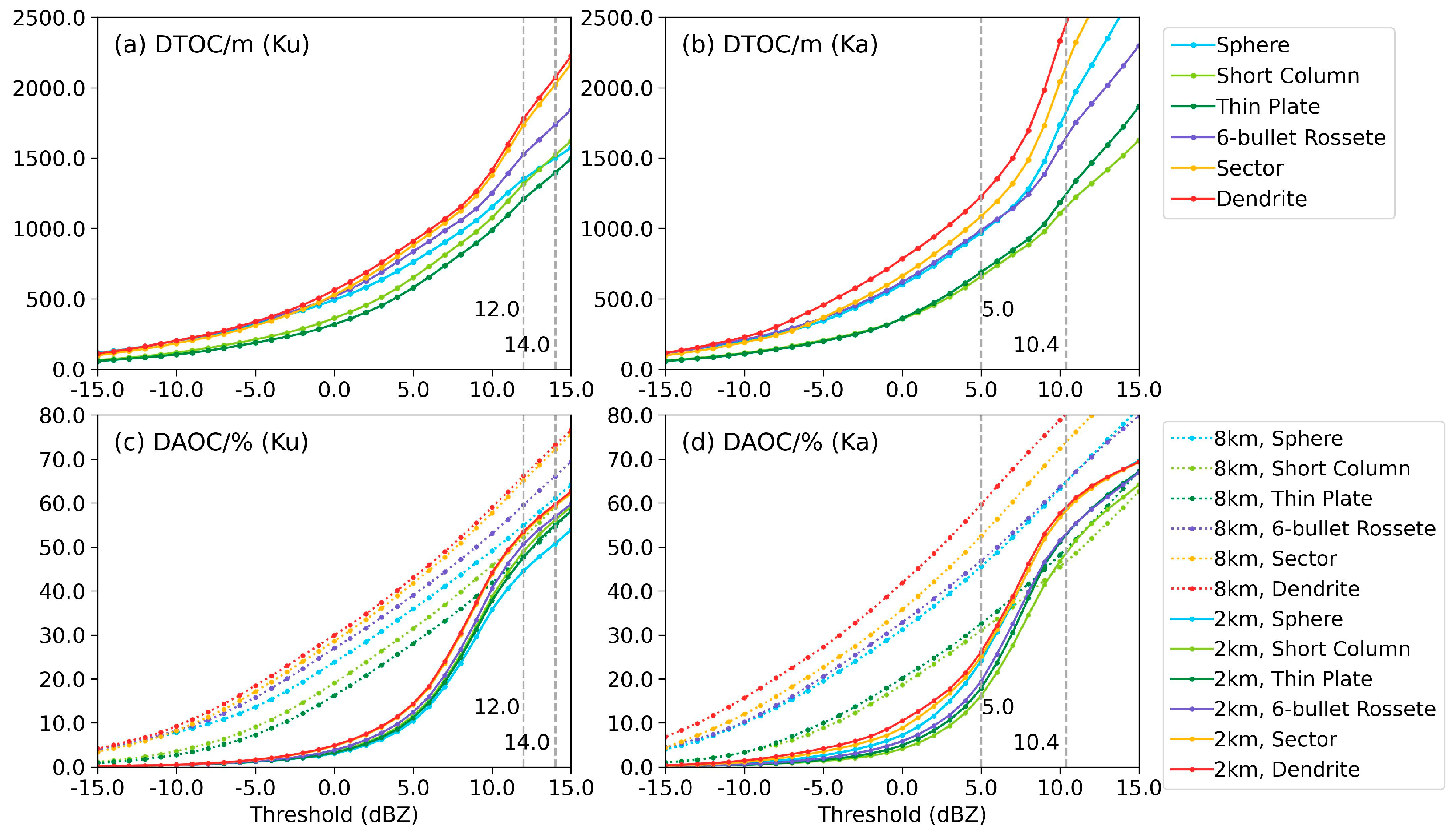
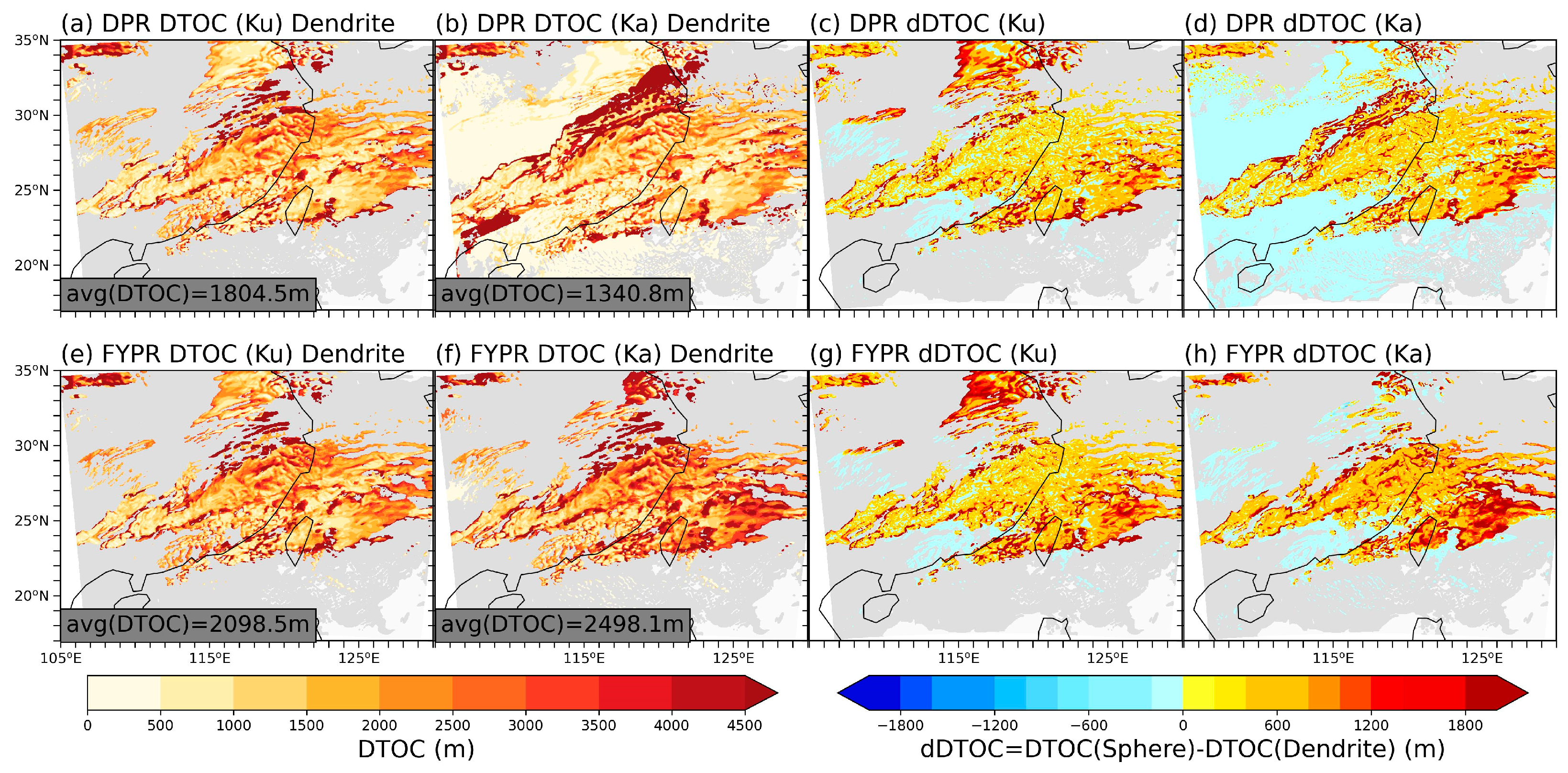
3.3. Estimation Error of Cloud Top and Cloud Area
4. Discussion
5. Conclusions
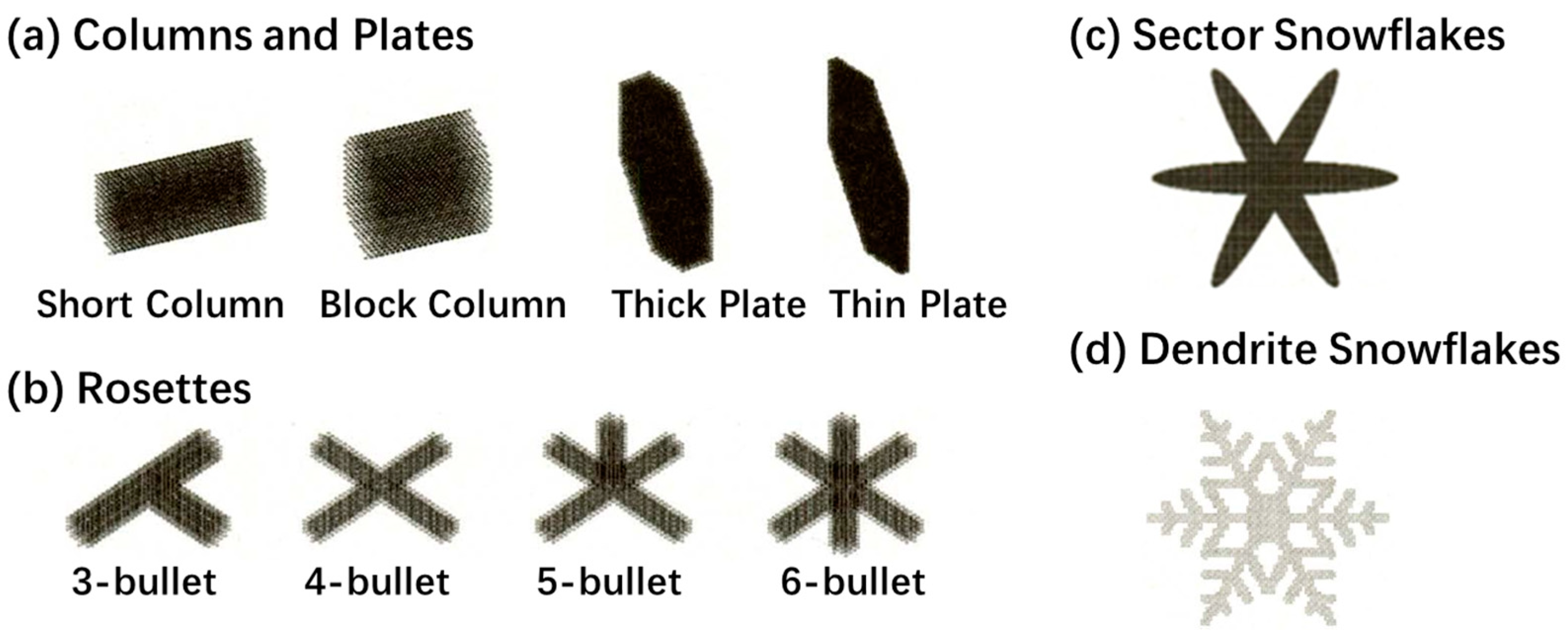
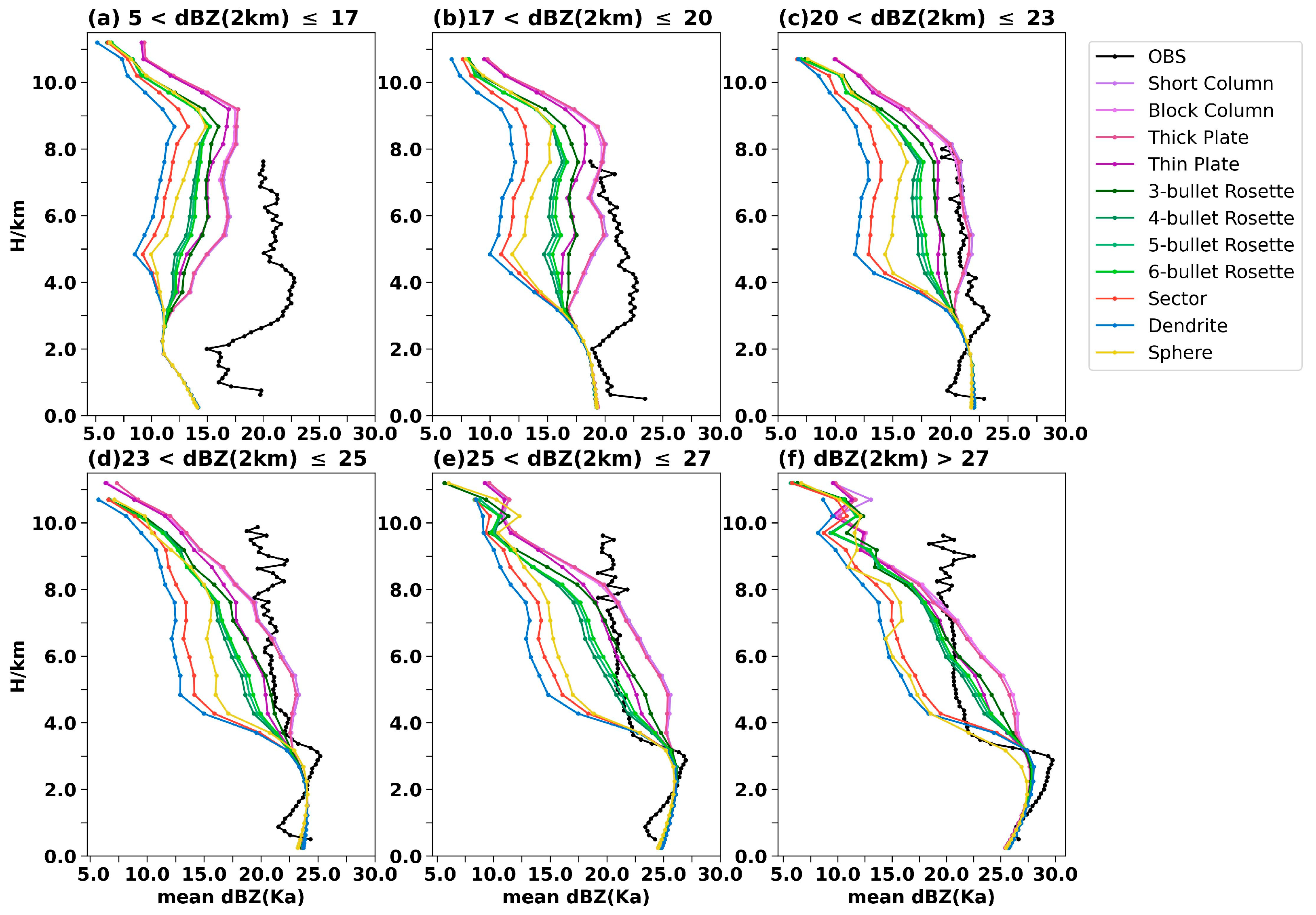
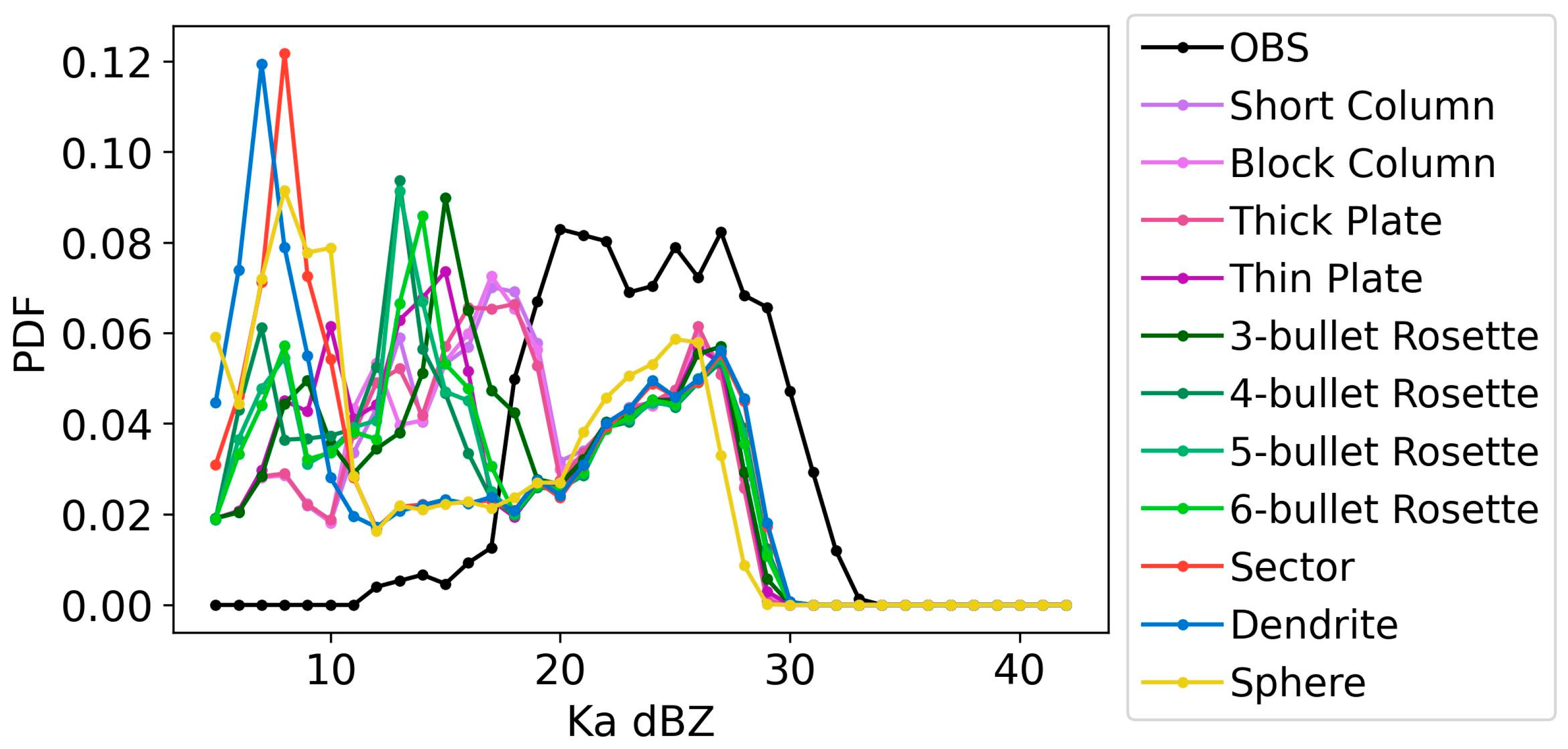
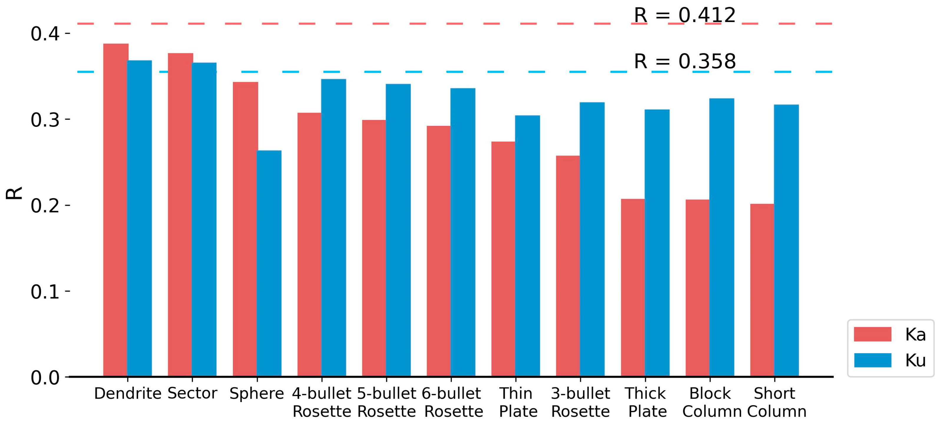
- Compared with the simple-shape assumptions, our complex-shape assumptions (sector and dendrite) performed better in both Ka-band and Ku-band reflectivity simulations. This was shown by the higher correlation coefficients between the simulated and observed reflectivity and smaller differences between their reflectivity profiles. Therefore, snowflakes in the real atmosphere might be closer to sector and dendrite than sphere. The Z–R relationships for these shape assumptions under −40 °C are (sector) and (dendrite). However, snowflakes tend to exist in simple shapes when temperature is low and in complex shapes when temperature is high. The temperature-dependent assumption performs well, especially at Ka-band, but the operational method still needs further study.
- In most conditions, the theoretical Z–R relationships (MP/AU relationships) differed from the fitted Z–R relationships of snowflakes, regardless of their shape. Furthermore, the differences led to estimation errors that stemmed from using a theoretical relationship in the retrieval algorithm. The errors were to underestimate large snowfalls with simple-shaped snowflakes below −40 °C or with complex shapes, and to overestimate snowfalls with spherical snowflakes or small snowfalls with simple-shaped snowflakes below −40 °C.
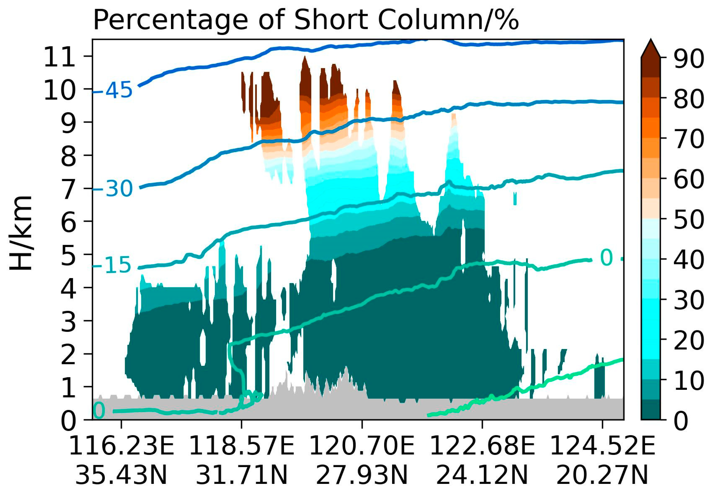
- Under the existing detection sensitivity, the DTOCs of DPR for this case were 1804.5 m (Ka) and 1340.8 m (Ku), and the DAOCs reached 50% and 20% at heights of 8 km and 2 km for Ka-band. If the detection threshold of spaceborne dual frequency radar could reach 5 dBZ (Ku)/0 dBZ (Ka), its detection capability for snowfall in eastern China would be greatly improved.
- An inappropriate shape assumption affected the estimation of detection error: the DTOC of a complex-shape assumption was 200–400 m larger than that of the spherical-shape assumption, while the DAOC was ~15% larger.
Supplementary Materials
Author Contributions
Funding
Data Availability Statement
Acknowledgments
Conflicts of Interest
References
- Trenberth, K.E.; Fasullo, J.T.; Kiehl, J. Earth’s global energy budget. Bull. Am. Meteorol. Soc. 2009, 90, 311–324. [Google Scholar] [CrossRef] [Green Version]
- Stephens, G.L.; Li, J.; Wild, M.; Clayson, C.A.; Loeb, N.; Kato, S.; L’ecuyer, T.; Stackhouse, P.W.; Lebsock, M.; Andrews, T. An update on Earth’s energy balance in light of the latest global observations. Nat. Geosci. 2012, 5, 691–696. [Google Scholar] [CrossRef]
- Budyko, M.I. The heat balance of the earth’s surface. Sov. Geogr. 1961, 2, 3–13. [Google Scholar] [CrossRef]
- Iguchi, T.; Kozu, T.; Meneghini, R.; Awaka, J.; Okamoto, K.I. Rain-Profiling algorithm for the TRMM precipitation radar. J. Appl. Meteorol. 2000, 39, 2038–2052. [Google Scholar] [CrossRef]
- Iguchi, T.; Kozu, T.; Kwiatkowski, J.; Meneghini, R.; Awaka, J.; Okamoto, K.I. Uncertainties in the rain profiling algorithm for the TRMM precipitation radar. J. Meteorol. Soc. Japan. Ser. II 2009, 87, 1–30. [Google Scholar] [CrossRef] [Green Version]
- Kummerow, C.; Barnes, W.; Kozu, T.; Shiue, J.; Simpson, J. The tropical rainfall measuring mission (TRMM) sensor package. J. Atmos. Ocean. Technol. 1998, 15, 809–817. [Google Scholar] [CrossRef]
- Skofronick-Jackson, G.; Kulie, M.; Milani, L.; Munchak, S.J.; Wood, N.B.; Levizzani, V. Satellite Estimation of Falling Snow: A Global Precipitation Measurement (GPM) Core Observatory Perspective. J. Appl. Meteorol. Climatol. 2019, 58, 1429–1448. [Google Scholar] [CrossRef]
- Liao, L.; Meneghini, R. GPM DPR Retrievals: Algorithm, Evaluation, and Validation. Remote Sens. 2022, 14, 843. [Google Scholar] [CrossRef]
- Neeck, S.P.; Kakar, R.K.; Azarbarzin, A.A.; Hou, A.Y. Global Precipitation Measurement (GPM) launch, commissioning, and early operations. In Proceedings of the Sensors, Systems, and Next-Generation Satellites XVIII, Amsterdam, The Netherlands, 22–25 September 2014; pp. 31–44. [Google Scholar]
- Lock, J.A.; Gouesbet, G. Generalized Lorenz–Mie theory and applications. J. Quant. Spectrosc. Radiat. Transf. 2009, 110, 800–807. [Google Scholar] [CrossRef]
- Wriedt, T. Mie theory: A review. In The Mie Theory; Springer: Berlin/Heidelberg, Germany, 2012; pp. 53–71. [Google Scholar]
- Liu, G. Approximation of single scattering properties of ice and snow particles for high microwave frequencies. J. Atmos. Sci. 2004, 61, 2441–2456. [Google Scholar] [CrossRef]
- Liu, G. A Database of Microwave Single-Scattering Properties for Nonspherical Ice Particles. Bull. Am. Meteorol. Soc. 2008, 89, 1563–1570. [Google Scholar] [CrossRef] [Green Version]
- Yang, J.; Weng, F. Analysis of Microwave scattering properties of non-spherical ice particles using discrete dipole approximation. In Proceedings of the IGARSS 2020-2020 IEEE International Geoscience and Remote Sensing Symposium, Waikoloa, HI, USA, 26 September–2 October 2020; pp. 5309–5312. [Google Scholar]
- Xu, X.; Zheng, G.; Wang, Z.; Wang, Q. Experimental and theoretical analyses on the microwave backscattering ability and differential radar reflectivity of nonspherical hydrometeors. J. Quant. Spectrosc. Radiat. Transf. 2005, 92, 61–72. [Google Scholar]
- Kuo, K.-S.; Olson, W.S.; Johnson, B.T.; Grecu, M.; Tian, L.; Clune, T.L.; van Aartsen, B.H.; Heymsfield, A.J.; Liao, L.; Meneghini, R. The microwave radiative properties of falling snow derived from nonspherical ice particle models. Part I: An extensive database of simulated pristine crystals and aggregate particles, and their scattering properties. J. Appl. Meteorol. Climatol. 2016, 55, 691–708. [Google Scholar] [CrossRef]
- Lu, Y.; Jiang, Z.; Aydin, K.; Verlinde, J.; Clothiaux, E.E.; Botta, G. A polarimetric scattering database for nonspherical ice particles at microwave wavelengths. Atmos. Meas. Tech. 2016, 9, 5119–5134. [Google Scholar] [CrossRef] [Green Version]
- Petty, G.W.; Huang, W. Microwave backscatter and extinction by soft ice spheres and complex snow aggregates. J. Atmos. Sci. 2010, 67, 769–787. [Google Scholar] [CrossRef]
- Olson, W.S.; Tian, L.; Grecu, M.; Kuo, K.-S.; Johnson, B.T.; Heymsfield, A.J.; Bansemer, A.; Heymsfield, G.M.; Wang, J.R.; Meneghini, R. The microwave radiative properties of falling snow derived from nonspherical ice particle models. Part II: Initial testing using radar, radiometer and in situ observations. J. Appl. Meteorol. Climatol. 2016, 55, 709–722. [Google Scholar] [CrossRef]
- Johnson, B.; Skofronick-Jackson, G. The influence of non-spherical particles and land surface emissivity on combined radar/radiometer precipitation retrievals. In Proceedings of the EGU General Assembly Conference Abstracts, Vienna, Austria, 19–24 April 2009; p. 6151. [Google Scholar]
- Baran, A.J. A review of the light scattering properties of cirrus. J. Quant. Spectrosc. Radiat. Transf. 2009, 110, 1239–1260. [Google Scholar]
- Baran, A.J. From the single-scattering properties of ice crystals to climate prediction: A way forward. Atmos. Res. 2012, 112, 45–69. [Google Scholar] [CrossRef]
- Field, P.; Hogan, R.; Brown, P.; Illingworth, A.; Choularton, T.; Cotton, R. Parametrization of ice-particle size distributions for mid-latitude stratiform cloud. Q. J. R. Meteorol. Soc. J. Atmos. Sci. Appl. Meteorol. Phys. Oceanogr. 2005, 131, 1997–2017. [Google Scholar]
- Heymsfield, A.J.; Platt, C. A parameterization of the particle size spectrum of ice clouds in terms of the ambient temperature and the ice water content. J. Atmos. Sci. 1984, 41, 846–855. [Google Scholar] [CrossRef]
- Connolly, P.; Saunders, C.; Gallagher, M.; Bower, K.; Flynn, M.; Choularton, T.; Whiteway, J.; Lawson, R. Aircraft observations of the influence of electric fields on the aggregation of ice crystals. Q. J. R. Meteorol. Soc. J. Atmos. Sci. Appl. Meteorol. Phys. Oceanogr. 2005, 131, 1695–1712. [Google Scholar] [CrossRef]
- Bailey, M.; Hallett, J. Growth rates and habits of ice crystals between −20° and−70 °C. J. Atmos. Sci. 2004, 61, 514–544. [Google Scholar] [CrossRef]
- Saha, S.; Niranjan Kumar, K.; Sharma, S.; Kumar, P.; Joshi, V. Can Quasi-Periodic Gravity Waves Influence the Shape of Ice Crystals in Cirrus Clouds? Geophys. Res. Lett. 2020, 47, e2020GL087909. [Google Scholar] [CrossRef]
- Heymsfield, A.J.; Miloshevich, L.M. Parameterizations for the cross-sectional area and extinction of cirrus and stratiform ice cloud particles. J. Atmos. Sci. 2003, 60, 936–956. [Google Scholar] [CrossRef]
- Gallagher, M.W.; Connolly, P.; Whiteway, J.; Figueras-Nieto, D.; Flynn, M.; Choularton, T.; Bower, K.; Cook, C.; Busen, R.; Hacker, J. An overview of the microphysical structure of cirrus clouds observed during EMERALD-1. Q. J. R. Meteorol. Soc. J. Atmos. Sci. Appl. Meteorol. Phys. Oceanogr. 2005, 131, 1143–1169. [Google Scholar] [CrossRef] [Green Version]
- Kintea, D.M.; Hauk, T.; Roisman, I.V.; Tropea, C. Shape evolution of a melting nonspherical particle. Phys. Rev. E 2015, 92, 033012. [Google Scholar] [CrossRef] [Green Version]
- Pan, D.; Liu, L.-M.; Slater, B.; Michaelides, A.; Wang, E. Melting the ice: On the relation between melting temperature and size for nanoscale ice crystals. ACS Nano 2011, 5, 4562–4569. [Google Scholar] [CrossRef]
- Johnson, B.; Olson, W.; Skofronick-Jackson, G. The microwave properties of simulated melting precipitation particles: Sensitivity to initial melting. Atmos. Meas. Tech. 2016, 9, 9–21. [Google Scholar] [CrossRef] [Green Version]
- Kulie, M.S.; Bennartz, R.; Greenwald, T.J.; Chen, Y.; Weng, F. Uncertainties in microwave properties of frozen precipitation: Implications for remote sensing and data assimilation. J. Atmos. Sci. 2010, 67, 3471–3487. [Google Scholar] [CrossRef] [Green Version]
- Hong, G. Parameterization of scattering and absorption properties of nonspherical ice crystals at microwave frequencies. J. Geophys. Res. Atmos. 2007, 112. [Google Scholar] [CrossRef]
- Leinonen, J.; Kneifel, S.; Moisseev, D.; Tyynelä, J.; Tanelli, S.; Nousiainen, T. Evidence of nonspheroidal behavior in millimeter-wavelength radar observations of snowfall. J. Geophys. Res. Atmos. 2012, 117. [Google Scholar] [CrossRef] [Green Version]
- Kulie, M.S.; Hiley, M.J.; Bennartz, R.; Kneifel, S.; Tanelli, S. Triple-frequency radar reflectivity signatures of snow: Observations and comparisons with theoretical ice particle scattering models. J. Appl. Meteorol. Climatol. 2014, 53, 1080–1098. [Google Scholar] [CrossRef] [Green Version]
- Wang, Y.; Han, T.; Guo, J.; Jiang, K.; Li, R.; Shao, W.; Liu, G. Simulation of three-dimensional structure of cloud and rain detected by Ku, Ka and W radar. Sci. Bull. 2019, 64, 430–443. [Google Scholar]
- Draine, B.T.; Flatau, P.J. User Guide for the Discrete Dipole Approximation Code DDSCAT, Version 5a10. Available online: https://arxiv.org/abs/astro-ph/0008151 (accessed on 7 March 2023).
- Tokay, A.; Short, D.A. Evidence from tropical raindrop spectra of the origin of rain from stratiform versus convective clouds. J. Appl. Meteorol. Climatol. 1996, 35, 355–371. [Google Scholar] [CrossRef]
- Casella, D.; Panegrossi, G.; Sanò, P.; Marra, A.C.; Dietrich, S.; Johnson, B.T.; Kulie, M.S. Evaluation of the GPM-DPR snowfall detection capability: Comparison with CloudSat-CPR. Atmos. Res. 2017, 197, 64–75. [Google Scholar] [CrossRef]
- Heymsfield, A.; Bansemer, A.; Wood, N.B.; Liu, G.; Tanelli, S.; Sy, O.O.; Poellot, M.; Liu, C. Toward improving ice water content and snow-rate retrievals from radars. Part II: Results from three wavelength radar–collocated in situ measurements and CloudSat–GPM–TRMM radar data. J. Appl. Meteorol. Climatol. 2018, 57, 365–389. [Google Scholar] [CrossRef]
- Mroz, K.; Montopoli, M.; Battaglia, A.; Panegrossi, G.; Kirstetter, P.; Baldini, L. Cross validation of active and passive microwave snowfall products over the continental United States. J. Hydrometeorol. 2021, 22, 1297–1315. [Google Scholar] [CrossRef]
- Zhou, R.; Yan, T.; Yang, S.; Fu, Y.; Huang, C.; Zhu, H.; Li, R. Characteristics of clouds, precipitation, and latent heat in midlatitude frontal system mixed with dust storm from GPM satellite observations and WRF simulations. JUSTC 2022, 52, 3-1–3-15. [Google Scholar] [CrossRef]
- Iguchi, T.; Meneghini, R. Intercomparison of single-frequency methods for retrieving a vertical rain profile from airborne or spaceborne radar data. J. Atmos. Ocean. Technol. 1994, 11, 1507–1516. [Google Scholar] [CrossRef]
- Marshall, J.; Palmer, W.M. Shorter Contributions. J. Meteorol. 1948, 5, 166. [Google Scholar]
- Ulbrich, C.W.; Atlas, D. A method for measuring precipitation parameters using radar reflectivity and optical extinction. Ann. Des. Télécommunications 1977, 415–421. [Google Scholar] [CrossRef]
- Uijlenhoet, R. Raindrop size distributions and radar reflectivity–rain rate relationships for radar hydrology. Hydrol. Earth Syst. Sci. 2001, 5, 615–628. [Google Scholar] [CrossRef] [Green Version]


| Domain ID | 01 | 02 |
|---|---|---|
| Lateral/initial data | CFSv2 6 hourly | |
| MP physics | Morrison | |
| CU physics | Modified Tiedtke scheme | None |
| Boundary layer physics | Mellor–Yamada–Janjic TKE scheme | |
| Surface layer physics | Monin–Obukhov (Janjic) scheme | |
| Land surface physics | Unified Noah land-surface model | |
| Longwave radiation physics | RRTMG scheme | |
| Shortwave radiation physics | RRTMG scheme | |
| Time step | 60 s | 20 s |
| Spatial resolution | 12 km | 4 km |
| Time range | 1 January 2018–8 January 2018 | |
| Output interval | None | 30 min |
| Feedback | False | |
| Temperature | Sphere | Short Column | Thin Plate | 6-Bullet Rosette | Sector | Dendrite |
|---|---|---|---|---|---|---|
| T ≤ −40 °C | 0.18 | 0.04 | 0.03 | 0.12 | 0.03 | 0.05 |
| −40 < T ≤ −5 °C | 4.14 | 0.88 | 0.74 | 0.78 | 0.27 | 0.28 |
| −5 < T ≤ 0 °C | 22.72 | 11.19 | 12.82 | 8.07 | 4.53 | 4.25 |
| Parameters | Temperature/°C | Sphere | Short Column | Thin Plate | 6-Bullet Rosette | Sector | Dendrite |
|---|---|---|---|---|---|---|---|
| A | T ≤ −40 | 24.43 | 24.68 | 25.96 | 23.08 | 21.29 | 21.05 |
| −40 < T ≤ −5 | 29.88 | 26.43 | 27.33 | 25.03 | 22.41 | 22.07 | |
| −5 < T ≤ 0 | 28.07 | 24.10 | 24.76 | 23.74 | 21.88 | 21.60 | |
| B | T ≤ −40 | 14.51 | 11.95 | 11.72 | 13.68 | 11.84 | 12.21 |
| −40 < T ≤ −5 | 11.85 | 9.61 | 9.48 | 10.06 | 9.74 | 9.67 | |
| −5 < T ≤ 0 | 11.57 | 10.21 | 10.39 | 10.65 | 10.27 | 10.17 |
Disclaimer/Publisher’s Note: The statements, opinions and data contained in all publications are solely those of the individual author(s) and contributor(s) and not of MDPI and/or the editor(s). MDPI and/or the editor(s) disclaim responsibility for any injury to people or property resulting from any ideas, methods, instructions or products referred to in the content. |
© 2023 by the authors. Licensee MDPI, Basel, Switzerland. This article is an open access article distributed under the terms and conditions of the Creative Commons Attribution (CC BY) license (https://creativecommons.org/licenses/by/4.0/).
Share and Cite
Mai, L.; Yang, S.; Wang, Y.; Li, R. Impacts of Shape Assumptions on Z–R Relationship and Satellite Remote Sensing Clouds Based on Model Simulations and GPM Observations. Remote Sens. 2023, 15, 1556. https://doi.org/10.3390/rs15061556
Mai L, Yang S, Wang Y, Li R. Impacts of Shape Assumptions on Z–R Relationship and Satellite Remote Sensing Clouds Based on Model Simulations and GPM Observations. Remote Sensing. 2023; 15(6):1556. https://doi.org/10.3390/rs15061556
Chicago/Turabian StyleMai, Liting, Shuping Yang, Yu Wang, and Rui Li. 2023. "Impacts of Shape Assumptions on Z–R Relationship and Satellite Remote Sensing Clouds Based on Model Simulations and GPM Observations" Remote Sensing 15, no. 6: 1556. https://doi.org/10.3390/rs15061556