Article

Development and Application of Predictive Models to Distinguish Seepage Slicks from Oil Spills on Sea Surfaces Employing SAR Sensors and Artificial Intelligence: Geometric Patterns Recognition under a Transfer Learning Approach

by
Patrícia Carneiro Genovez
1,*,
Francisco Fábio de Araújo Ponte
1,
Ítalo de Oliveira Matias
1,
Sarah Barrón Torres
1,
Carlos Henrique Beisl
2,
Manlio Fernandes Mano
3,
Gil Márcio Avelino Silva
4 and
Fernando Pellon de Miranda
4
1
Software Engineering Laboratory (LES), Informatics Division, Pontifical Catholic University of Rio de Janeiro (PUC-Rio), R. Marquês de São Vicente, 225—Gávea, Rio de Janeiro 22451-900, Brazil
2
GeoSpatial Petroleum, R. Miguel de Farias, 92, Icaraí, Niterói, Rio de Janeiro 24220-002, Brazil
3
Oil Finder, R. Voluntários da Pátria, 48, Botafogo, Rio de Janeiro 22270-000, Brazil
4
Petrobras Research, Development and Innovation Center (CENPES), Federal University of Rio de Janeiro, Av. Horácio Macedo 950, Cidade Universitária, Ilha do Fundão, Rio de Janeiro 21941-915, Brazil
*
Author to whom correspondence should be addressed.
Remote Sens. 2023, 15(6), 1496; https://doi.org/10.3390/rs15061496
Submission received: 7 February 2023 / Revised: 27 February 2023 / Accepted: 2 March 2023 / Published: 8 March 2023
(This article belongs to the Special Issue Added-Value SAR Products for the Observation of Coastal Areas)

Abstract

:
The development and application of predictive models to distinguish seepage slicks from oil spills are challenging, since Synthetic Aperture Radars (SAR) detect these events as dark spots on the sea surface. Traditional Machine Learning (ML) has been used to discriminate the Oil Slick Source (OSS) as natural or anthropic assuming that the samples employed to train and test the models in the source domain (DS) follow the same statistical distribution of unknown samples to be predicted in the target domain (DT). When such assumptions are not held, Transfer Learning (TL) allows the extraction of knowledge from validated models and the prediction of new samples, thus improving performances even in scenarios never seen before. A database with 26 geometric features extracted from 6279 validated oil slicks was used to develop predictive models in the Gulf of Mexico (GoM) and its Mexican portion (GMex). Innovatively, these well-trained models were applied to predict the OSS of unknown events in the GoM, the American (GAm) portion of the GoM, and in the Brazilian continental margin (BR). When the DS and DT domains are similar, the TL and generalization are null, being equivalent to the usual ML. However, when domains are different but statically related, TL outdoes ML (58.91%), attaining 87% of global accuracy when using compatible SAR sensors in the DS and DT domains. Conversely, incompatible SAR sensors produce domains statistically divergent, causing negative transfers and generalizations. From an operational standpoint, the evidenced generalization capacity of these models to recognize geometric patterns across different geographic regions using TL may allow saving time and budget, avoiding the collection of validated and annotated new training samples, as well as the models re-training from scratch. When looking for new exploratory frontiers, automatic prediction is a value-added product that strengthens the knowledge-driven classifications and the decision-making processes. Moreover, the prompt identification of an oil spill can speed up the response actions to clean up and protect sensitive areas against oil pollution.

1. Introduction

Petrogenic oil slicks can reach the sea surface seeping naturally from the seafloor by migration through geological faults connected with source rocks [1,2,3,4,5]. They can also be intentionally or accidentally discharged from offshore petroleum infrastructures, or from other human sources such as shipping or land-based runoff [6,7,8]. A recent global-scale effort to understand the sources of chronic oiling in the oceans demonstrated that most oil slicks come from human actions [8]. Regardless of whether the source is natural or anthropic, crude oil and its derived products contain persistent and toxic compounds that represent an imminent risk for marine ecosystems, bringing adverse short, medium, and long-term environment and socio-economic impacts [1,9].
From this perspective, Earth Observation (EO) data assume an important role providing spatially and temporally consistent information for systematically monitoring the oceans [10,11]. The expressive availability of free EO products, and the effectiveness of powerful learning algorithms, combined with high-performance computing advances, bring unprecedented opportunities to develop automatic expert systems supporting data-driven decisions [10,11,12].
Remarkably, Synthetic Aperture Radars (SAR) are key-operational data providers for oil pollution monitoring offering a synoptic view over affected sites in near-real-time, as well as acquiring images during day and night regardless of weather conditions [6,7,13,14,15]. In the microwave spectrum, natural or anthropic oil slicks induce the same physical mechanism of damping sea surface roughness, being similarly detected as dark spots, i.e., regions with low backscattering coefficients [2,15,16,17,18,19,20,21].
Particularly, the use of SAR data to detect likely seepage slicks on sea surfaces represents an important instrument for reducing exploratory risk [4,5,22], as well as for protecting petroleum companies against penalties by events, not human-induced [22]. The location and persistence of detected slicks can be correlated with inverse oil drifting models [23,24], 3D-seismic and other remotely sensed geophysical data increasing confidence and strengthening evidence of active petroleum systems. This possibility allows for searching new exploratory frontiers in deep to ultra-deepwater, as well as provides ancillary information for decision-making facing time and budget restrictions [4].
Since the nineties [18,25,26,27,28,29,30,31,32,33,34,35,36,37,38,39], Machine Learning (ML) has provided a fundamental contribution in developing expert systems designed for oil slick detection and discrimination from other similar phenomena also known as look-alikes. Historically, the architecture of these systems uses as a basis the discriminatory potential [18,33,34,35,36,37,38,39,40,41] of different radiometric, textural, polarimetric, geometric, and/or contextual handcrafted features extracted from SAR data, following four usual steps [18,37]: (i) SAR pre-processing; (ii) dark spot detection [35,38,39]; (iii) feature extraction and selection [33,34,35,36]; and (iv) oil slick classification. However, the versatility of ML to recognize patterns and learn meaningful and consistent information for predicting the oil slick source (OSS) as natural or anthropic is under investigation [2,22,42,43,44], consolidating a new and important research topic.
Traditional ML algorithms make predictions of unknown data using statistical models trained on previously labelled (supervised) or unlabelled (unsupervised) samples. The common assumption is that the samples employed to train and test the models in the source domain (DS) follow the same statistical distribution of unknown samples to be predicted in the target domain (DT). Under such an approach knowledge is neither retained nor adapted when a new dataset, from a different geographic region with dissimilar statistical properties, is acquired. In this case, classification and regression models need to be rebuilt and retrained from scratch by acquiring new representative and validated samples [11,45,46].
Nevertheless, in real-world applications, when the phenomenon under consideration is rare or unpredictable (e.g., oil spillage or natural seepage), acquiring a huge amount of validated and labelled samples in remote offshore regions is challenging, expensive and often impracticable. In such circumstances, Transfer Learning (TL) represents a solution that makes it possible to extract and store knowledge from robust and validated databases, transferring it to predict new samples from different locations [45,46,47].
TL is a ML’s frontier that aims to improve the generalization ability of well-trained models under controlled domains, adapting them to be applied in different but related domains [48]. TL utilizes labelled data more effectively, reducing the need to collect and annotate new training samples, making the learning process faster and more accurate, therefore avoiding the need to rebuild predictive models from scratch [45].
The proposed objective goes beyond state-of-the-art, unprecedentedly applying robust, validated, and well-trained models to extract knowledge from natural and anthropic oil slicks, transferring it to predict the OSS of unknown samples employing TL. The innovative aspects of this research also embrace the assessment of the generalization capacity of these models to recognize patterns based only on the geometric properties of oil slicks detected in different geographic regions, by distinct satellites, under diverse meteo-oceanographic conditions.
To accomplish these goals, a huge and original database containing geometric patterns extracted from more than 6000 oil slicks detected by multiple SAR sensors in the Gulf of Mexico for 13 years is used as input. This rare and valuable dataset of labelled samples was field validated by PEMEX (Petróleos Mexicanos based on Ciudad del Carmen, Gulf of Mexico) and used to develop trustworthy and controlled predictive models for OSS identification.
With the confirmation of the adaptability of these models to learn geometric patterns and transfer them to make accurate inferences on new samples from different locations, it is possible to save time and budget spent on the acquisition and validation of new samples to build new models, optimizing human resources and infrastructure.
Furthermore, a critical point in intersectoral Research, Development, and Innovation (RD&I) projects integrating academia and the private sector is to generate positive returns on the investments carried out to develop ML systems [49]. In this sense, this project goes further by foreseeing a broader architecture designed for the operational deployment in the Petrobras proprietary software named GeoqView [22,43,44]. Under a ground-breaking view, the migration from the developer to the production environment combines the data-driven and knowledge-driven approaches, using automatic inferences to strengthen the experts’ interpretation when searching for new exploratory frontiers.
Beyond the theoretical background (Section 1.1 and Section 1.2), the article is organized into four sections encompassing the entire lifecycle of a ML predictive system, as follows: (Section 2) database description and methodology statement; (Section 3) results including the development (Section 3.1) and application (Section 3.2) of the predictive models, as well as an evaluation of their operational feasibility (Section 3.3), deployment and use (Section 3.4). A discussion, conclusion, and reflections regarding the scientific, environmental, and socio-economic impacts of the project outcomes, as well as its future perspective, are pointed out in Section 4 and Section 5.

1.1. Oil Slick Source Identification under a Transfer Learning Approach

Regarding the development and application of predictive models for OSS identification under a TL approach, some important definitions and notations are essential to understand the proposed research. Particularly, the definition of task and domain is the core to extract, learn and transfer knowledge from robust predictive models to unknown datasets.
A domain (D) is composed of two elements, a feature space X, and a marginal probability distribution P(X), where X = {x1, …, xn} Є X. To accomplish the OSS identification task, X represents the space of all instance vectors, where xi is the ith vector corresponding to some oil slick sample, while X refers to a particular subset of learning samples intended for training, testing or validation of the predictive models. Each xi instance within the database is an oil slick represented by a vector compiling 26 geometric features (Section 2.1).
Generally, two domains are defined during the development and application of intelligent systems: the source domain (DS) and the target domain (DT). The source domain (DS) comprises validated and balanced oil slick samples—labelled or not—used for training and testing predictive models, while the target domain (DT) is composed by new samples—labelled or not—to be predicted by the model. Task (T) indicates the purpose of the samples used in the source (TS) and in the target (TT) domains, which can be equal or different, as well as labelled or not [45,48].
More specifically, DS is denoted as DS = {(xS1, yS1), …,(xSn, ySn)}, where each data instance xS Є XS takes an associated label yS Є YS. The dataset in the DT domain represents the unknown samples to be predicted and is similarly denoted as DT = {(xT1, yT1), …,(xTn, yTn)}, where each new input sample xT Є XT will be assigned to one label yT Є YT, indicating its source as natural or anthropic.
Therefore, considering a specific source domain DS = {XS, P(XS)} and a target domain DT = {XT, P(XT)}, a task consists of two components: a label space Y and an objective predictive function fT(·) denoted by T = {Y, fT(·)}. Under a TL approach, the predictive function fT(·) can be learned from the DS domain function fS(·) using the knowledge extracted from pairs of samples {xSi, ySi} employed during the model building. Probabilistically, the function fT(·) is used to predict the corresponding label y of a new instance xT in the DT domain p(yT|x) [48,50].
Given the available database, the TS and TT tasks are the same, comprising a binary classification that aims to assign labels Y Є {0, 1}, where 1 refers to the class seepage slick and 0 to the class oil spill, characterizing the OSS identification task (TOSS).
The way tasks and domains are configured in the source and target will determine the type of transfer learning. There are three settings for TL comprising the inductive, transductive and unsupervised transfer learning, as described below [45,51].
Inductive Transfer Learning occurs when the TS and TT tasks are different (TS ≠ TT) but related, and the DS and DT domains are the same (DS = DT). In this type of TL, labelled data are available for the DT but not necessarily for the DS domain. The availability of labelled data in the DS domain configures a Multi-Task-Learning, and its absence is a Self-Taught-Learning.
Unsupervised Transfer Learning considers different but related tasks (TS ≠ TT) and domains (DS ≠ DT), dealing with no labelled data in both of the DS and DT domains.
Transductive Transfer Learning (TTL) considers the same tasks (TS = TT), and different but related domains (DS ≠ DT). In such a case, a lot of validated and labelled data are available in the DS domain, whereas no labelled data are available in the DT domain. Essentially, TTL aims to adapt the predictive function fS(·) learned from the labelled data (xS) in the DS domain to predict fT(·) unlabelled samples (xT) in the DT domain [45,48]. Differences between the two domains (DS ≠ DT) [45,46] may usually be related to: i. diverse label spaces (YS ≠ YT); ii. different feature spaces (XSXT); or iii. common features (XS = XT) with distinct marginal probability distributions (P(XS) ≠ P(XT)), also known as probability density functions (pdf).
Within the TL settings, TTL reproduces exactly the properties of the database employed in this research, where many validated (by field verification) and labelled oil slick samples are available in the DS domain, while no labelled data are provided in the DT domain. Since the tasks (TS = TT), labels (YS = YT), and feature spaces (XS = XT) are equivalent for both domains, dissimilarities between the DS and DT domains are expressed only in terms of marginal probability distributions (P(XS) ≠ P(XT)).
In such cases, there is an inherent data distribution shift or drift between the DS and DT domains, which requires tweaks for transfer learning [46]. Domain adaption (DA) is one of the proper settings for this, providing different feature-representation-transfer (FRT) methods to incorporate the source distributions P(XS) in the target distributions P(XT) by approximating them (P(XS) ≅ P(XT)) [45,46,47,48].
Essentially, DA aims to learn a common feature structure based on the statistical properties of the DS and DT domains and transfer this knowledge to minimize differences between them. A successful transfer learning, i.e., a positive transfer, happens when the information learned from the DS domain effectively improves prediction performances when applied over the DT domain. However, when the DS and DT domains are completely divergent, the DA may fail which produces a negative transfer, increasing uncertainties and diminishing the inference accuracies [46,50,51,52,53,54,55].
Two DA methods are tested to assess the effectiveness of the TTL first-ever applied for the OSS identification: Common Data Shift (CDS) and Data Interpolation (DI). CDS is one of the most straightforward DA ways to incorporate the source distribution in the DT domain [46,55]. The restriction for running CDS is the need for a representative set of samples as input for finding a reference statistical distribution for the DT domain (P(XT)) [45]. From the operational standpoint, since individual samples can be anytime detected during monitoring activities, DI [56] represents a strategic option allowing the prediction of single samples by adapting them to the DS distribution. Both methods are described as part of the methodology in Section 2.2.
Since real-world environments are nonstationary, generalizing across distributions coming from different domains is challenging [46,55]. Particularly, the more the source and target distributions differ, the less the model will be adaptable and able to be generalized [46,52]. From this perspective, to identify the operational limits of the TL methods for OSS identification, all results are compared with the traditional ML approach. This comparison is extremely important to assess the transferability and the generalization capacity of each developed model, and comprehend which type of DT domain causes positive or negative transfers. This is strategic to understand the trade-offs between ML and TL, mapping the requisites needed to successfully deploy predictive models into operational environments.

1.2. Technical and Ethical Framework for Building and Operating Predictive Models Using AI

International guidelines specify the best practices to develop and deploy trustable, accurate and widely usable artificial intelligence (AI) systems [57,58,59]. The development of the OSS predictive models pursued a user-centered and an ethical-focused approach in compliance with these guidelines, considering as main key requirements robustness, fairness, transparency, and human autonomy.
Since predictive models are trained to recognize patterns according to the input data available for learning, robustness is data-quality dependent, and can be reached by obtaining large datasets, containing representative and validated samples (Section 2.1) with discriminative potential to develop models (Section 3.1) able to perform trustable and accurate predictions (Section 3.2). The fairness principle is ensured by the use of class-balanced samples (Section 2.1) to avoid biased inferences and strengthen the users’ confidence. Under a TL approach, robustness also includes an assessment of knowledge transferability embracing the effectiveness of DA methods (Section 3.2), as well as the generalization capacity of the models (Section 3.3) when applied in conditions different from those used in their training.
Transparency is another important requirement for trustworthy AI-based systems that intends to reveal inherent uncertainties of the models and sensors’ noise, respectively known as epistemic and aleatoric uncertainties [11,46]. Unknown samples out-of-distribution (OOD) produce high epistemic uncertainty by exhibiting divergent statistical distribution (DT) regarding training samples (DS). Moreover, aleatoric uncertainty is caused when the SAR sensors used during the training (DS) and application (DT) phases have different configurations in terms of spatial resolution, frequency, incidence angle range, polarization, antenna noise level, etc. Explainability refers to designing ML solutions that are even more human-interpretable, allowing the end-users to understand decisions made by the system, knowing the relative importance of attributes and the uncertainty levels of each prediction through diverse measures of effectiveness (Section 2.2).
Human autonomy is guaranteed through two adopted governance mechanisms named Human-on-the-Loop (HOL) and Human-in-Command (HIC) [57,58,59]. HOL aggregates the end-user expertise to oversight, test, and evaluate—not only the quality of the input data—but all the life cycle of a predictive model, from its development (Section 3.1) and application (Section 3.2), until its deployment (Section 3.3) and operation (Section 3.4). Furthermore, HIC characterizes the user autonomy to decide when and how to operationalize (Section 3.3) and employ (Section 3.4) the predictive models in real-world applications. Box 1 provides a guideline per section indicating the technical and ethical characteristics considered to develop and apply predictive models under a TL approach.
Box 1. Technical and ethical principles considered for the development, application, and operational use of predictive models.
Remotesensing 15 01496 i001

2. Database Description and Methodology

2.1. Oil Slick Database

Supporting the predictive model’s development and application, a robust labelled and validated dataset comprising oil slicks detected using SAR sensors was compiled covering the Mexican (GMex) and American (GAm) portions of the Gulf of Mexico (GoM). Additionally, samples detected in the Brazilian continental margin (BR) were also considered.
SAR images acquired by RADARSAT-1 (RDS1), RADARSAT-2 (RDS2), and SENTINEL-1 (SNT1) satellites were pre-processed, classified, and interpreted by remote sensing experts from the oil and gas industry to detect seepage slicks and oil spills. In turn, the Unsupervised Semivariogram Textural Classifier (USTC) was jointly used with the Iterative Self-Organizing Data Analysis (ISODATA) to extract the oil slick polygons [41].
As detailed by Miranda et al. [41], USTC performs according to four steps: first, SAR data pre-processing: sigma zero calibration and speckle noise reduction using the Median filter; second, textural information: detection of the backscattering spatial variability employing the semivariogram function; third, dark spot detection: homogeneous and heterogeneous backscattering regions merged employing the ISODATA and using as input the textural channels; fourth, polygons extraction: supervised selection of dark spots validated as seepage slicks or oil spills, followed by a raster to vector operation to extract the detailed oil slicks geometry. This standard method to extract the oil slick polygons has been used for almost 20 years, making it possible to generate the controlled, coherent, and validated database used in this research.
Regarding the feature space (X), each polygon has a categorical feature named Oil Slick Source (OSS = Y) addressing label 1 for seepage slicks and 0 for oil spills. Based on these polygons, 26 geometric features were calculated comprising 8 first-order attributes like area, perimeter, length, width, and derivate metrics, as well as 18 s-order features extracted from rectangular (Figure 1a), circular (Figure 1b) and convex (Figure 1c) bounding boxes [60,61].
Geometric features have been extensively used to improve the classification performance of oil slicks detected on the sea surface by SAR data [18,33]. They are commonly used along with radiometric and textural features to distinguish oil slicks from false alarms [34,38,62,63,64], or to extract dark spots from the ocean [35,38,39]. However, their use to discriminate seepage slicks from oil spills is recent [2,22,42,43,44].
There is no rule for the number and types of geometric attributes adopted, usually researchers apply 5 to 20 attributes [33,34,35,38]. As the research uses only geometric features, an attempt was made to increase the number of attributes, totalizing 26 metrics. Table 1 provides the code, names, and acronyms, as well as the description and equations for each first and second-order geometric attribute integrating the feature space (X).
As recommended (Section 1.2), this unique handcrafted database provides validated, labelled (Y), and balanced DS domains to develop robust, fair, and trustable predictive models (Figure 2b,d,g). Under a TL approach, it was possible to evaluate the transferability and generalization capacity of these models to recognize geometric patterns of unknown oil slick samples detected in different geographic regions, employing diverse satellites (Figure 2c,e,g). Figure 2 details the percentage of samples per class in the DS and DT domains, showing respective geographic regions (Figure 2a) and SAR sensors used in each study case.
Initially, several ML algorithms were employed to train and test predictive models in the DS domain. The first one used 4130 samples of seepage slicks and oil spills validated by Pemex in the GMex and detected by the RDS2 satellite (Figure 2d). The second one compiled 6279 samples of seepage slicks and oil spills detected in the GMex and GAm to train wider models over the entire GoM, employing RDS1 and RDS2 satellites (Figure 2b,f). These models were subsequently saved to transfer learning when predicting unknown oil slick samples in different DT domains. Afterward, the transferability and generalization capacity of these models were evaluated across three different application scenarios:
  • Study case 1 (GoM ⇥ GoM): GoM models applied to predict the OSS of 698 new samples of seepage slicks and oil spills detected in the GoM (Figure 2b,c). This scenario has similar domains (DS = DT) in terms of geographic regions (DS ⇥ GoM; DT ⇥ GoM) and satellites employed for detection (DS ⇥ [RDS1, RDS2]; DT ⇥ [RDS1, RDS2]);
  • Study case 2 (GMex ⇥ GAm): GMex models applied to predict the OSS of 1738 new samples of seepage slicks detected in the GAm (Figure 2d,e). This scenario has different domains (DS ≠ DT) in terms of geographic regions (DS ⇥ GMex; DT ⇥ GAm) and satellites employed for detection (DS ⇥ RDS2; DT ⇥ RDS1);
  • Study case 3 (GoM ⇥ BR): GoM models applied to predict the OSS of 421 new samples of seepage slicks and oil spills detected in the BR (Figure 2f,g). This is the most challenging scenario, comprising different domains (DS ≠ DT) in terms of geographic regions (DS ⇥ GoM; DT ⇥ BR), satellites employed for detection (DS ⇥ [RDS1, RDS2]; DT ⇥ [RDS1, RDS2, SNT1]), and meteo-oceanographic conditions.

2.2. Methodology for Predictive Models Development, Application and Deployment

The methodology is concentrated along three frameworks (F) detailed in Figure 3: F1. Developer environment (Figure 3a): aim to build robust, fair, and trustable predictive models through balanced and validated databases (DS); F2. Test environment (Figure 3b): intend to apply the models trained in the DS domain to predict unknown samples in the DT domain comparing ML with TL (Figure 3c,d), looking for transparency and confidence; F3. Production environment (Figure 3e): aim to implement the validated functionalities in a Petrobras proprietary software named GeoqView, making the system available to end-users offering explainability and human autonomy.
In the developer environment (Figure 3a), a complete ML processing chain is implemented for building two predictive models GMex and GoM, comprising the following steps: (i) data pre-processing, including the normal scores transformation; (ii) exploratory data analysis; (iii) feature selection; (iv) training and testing employing Artificial Neural Network (ANN) [65], Random Forest (RF) [66], Gaussian Naive Bayes (GNB) [67], Linear Discriminant Analysis (LDA) [68], Support Vector Machine (SVM) [69], Logistic Regression (LR) [70], and K Nearest Neighbour (KNN) [71] algorithms; and (v) assessment and selection of the better-developed models, saving the learned predictive functions for future applications. Moreover, there is an extensive scientific literature explaining each one of the ML algorithms employed in this research [70,72,73], their use in remote sensing [74,75], as well as specific examples of their application for oil slicks detection using SAR data [22,30,32,34,35,36,37,38,39,41,42,43,76,77,78,79,80,81,82,83,84].
In the test environment (Figure 3b), the developed predictive models are saved (Figure 3d) and applied over unknown DT domains to infer each sample as a seepage slick or oil spill employing TTL (Figure 3c). As mentioned in Section 1.1, CDS and DI are compared with traditional ML to verify the real effectiveness of the transfer-knowledge strategy to minimize dissimilarities between marginal distributions (P(XS) ≠ P(XT)) in the DS and DT domains. The basic assumption for an effective TL is the existence of some explicit or implicit relationship between the feature spaces of the source (XS) and target (XT) domains [45]. Since the 26 geometric features used as input are equally calculated for both domains, being extracted using SAR sensors, and utilizing the same controlled technique for designing the oil slick polygons, DS and DT are related (therefore meeting the fundamental requirement for an effective DA).
Regarding CDS (Figure 4a), the set of samples in the DT domain (Figure 4(a1): orange area) is merged with the DS domain (Figure 4(a1): blue area) to perform a joint N-Score Normalization (Figure 4(a2)) in the application phase. This procedure reduces effects derived from a data distribution shift or a drift between domains [46,48,52,55]. It is important to comment that even though the joint normalization minimizes differences between the DS and DT domains, at the same time it changes their original distributions (Figure 4(a2)).
Conversely, DI (Figure 4b) is performed sample by sample using the cumulative frequency (CF) (Figure 4(b1)) saved for each feature in the DS domain to map a corresponding value for a new oil slick (DT) in its respective normalized cumulative frequency (NCF) [56] (Figure 4(b2)). Both CF and NCF are saved for each selected feature during the model building in the DS domain, functioning like a dictionary of oil slick geometric patterns collected over 13 years. Each new sample in the DT domain (Figure 4(b1): orange line) is interpolated through these curves (Figure 4(b1,b2): blue lines) to find a corresponding normalized value (Figure 4(b2): orange line). The feature AtoP was used as an example to illustrate these methods in Figure 4.
The higher the homogeneity between domains, the higher the possibility of pattern recognition using geometric properties. The assimilation of knowledge learned by a specific model and its transference in the application phase (Figure 3b) can improve prediction accuracies, indicating the transferability and generalization level of the models. The better the adaptability of the model, the higher its potential to be implemented into an operational environment (Figure 3e). In this last phase, validated functionalities will be integrated within Petrobras proprietary software named as GeoqView to be tested by end-users in oil exploration projects.

2.2.1. Measures of Effectiveness

The comparison between traditional ML and TTL methods considers several accuracy metrics extracted from confusion matrices and cross-validation procedures. The Global Accuracy, Sensitivity, Precision, F-Score, and Cohen Kappa are calculated based on confusion matrices [85,86]. The Receiver Operating Characteristic (ROC) curve (AUC), as well as the Accuracy Intervals (AIn) with their respective median (AIn Median) and standard deviation (AIn Std) values, are estimated through cross-validation with a k-fold of 5.
The possibility of automatically discriminating seepage slicks from oil spills is an important task for the oil and gas sector. From an exploration standpoint, it is preferable to misclassify an oil spill as a seepage slick rather than the opposite. Therefore, the seepage slicks correctly classified are set as the True Positive (TP) element in the confusion matrices. In the same way, the AUC(s) are calculated by setting as the y-axis (ordinate) the seepage slicks correctly classified (TP), and as the x-axis (abscissa) the oil spills misclassified as seepage slicks (False Positive: FP). Using this configuration, confusion matrices and AUC(s) prioritize the model’s sensitivity to identify oil slicks coming from natural sources (i.e., seepage slicks).
Intending to evaluate and compare the generalization capacity among each model applied using TL, the project proposes an additional metric named the Generalization Index (GI). This index is calculated across three steps, as described next. First, the prediction accuracies are pondered by the classification errors calculating an average between the Global Accuracy and F-Score for each tested method and study case: i. ML: AvgML; ii. TTL using CDS (AvgCDS); and iii. TTL employing DI (AvgDI). Second, the GI is calculated by subtracting the CDS and DI averages from the ML averages as follows: i. GICSD = AvgCDS − AvgML; and ii. GIDI = AvgDI − AvgML. Finally, for comparison purposes, the GI(s) are plotted using a common scale from −1 to +1 showing the positive, null, or negative generalization for each studied scenario.
Therefore, the GI shows the distance or the gain in terms of the models’ performance using TL strategies. In such a way, the higher the GI the greater the transferability, thus the generalization ability of the model, which characterizes positive transfers. The closer to zero, the less the TL contributes to improve the prediction accuracies, causing a null effect. Finally, the more negative the GI, the higher the data divergence between domains, making the models’ generalization unfeasible by worsening instead of improving the accuracies.

3. Results

The obtained results are organized according to the following sections (Figure 5): Section 3.1. Development environment: development of predictive models in GMex and GoM; Section 3.2. Test and validation environment: evaluation of the models’ performance applied to predict new samples in the GoM (3.2.1), GAm (Section 3.2.2), and BR (Section 3.2.3). Section 3.3. Operational environment: assessment of the models’ generalization and the protocols’ definition to implement the validated applications in the Petrobras proprietary software GeoqView. Section 3.4. Operational test: real test led by end-users to verify the effectiveness of the processing platform using the best predictive model to infer the OSS of new oil slicks using TL.

3.1. Predictive Models Development

Since the quality of input data is crucial for a successful prediction model, a feature selection was conducted to identify the presence of multi-correlated, redundant, and spurious attributes. To accomplish this, correlation matrices were calculated aiming to exclude variables with correlation above the cut-off of 0.99. Table 2 provides the code and acronyms (Table 1) of selected features from the GMex (XSGMex) and GoM (XSGoM) feature spaces, including their order of importance estimated employing RF.
Analysing the GMex feature space (X), 16 out of 26 geometric features were selected and used for the models’ training and testing (Table 2a), while for the GoM only 15 features remained (Table 2b). This is important since the features in the target (XT) domain are defined according to the features selected in the source (XS) domain.
Except for one additional attribute selected by the GMex model (Table 2a: Code 26), 13 out of 15 attributes were commonly selected by both models, presenting different importance orders. This result indicates the coherence of the selection process, as well as highlights the most relevant geometric properties for the OSS pattern recognition. In this case, the first six most important features for the GMex (Table 2a) and GoM (Table 2b) models are shown; those coded as 1, 2 and 20 are recurrent. Attributes 16, 22, and 26 are selected by the GMex model (Table 2a) but not by the GoM model (Table 2b), and attributes 6 and 12 are selected by the GoM model (Table 2b) but not by the GMex model (Table 2a).
Model 1: A balanced set of 4130 oil slick samples, each one comprising a set of 16 geometric features (Table 2a: XSGMex), were used as input to develop the GMex predictive models for OSS identification. To accomplish this, 80% of the DS domain was intended for training (Tra) and 20% for testing (Tes) employing 7 ML algorithms: RF, GNB, KNN, ANN, LDA, LR, and SVM. Figure 6 provides the confusion matrices and global accuracies reached per ML algorithm.
Table 3a synthesizes the main test accuracies per algorithm extracted from the confusion matrices: global accuracy, Cohen Kappa, precision, sensitivity, and F-Score. Table 3b provides metrics from the cross-validation calculated using 5 k-folds: accuracy intervals (AIn), including their respective median values (AIn Median), and standard deviations (AIn Std). To facilitate the models’ evaluation, the areas under the receiver operating characteristic curve (AUC) are also available.
During the test phase, the GMex model achieved the highest global accuracy around 77% employing LR, and the worst around 72% using KNN. The higher performances are similar and concentrated at the first 5 tested algorithms, ranging between 75% and 77% for global accuracy, precision, and F-Score (Table 3a). The same behaviour is observed for Cohen Kappa with metrics ranging around 50% and 54%.
Evaluating the AIn (Table 3b), it is worth noting that the distance between the minimum and maximum accuracies for each algorithm characterizes no over-fitting for the GMex models. In general, the ranking of the better AIn medians per algorithm coincides with the order of the better global accuracies, except for the ANN algorithm.
Since the True Positive (TP) rate refers to correctly classified seepage slicks (Section 2.2.1), the higher the AUC the better the potential of the GMex model to identify these events. The measured AUC(s) (Table 3b) confirmed the 5 first ML algorithms as the best choices (except for the ANN), keeping the trend observed for the global accuracies.
Model 2: A balanced set of 6279 oil slick samples, each one comprising a set of 15 geometric features (Table 2b: XSGoM), were used to build the GoM predictive models. Coherently, the same percentage of training and test samples (Tra: 80%; Tes: 20%), as well as the same 7 ML algorithms and accuracy metrics were employed (Figure 7).
During the test phase, the evaluation metrics evidenced that the highest global accuracy achieved by the GoM models was 75.24% employing SVM, while the worst was 72.69% using GNB (Table 4a). Similarly, to GMex models, for all metrics extracted from the confusion matrices (Table 4a), the higher performances are concentrated on the first 5 algorithms with rounded global accuracies, precision, sensitivity, and F-Score ranging between 74% and 75%, and Cohen Kappa between around 47% and 50%.
According to the AIn (Table 4b), the distance between the minimum and maximum accuracies does not characterize over-fitting in the GoM models. The ranking of the better AIn medians coincides with that of the global accuracies, except for the ANN and LR algorithms. The AUC(s) indicate the 5 first algorithms as the more sensitive, preserving the same behaviour of the global accuracies.
In summary, the GMex models trained and tested using samples detected by RDS2 achieved a maximum global accuracy around of 77% using LR, while the GoM models were around 75% using SVM and samples from satellites RDS1 and RDS2. Considering that the lower the AIn Std the higher the risk of over-fitting, results are consistent once the lower AIn Std(s) from GMex and GoM (Table 3b and Table 4b) models coincided with the algorithms that returned the worst classification performances (Table 3a and Table 4a), GNB and KNN except for KNN in Table 3b.
Since the GMex and GoM models running with GNB and KNN concentrated the worst performances (Figure 8a,b) they were disregarded in the application phase (Section 3.2), while the best predictive functions fS(.) learned employing SVM, RF, LDA, LR, and ANN (Figure 8a,b) were saved to be applied in different scenarios.

3.2. Predictive Models Application: Recognition of Geometric Patterns under a Transfer Learning Approach

Once a huge amount of labelled and validated samples is accessible in the DS domains, it is expected that the predictive models developed in GMex and GoM can transfer knowledge to different DT domains, overcoming prediction accuracies performed by traditional ML. To verify this hypothesis, three different scenarios considering unknown oil slick samples (DT) from different geographic regions, satellites, and meteo-oceanographic contexts are used as input, which allows an evaluation of the level of transferability and the generalization capacity of these models for the OSS identification.

3.2.1. Study Case 1: GoM ⇥ GoM

In this experiment, the predictive functions fS(.) trained, tested, and saved for GoM models employing ANN, RF, SVM, LDA, and LR were domain adapted fT(.) and applied to predict 698 unknown samples coming from the same geographic region and utilizing the identical set of satellites (DS = DT) (Figure 2b,c). Table 5 provides global accuracies (GA), sensitivity, and an F-Score for each prediction employing three different learning strategies: i. non-transfer learning: traditional ML (Table 5a); ii. TTL: common data shift (CDS) (Table 5b); and iii. TTL: data interpolation (DI) (Table 5c).
As observed, the knowledge transferred from the DS domain to the DT domain does not induce any improvement in terms of performance. The increment regarding traditional ML was null, with the maximum GA 75.93% for all methods (Table 5a–c). Additionally, the maximum, minimum, and median values of sensitivity (around 81%) and F-Score (around 79%) are similar among all evaluated methods (Table 5a–c). The best results of GA, sensitivity and F-Score are equal and were achieved by the GoM model employing SVM, running with a traditional ML or a TL approach (Table 5 and Figure 9a). Using as an example the best model configuration (DI and SVM), Figure 9b provides the geolocation of the seepage slicks that were correctly (True Positives: TP) and incorrectly predicted (False Negatives: FN).
Therefore, when the feature spaces (XS = XT) and marginal probability density functions (P(XS) = P(XT)) between domains are similar, coming from the same geographic regions and detected by the same satellites, the transferability is practically null. In these cases, the obtained performances are equivalent (Figure 9a), adapting the domains or not, i.e., the TL methods make no improvements in terms of OSS predictions, being not affected neither by epistemic nor aleatoric uncertainties. This study case demonstrates that when the source and target learning tasks (TS = TT), as well as their domains (DS = DT), are the same or very similar to each other, the TL becomes a traditional ML problem [45] with operational implications analysed in the next Section 3.3.

3.2.2. Study Case 2: GMex ⇥ GAm

The best predictive functions fS(.) trained, tested, and saved for GMex models using ANN, RF, SVM, LDA, and LR were domain adapted fT(.) and applied to predict 1738 unknown seepage slicks detected in the GAm (Figure 2d,e). In addition to the fact that the oil slicks in the DS and DT domains come from diverse geographic regions (DS ≠ DT), the samples used during the models’ training and application were detected by different but similar satellites, namely RDS2 (DS) and RDS1 (DT). Table 6 synthesizes GA and the F-Score for predictions undertaken in the GAm, comparing traditional ML (Table 6a) with CDS (Table 6b) and DI (Table 6c). Since in this study case all samples in the DT domain are seepage slicks, GA and sensitivity are equivalent.
Considering as baseline for comparison the predictions carried out without transferring-knowledge (Table 6a; Figure 10a: red line), CDS and DI (Table 6b,c) outperformed traditional ML with GA above around 70% and the F-Score mostly above around 80% for all tested algorithms. The maximum, minimum, and median values of GA (70.71; 67.78; 68.76) and the F-Score (83.86; 79.56; 82.57) employing CDS (Table 6b), as well as GA (79.80; 74.86; 76.81) and the F-Score (88.77; 85.62; 86.89) running DI (Table 6c) are significantly higher than all metrics obtained by traditional ML (Table 6a; Figure 10a red line). Therefore, both TTL methods boosted an effective TL improving the OSS prediction accuracies through positive transfers (Figure 10a: solid and dashed blue lines), showing the DI as the most effective TL for all algorithms (Figure 10a: blue solid line). Figure 10b provides the geolocation of the seepage slicks correctly (True Positives: TP) and incorrectly predicted (False Negatives: FN) given the best learning strategy and ML algorithm (DI and LR).
As reported, even without any prior knowledge about the geometry and behaviour of the slicks in the GAm, the transferability of the GMex models was high, returning, in the best case, almost 80% of seepage slicks as correctly recognized. The increment in GA was roughly 28% for the best case (DI with LR), and approximately 16% for the worst case (CDS with ANN) adopting TTL. Therefore, it is valid to conclude that predictive models trained in the DS domain (GMex) generalized well over the DT domain (GAm), overcoming dissimilarities between marginal distributions (P(XS) ≠ P(XT)) and single samples.

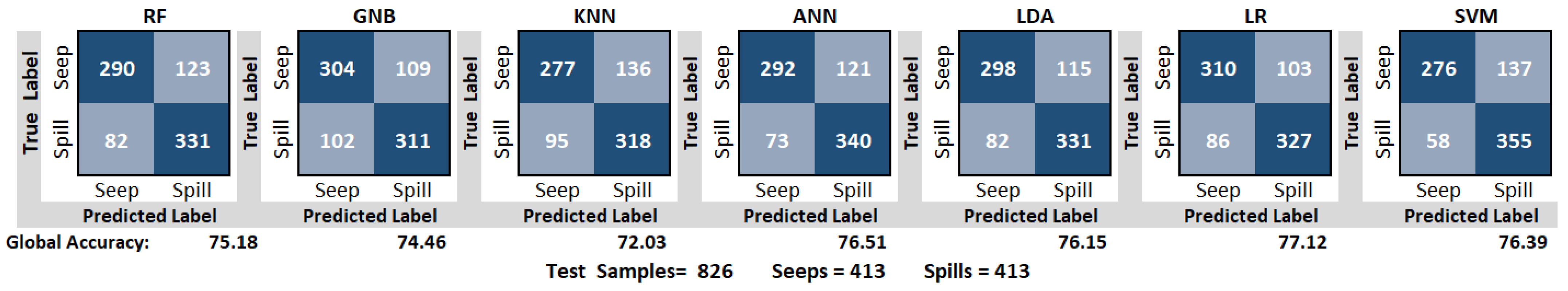
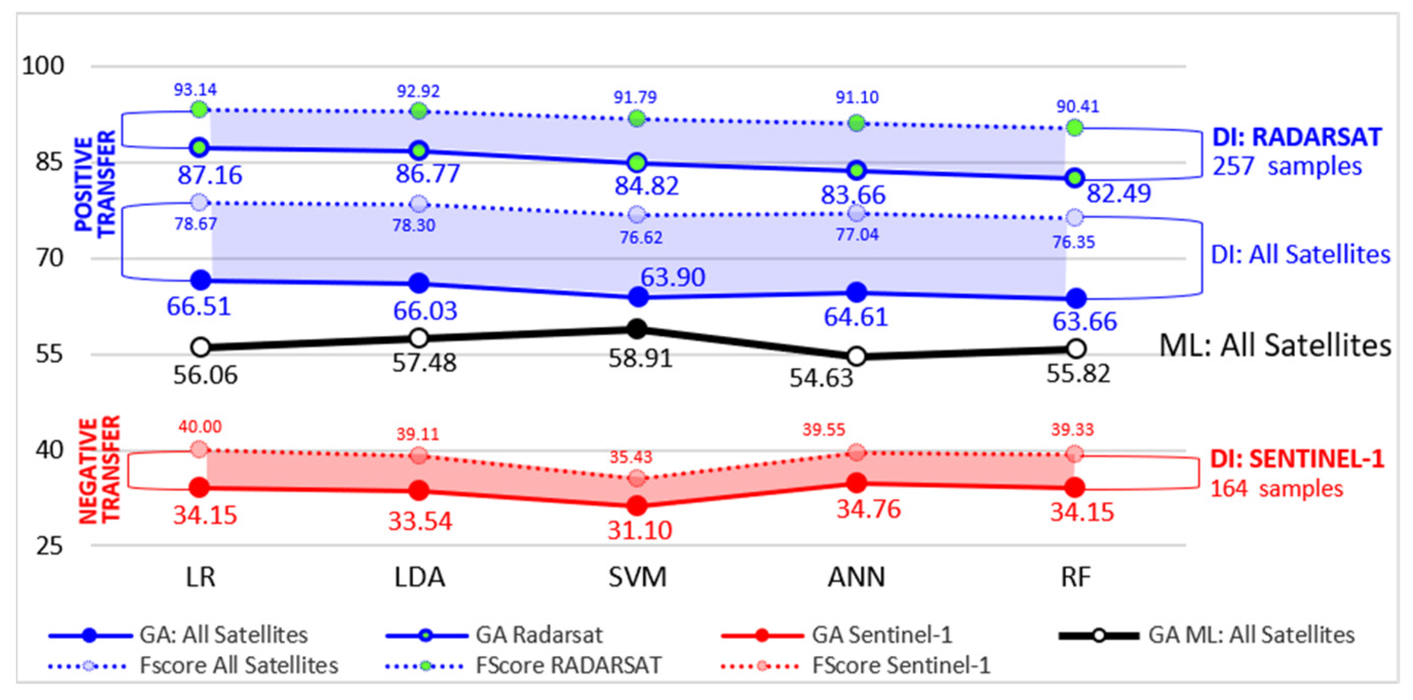
3.2.3. Study Case 3: GoM ⇥ BR

In the third study case, the best predictive functions fS(.) trained, tested, and saved for GoM models employing ANN, RF, SVM, LDA, and LR were domain-adapted fT(.) and applied to predict 421 new samples of natural and anthropic oil slicks detected in BR (Figure 2f,g). In this case, the DS and DT domains are different (DS ≠ DT) not only by using different satellites to detect the samples employed to develop the models (DS: RDS1 and RDS 2) and to infer the OSS (DT: RDS1, RDS2, and SNT1), but also by considering geographic regions completely distinct. Table 7 summarizes the obtained performances comparing traditional ML (Table 7a) with CDS (Table 7b) and DI (Table 7c).
Consistently with previous results, TTL (Table 7b,c) overpasses the traditional ML approach (Table 7a, Figure 11a: red line) for all metrics and methods, returning GA above 63% and F-Score over 76%. Synthesizing, the maximum, minimum, and median values of GA (65.08; 63.42; 64.61), sensitivity (73.41; 71.39; 71.97) and F-Score (77.56; 76.23; 76.90), respectively, employing CDS (Table 7b), as well as GA (66.51; 63.66; 64.61), sensitivity (75.14; 71.39; 72.25) and F-Score (78.67; 76.35; 77.04) performing DI (Table 7c) are higher than all accuracies achieved by traditional ML (Table 7a).
Although the prediction results employing DI (Figure 11a: blue solid line) are nearby to the CDS ones (Figure 11a: blue dashed line), similarly to the GMex ⇥ GAm; evidence endorses the DI with LR as the best prediction function for the OSS inference. Considering the best TL strategy (DI) and ML algorithm (LR), Figure 11b provides the geolocation of the seepage slicks correctly (True Positives: TP) and incorrectly predicted (False Negatives: FN) by the GoM model.
Despite the GoM models trained with all satellites being adapted to predict samples in BR with positive transfers (Figure 11a: solid and dashed blue lines), the gains in terms of performance do not overpass 11% (Table 8b: DifGA), while in the GMex ⇥ GAm case the maximum increment reached 28%. Since the oil slicks detected in the DS domain do not encompass all sets of satellites used to detect in BR the target samples (DT), further analysis was conducted to evaluate how features extracted from different SAR sensors affect the performance of the GoM models in the Brazilian continental margin.
To accomplish this the GoM models were applied to predict samples in BR using the best TL strategy (DI) considering all satellites together (Table 8b), and sorting out RDS (Table 8c) from SNT1 (Table 8d). To maintain a baseline for comparison, the GA(s) and F-Score(s) obtained by all satellites using traditional ML are also inserted (Table 8a; Figure 12: solid black line). The increment or decrement in terms of performances per satellite is highlighted through a subtraction between GA(s) and F-Score(s) obtained by DI, from those obtained by traditional ML (Table 8: DifGA; DifFSc).
It was clear that even employing TL when processing samples from all satellites together, the prediction accuracies in BR were pulled down due to the influence of the SNT1 samples, and do not surpass 66.51% of GA (Table 8b; Figure 12: solid and dashed blue lines with blue markers).
Regarding the RDS samples (Table 8c), the patterns learned from the DS domain effectively improved performances in the DT domain, thus characterizing a substantial positive transfer (Figure 12: solid and dashed blue lines with green markers). The TL was successfully validated returning the higher positive differences obtained by the RDS samples (Table 8c), achieving approximately 31% of maximum increments for GA (Table 8c: DifGA) and nearly 25% for the F-Score (Table 8c: DifFSc). Results are impressive, since even without any prior knowledge of the geometric behaviour of the oil slicks in BR, the GoM model recognized 87% of the seepage slicks detected by RDS sensors using DI and LR.
Conversely, the GoM models trained with RDS samples failed to predict SNT1 samples in BR (Table 8d), provoking negative transfers (Figure 12: red area) with all accuracies (Figure 12: solid and dashed red lines) below those obtained by traditional ML (Figure 12: black line). This ineffective transferability of knowledge to SNT1 samples was evidenced by the meaningful decrements around −28% for GA (Table 8d: DifGA) and nearly −36% for F-Score (Table 8d: DifFSc).
The GoM ⇥ BR application is an example of an aleatoric uncertainty generating an epistemic uncertainty (Section 1.2). In this case, SAR sensors with different configurations in terms of spatial resolution in the DS (RDS: 50m) and DT (SNT1: 10m resized for 20m) domains produced geometric features with statistical distributions so divergent (P(XS) ≠ P(XT)) that it became unfeasible for both DA and TL. The impact of samples detected by SAR sensors with highly diverse spatial resolutions are exemplified, for instance, through oil slicks with equal areas (RDS & SNT1 = 1.52 km2) and similar shapes (RDS: 3.3; SNT1: 4.7) that returned perimeters completely different (RDS: 16.25 km; SNT1: 23.6 km), impacting all derivative geometric features. Consequently, the SNT1 samples in the DT domain were so out-of-distribution that the maximum GA using TL was 35%, below that provided by the traditional ML (59%), thus characterizing a negative transfer (Figure 12: red area).
Fundamentally, the more similar the DS and DT domains are in terms of statistical properties, the better will be the DA, thus the effectiveness of the TL approach. Therefore, the GoM ⇥ BR application suggests that—once employing SAR sensors with similar configurations—it is possible to transfer knowledge from a model trained and tested in a specific geographic region to predict with excellent performance unknown oil slicks located elsewhere, even under distinct meteo-oceanographic conditions.
Despite the fact that both TTL methods presented a successful DA when handled with different domains, it is important to highlight that the DI achieved better performances as seen in Scenarios 2 and 3 (Figure 3). A likely explanation is that the DI predicts one sample at a time, adapting the DT domain to the DS domain, and preserving the original statistical properties of the oil slicks in the DS domain. Conversely, in the joint normalization performed by CDS, both distributions are mutually adapted minimizing the derived effects from data shift and/or drift ((P(XS) ≠ P(XT)), but changing the original pdf(s). It seems that, by predicting sample by sample, the DI avoids the epistemic uncertainty between divergent pdf(s), resulting in better accuracies as shown in Table 6 and Table 7. Therefore, since the DI performed better than the CDS, and the use of all satellites together masks the effect of different SAR sensors, the next Section 3.3 and Section 3.4 prioritized the utilization of DI considering the BR samples per satellite.

3.3. Moving Transfer Learning into the Real World

Moving predictive models into the real world is challenging, not just because it involves the statistical performances of these models (Section 3.1 and Section 3.2), but also a broader architecture designed for operational deployment.
In this context, to minimize interpretability risks implicit in the ML processing chain, the learned results are integrated to define a technical and scientific protocol to operationalize the TL for the OSS prediction. To accomplish this, a comparison (Figure 13a: GoM ⇥ GoM; Figure 13b: GMex ⇥ GAm; Figure 13c: GoM ⇥ BR) among performances reached by the models during the development (Table 3 and Table 4) and application phases (Table 5, Table 6 and Table 8c,d) is important to understand the level of adaptability, responsiveness, and flexibility of the models to learn patterns and generalize them (Figure 13d) across similar and different domains using TL.
Table 9 provides the generalization index (GI) calculated employing CDS (GICDS) and DI (GIDI) for all studied cases: (a) GoM ⇥ GoM; (b) GMex ⇥ GAm; (c) GoM ⇥ BR with RDS and (d) GoM ⇥ BR with SNT1.
When the DS and DT domains are the same (DS = DT), presenting similar statistical properties (P(XS) = P(XT)) as seen in the GoM ⇥ GoM application, the GA(s) and sensitivities (Figure 13a: solid and dashed red lines) are similar to those obtained during the models’ building (Figure 13a: solid and dashed blue lines). In these cases, the OSS inferences are not affected by aleatoric or epistemic uncertainties, and the models’ generalizations are practically null (Table 9a), with GI(s) varying around zero employing CDS (Figure 13d: dashed grey line) or DI (Figure 13d: solid grey line).
As seen in GMex ⇥ GAm and GoM ⇥ BR: RDS, when domains are dissimilar (DS ≠ DT), with different but related pdf(s) (P(XS) ≠ P(XT)), the GA(s) are usually greater (Figure 13b: solid red line; Figure 13c: solid red line with grey markers) than those obtained during the models’ development (Figure 13b: solid blue line; 13c: solid and dashed blue lines). Coherently, the highest GI index of 1.00 (Table 9c) was obtained by the GoM ⇥ BR: RDS application (Figure 13d: solid blue line with green markers) employing DI and LR. Likely, the transferability of geometric properties from the DS to the DT domain is boosted when using the same SAR sensors in both domains, allowing well-fitted data projections, minimizing differences, and improving prediction accuracies. Another good result for a GI of 0.88 (Table 9b) was reached by applying a GMex model over GAm samples using DI and RF (Figure 13d: solid orange line). Probably, the use of similar but different satellites in the DS (RDS2) and DT (RDS1) domains affected this result.
Lastly, when domains are dissimilar (DS ≠ DT) presenting high-divergent statistical properties (P(XS) ≠ P(XT)), as seen in the GoM ⇥ BR: SNT1 application, the GA(s) and sensitivities (Figure 13c: solid and dashed red lines) are significantly lower than those obtained during the models’ building (Figure 13c: solid and dashed blue lines). As aforementioned, aleatoric and epistemic uncertainties affect these predictions making the DA unfeasible, resulting in the worst GI (−1.00) employing CDS and SVM (Table 9d; Figure 13d: dashed red line with blue markers).
Consistently with previous analyses, for all positive transfers the GI(s) are higher than zero, and the DI method generalized better than the CDS. On the contrary, for the negative transfers, CDS and DI returned similar generalization with GI(s) below zero. Employing DI or CDS, the integrated analysis of all measures of effectiveness revealed key configurations for a successful migration of robust and validated applications to an operational environment (OE). Under a TL approach, these configurations are synthesized in Box 2 and comprise three specific behaviours.
Box 2. Protocol to migrate predictive models for OSS identification from developer environments to operational environments employing TL.
Remotesensing 15 01496 i002
Box 2: 1 ⇥ Operational use feasible under restrictions employing ML or TL: protocol useful for same domains (DS = DT), i.e., models developed and applied in the same geographic region, under the same meteo-oceanographic condition, employing the same set of satellites, and using samples with convergent statistical properties. In these cases, the accuracies of the model and the predictions, as well as the ML and TL methods, are similar. The GI(s) are practically null with no significant gain when transferring knowledge. GoM ⇥ GoM configures a typical ML case, which can be operationalized without the need to acquire new samples and retrain the models. These OE(s) will be effective to predict only unknown samples statically equivalent to those used in the model building.
Box 2: 2 ⇥ Operational use feasible employing TL: protocol useful for different but related domains (DS ≠ DT), i.e., models developed and applied in different geographic regions, under distinct meteo-oceanographic conditions, employing satellites with equivalent configurations, and using samples with different but related statistical properties. In these cases, the knowledge learned by the models is positively transferred to infer unknown targets, adapting domains, and improving prediction performances regarding traditional ML. The GI(s) are always positive and such predictive systems (GMex ⇥ GAm; GoM ⇥ BR: RDS) are flexible and adaptable enough to migrate and be deployed into OE(s) without the need of acquiring new samples and retraining the models from scratch.
Box 2: 3 ⇥ Operational use unfeasible: protocol applied to completely different domains (DS ≠ DT), i.e., models developed and applied in different geographic regions, under distinct meteo-oceanographic conditions, employing satellites with incompatible configurations, and using samples with high-divergent statistical distributions. In these cases, it is not possible to adapt domains or to transfer knowledge. The transferability is negative and the prediction accuracies with TL are worse than those obtained with traditional ML. The GI(s) are negative and such predictive systems (GoM ⇥ BR: SNT1) cannot be operationalized, unless new samples are acquired for training new models to recognize geometric patterns extracted from SNT1.
The requirements mapped in this protocol offer explainability and human autonomy, empowering the end-users to make decisions about when and how to apply and migrate predictive models to OE(s). Taking this protocol as a baseline, applications with operational potential were implemented in a proprietary software named GeoqView, making the functionalities available to end-users for testing.

3.4. Operationalizing Predictive Models for OSS Identification: Real-World Case Integrating TL and Inverse Oil Drifting Models

Artificial intelligence is a powerful means of performing analyses that would be humanly impossible, processing simultaneously large data sets and recognizing relationships among geometric patterns of oil slicks detected in different geographic regions. However, when prospecting new exploratory frontiers, automatic systems cannot reproduce the interdisciplinary and highly specialized view of experts when integrating SAR imagery, field data, inverse oil drifting models, and geophysical surveys [4,5]. In this sense, the operational test adopted a broader view, integrating the data-driven and knowledge-driven approaches, using automatic predictions to add value and confidence to the interpreters` analysis.
To accomplish this, remote sensing experts from the oil and gas sector used the GoM ⇥ BR application (DI and LR) implemented in the GeoqView software to infer automatically the OSS of 69 oil slicks carefully interpreted by them as seepage slicks. As synthesized in Figure 14, from 69 interpreted samples 54 (78%) were correctly predicted as seepage slicks (Figure 14a blue points; 14b) and 15 (22%) were incorrectly recognized as oil spills (Figure 14a red points; 17b). Coherently (Figure 14b), 76% of the correctly predicted samples were detected by RDS sensors, the same used for building the GoM model, while 87% of the incorrectly predicted samples were detected by SNT1, a satellite not considered during the training. Remarkably, considering only RDS samples, 41 out of 43 seepage slicks were correctly inferred achieving 95% of global accuracy, whereas for SNT1 samples only 13 (50%) from 26 seepage slicks were correctly predicted.
Sequentially, an inverse oil drifting model (IODM) was used to estimate, for each seepage slick, the inverse oil slick trajectory from the sea surface to the ocean bottom (Figure 14a blue lines) [23,24]. When three or more seepage slicks converge to the same seafloor area, a detailed investigation is conducted for seeking the geologic structures and faults probably connected with active petroleum systems [23,24].
In this real-operational test, out of the 17 convergence regions (CR) identified by IODM, 5 had all the interpreted seepage slicks (100%) confirmed by the automatic predictions, and 6 returned prediction accuracies were greater than or equal to 75% (Figure 14c). A map ranking the CR per the number of slicks interpreted as seepage slicks and confirmed by the automatic predictions represents key information to guide decision-making, pointing out priority regions to concentrate investments during the exploratory phase.

4. Discussion

Comparing the obtained results with past research on the topic is difficult, since the majority of published papers are dedicated to discriminate oil spills from look-alikes, or to extract dark spots from SAR sensors [25,26,27,28,29,30,31,32,33,34,35,36,37,38,39,40]. Part of available research used SAR data to discover, map and catalogue sources of seepage slicks around the globe, extracting information regarding shape, dimensions, spatial recurrence, and other characteristics [2,3,4,5,44]. However, discriminating seepage slicks from oil spills using SAR sensors and ML is a new and promising research area.
Previous studies [42,87,88] carried out with oil slicks carried out detection by using RDS sensors, integrating radiometric with geometric features, and employing LDA to discriminate seepage slicks from oil spills; a maximum accuracy of 70% was achieved. These studies developed and applied the classification models to infer samples acquired in the same geographic region and detected with the same SAR sensor, characterizing a traditional ML approach.
The present research not only applied a traditional ML approach in scenario 1, but also went further to test—in an unprecedented way—TL for transferring knowledge from validated models for inferring the OSS of new samples detected in different geographic regions (scenarios 2 and 3). Other novelty aspects are: (i) the employment of only geometric features to discriminate seepage slicks from oil spills, considering a higher diversity of attributes when compared with previous studies [35]; (ii) the creation of a new metric named the Generalization Index to evaluate the relative transferability of developed predictive models when applied over distinct geographic regions; (iii) the evaluation of the effects provoked by different SAR sensors (RDS and SNT1), comprising different configurations in terms of image beam modes, noise equivalent sigma zero, and spatial resolutions. Results were promising since, besides corroboration with ML and TL theory, they provided concrete evidence of the feasibility to adapt different domains when employing TL in an operational way. Figure 15 illustrates a comparison between the maximum global accuracy achieved by previous works with the results obtained in this research project.
The promising results reflect the technical and ethical guidelines [57,58,59] adopted to develop, apply, and deploy predictive models for OSS identification. The end-user’s co-assessment inserted the stakeholders’ perspective in all phases of the project which allowed the development of transparent, robust, and fair models validated through several measures of effectiveness (Section 2.2). The HOL mechanism guaranteed the transparency of results through several measures of effectiveness, aggregating the end-user’s expertise to oversee and test the systems’ development, deployment, and operational use. Moreover, the audits undertaken by experts from the oil and gas industry ensured the robustness and quality of the dataset, making possible the development of trustworthy predictive models. Sets of balanced and validated oil slicks (Figure 2) as input ensured fairness, avoiding biased inferences, improving the discriminative potential of the models, and boosting the TL across different domains.

5. Conclusions

The employment of controlled feature spaces (XS) as input in the DS domain allowed the development of two predictive models well-trained to recognize representative geometric patterns of natural and anthropic oil slicks: (1) the GMex model, achieving a test accuracy of 77% using RDS2; and (2) the GoM model, attaining 75% by employing RDS1 and RDS2.
In an unprecedented way, these models were successfully applied to predict the OSS in different DT domains using TL. When domains are the same (DS = DT), with equivalent statistical properties (GoM ⇥ GoM), the models’ transferability and generalization are practically null, and the maximum prediction performances are identical using TL or ML (75.93%). In such cases, the operational deployment is viable without the need to adapt domains or retrain the models with newly validated samples. However, when domains are different (DS ≠ DT), it is discernible circumstances in which the knowledge learned by the model is positively transferred to unknown samples, adapting domains and improving prediction performances (GMex ⇥ GAm and GoM ⇥ BR: RDS), as well as extreme situations of negative transfer (GoM ⇥ BR: SNT1), where it is not possible neither to adapt domains nor to transfer knowledge due to the high-data-divergence.
Even without any prior knowledge about the geometry and behaviour of the oil slicks, in the positive transfers the maximum global accuracies using TL (GAGMex ⇥ GAm = 80%; GAGoM ⇥ BR: RDS = 87%) were much higher than those provided by usual ML (GAGMex ⇥ GAm = 52%; GAGoM ⇥ BR: RDS = 59%). Consequently, the positive generalizations (GIGoM ⇥ BR: RDS = 1.00; GIGMex ⇥ GAm = 0.83) for the first time ever showed the adaptability and flexibility of these well-trained models to learn and transfer geometric patterns to make inferences in different domains. These outcomes suggest the existence of an explicit and/or implicit relationship between the geometric properties of oil slicks detected in distinct geographic regions, making it unnecessary to acquire new labelled samples, or to retrain the models from scratch.
Nevertheless, the transferability and generalization capacity of predictive models are limited when the SAR sensors used in the DS and DT domains have different configurations, characterizing a negative transfer. Since the domain adaptation was unfeasible, the operational use of the GoM ⇥ BR: SNT1 application is not recommended. Its maximum accuracy using TL (GAGoM ⇥ BR: SNT1 = 35%) was lower than that provided by traditional ML (GAGoM ⇥ BR = 59%), and its generalization was negative (GIGoM ⇥ BR: SNT1 = −1.00).
Results revealed not only the adaptability and responsiveness of these models to operate in different scenarios with outstanding performances, but also their limitations grounding the creation of an unprecedented protocol for operational deployment of TL aiming at OSS identification. This protocol complies with the HIC mechanism, making the potential and limitation of the TL methods human-interpretable, and reinforcing human autonomy by boosting the confidence of end-users to decide when and how to apply the automatic inferences.
Despite the uncertainties embedded in any statistical inference process, this protocol was validated by a real-operational test (GoM ⇥ BR) confirming 95% of the seepage slicks classified by the interpreters when using same satellites (RDS), and only 50% when using different satellites (SNT1).
Therefore, this RD&I project for the first-time remarkably evidenced that it is fully possible to operationalize predictive systems using TL to identify the OSS of unknown samples acquired in different geographic regions, under distinct meteo-oceanographic contexts, using satellites with compatible configurations, and considering only geometric properties. The integration of data-driven and knowledge-driven approaches are powerful and have shown how AI-based systems can be used not to replace, but to add confidence to the experts’ interpretation, strengthening their technical reports and decision-making.
Beyond the reported scientific benefits, important economic and environmental impacts were achieved by the project outcomes. The main economic impact offered by TL is the concrete possibility to save time and budget with the collection, validation, and labelling of new samples, as well as with the re-training of new models. Furthermore, since there is no similar software available in the market, an expert system like that, architected to operate within corporative environments and to process confidential data sensitive for the oil and gas industry, represents a profitable investment with a guaranteed return.
From the exploratory point of view, oil and gas companies can use the convergence regions joint with seepage slicks automatically confirmed as hot-spots to aggregate value to the blocks during bidding rounds. Automatic predictions can also be strategically employed to create a ranking of these regions per importance order, supporting the exploratory activities planning, thus optimizing time, costs, human resources, and infrastructure. The possibility of minimizing the confusion between seepage slicks and oil spills represents a value-added product that can contribute to reducing geologic risks when seeking active petroleum systems associated with present-day oil generation and migration in new exploratory frontiers.
Additionally, in offshore oil exploration and production fields, where seepage slicks and oil spills can simultaneously occur, well-trained models to discriminate natural from anthropic events using SAR sensors can protect the oil industry against penalties for pollution events. On the other hand, the prompt identification of an oil spill can speed up the response actions to clean-up and protect sensitive areas against oil pollution.
Lastly, as unreported oil slicks are considered in new cycles of training and testing, the predictive models increasingly become more effective in recognizing known and novel geometric patterns, transferring knowledge between domains, thus improving their generalization and prediction accuracies. The continuous increment of the database with newly validated oil slick samples constitutes a future priority for the project, embracing different regions of interest for the petroleum industry and other SAR sensors. Another promising future perspective is testing further DA methods, such as dimensionality reduction, aiming to optimize the TL to different DT domains, hence boosting the models’ generalization capacity.

Author Contributions

Conceptualization, P.C.G., F.F.d.A.P., Í.d.O.M., F.P.d.M. and G.M.A.S.; methodology, P.C.G., F.F.d.A.P., Í.d.O.M., C.H.B., M.F.M., F.P.d.M. and G.M.A.S.; software, F.F.d.A.P., Í.d.O.M., P.C.G., S.B.T. and M.F.M.; validation, P.C.G., F.F.d.A.P., Í.d.O.M., F.P.d.M., G.M.A.S. and C.H.B.; formal analysis, P.C.G. and F.F.d.A.P.; investigation, P.C.G., F.F.d.A.P., Í.d.O.M., F.P.d.M. and G.M.A.S.; resources F.P.d.M., G.M.A.S. and Í.d.O.M.; data curation, F.P.d.M., G.M.A.S., C.H.B. and M.F.M..; writing—original draft preparation, P.C.G.; writing—review and editing, F.P.d.M., F.F.d.A.P., Í.d.O.M. and S.B.T.; visualization, P.C.G.; supervision, Í.d.O.M., F.P.d.M. and G.M.A.S.; project administration, F.P.d.M., G.M.A.S. and Í.d.O.M.; funding acquisition F.P.d.M., G.M.A.S. and Í.d.O.M. All authors have read and agreed to the published version of the manuscript.

Funding

Petroleo Brasileiro S.A. (Petrobras) funded this study in the context of the Cooperation Agreement 2017/00777-6 with the Pontifical Catholic University at Rio de Janeiro (PUC-Rio).

Data Availability Statement

Not applicable.

Acknowledgments

The authors are grateful to Petróleo Brasileiro S.A. (Petrobras) for providing funds for this project. The authors would also like to acknowledge the Software Engineering Lab (LES) of PUC-Rio, for providing all in-house software used to process the dataset.

Conflicts of Interest

The authors declare no conflict of interest.

References

  1. Committee on Oil in the Sea; Divisions of Earth and Life Studies and Transportation Research Board, National Research Council. Oil in the Sea III: Inputs, Fates, and Effects; National Academies Press: Washington, DC, USA, 2003; ISBN 978-0-309-08438-3. [Google Scholar] [CrossRef]
  2. MacDonald, I.R.; Garcia-Pineda, O.; Beet, A.; Asl, S.D.; Feng, L.; Graettinger, G.; French-McCay, D.; Holmes, J.; Hu, C.; Huffer, F.; et al. Natural and unnatural oil slicks in the Gulf of Mexico. J. Geophys. Res. Oceans 2015, 120, 8364–8380. [Google Scholar] [CrossRef] [PubMed]
  3. Garcia-Pineda, O.; MacDonald, I.; Silva, M.; Shedd, W.; Asl, S.D.; Schumaker, B. Transience and persistence of natural hydrocarbon seepage in Mississippi Canyon, Gulf of Mexico. Deep-Sea Res. Part II: Topical Stud. In Oceanogaphyr. 2016, 129, 119–129. [Google Scholar] [CrossRef] [Green Version]
  4. Dembicki, H., Jr. Reducing the risk of finding a working petroleum system using SAR imaging, sea surface slick sampling, and geophysical seafloor characterization: An example from the eastern Black Sea basin, offshore Georgia. Mar. Pet. Geol. 2020, 115, 104276. [Google Scholar] [CrossRef]
  5. O’Reilly, C.; Silva, M.; Daneshgar, A.S.; Meurer, W.P.; MacDonald, I.R. Distribution, Magnitude, and Variability of Natural Oil Seeps in the Gulf of Mexico. Remote Sens. 2022, 14, 3150. [Google Scholar] [CrossRef]
  6. Alpers, W.; Espedal, H.A. Chapter 11: Oils and surfactants. In Synthetic Aperture Radar Marine User’s Manual; Jackson, C.R., Apel, J.R., Eds.; U.S. Department of Commerce, National Oceanic and Atmospheric Administration: Washington, DC, USA, 2004; pp. 263–275. [Google Scholar]
  7. Leifer, I.; Lehr, B.; Simecek-Beatty, D.; Bradley, E.; Clark, R.; Dennison, P.; Hu, Y.; Matheson, S.; Jones, C.; Holt, B.; et al. State of the art satellite and airborne marine oil spill remote sensing: Application to the BP Deepwater Horizon oil spill. Remote Sens. Environ. 2012, 124, 185–209. [Google Scholar] [CrossRef] [Green Version]
  8. Dong, Y.; Liu, Y.; Hu, C.; MacDonald, I.R.; Lu, Y. Chronic oiling in global oceans. Science 2022, 376, 1300–1304. [Google Scholar] [CrossRef]
  9. International Tanker Owners Pollution Federation Limited (ITOPF). Handbook: Promoting Effective Spill Response. 2022; pp. 1–60. Available online: https://www.itopf.org/fileadmin/uploads/itopf/data/Documents/Company_Lit/ITOPF_Handbook22_web.pdf (accessed on 5 December 2022).
  10. ESA Publication: Earth Observation for Sustainable Development Goals—Compendium of Guidance on Earth Observation to Support the Targets and Indicators of the SDG. ESA Contract No. 4000123494/18/I-NB. 2020. Available online: https://eo4society.esa.int/wp-content/uploads/2021/01/EO_Compendium-for-SDGs.pdf (accessed on 10 November 2022).
  11. Persello, C.; Wegner, J.D.; Hansch, R.; Tuia, D.; Ghamisi, P.; Koeva, M.; Camps-Valls, G. Deep Learning and Earth Observation to Support the Sustainable Development Goals: Current approaches, open challenges, and future opportunities. IEEE Geosci. Remote Sens. Mag. 2022, 10, 172–200. [Google Scholar] [CrossRef]
  12. Johnson, C.D.; Ruiter, J.M. Publication developed by International Space University and University of South Australia. In Final Report Southern Hemisphere Space Studies Program: Space 2030: Space for the Future, Space for All; International Space University: Illkirch-Graffenstaden, France, 2019. [Google Scholar]
  13. API (American Petroleum Institute). Remote Sensing in Support of Oil Spill Response: Planning Guidance; Technical Report No. 1144; American Petroleum Institute: Washington, DC, USA, 2013. [Google Scholar]
  14. IPIECA (International Petroleum Industry Environmental Conservation Association). An Assessment of Surface Surveillance Capabilities for Oil Spill Response Using Satellite Remote Sensing; Technical Report PIL-4000–35-TR-1.0; International Petroleum Industry Environmental Conservation Association: London, UK, 2014. [Google Scholar]
  15. Fingas, M.; Brown, C.E. A Review of Oil Spill Remote Sensing. Sensors 2018, 18, 91. [Google Scholar] [CrossRef] [Green Version]
  16. Alpers, W.; Hühnerfuss, H. The damping of ocean waves by surface films: A new look at an old problem. J. Geophys. Res. Space Phys. 1989, 94, 6251–6265. [Google Scholar] [CrossRef]
  17. Holt, B. Chapter 02: SAR Imaging of the Ocean Surface. In Synthetic Aperture Radar Marine User’s Manual; Jackson, C.R., Appl, J.R., Eds.; U.S. Department of Commerce, National Oceanic and Atmospheric Administration: Washington DC, USA, 2004; pp. 263–275. [Google Scholar]
  18. Brekke, C.; Solberg, A.H.S. Oil spill detection by satellite remote sensing. Remote Sens. Environ. 2005, 95, 1–13. [Google Scholar] [CrossRef]
  19. Richards, J.A. Remote Sensing with Imaging Radar. In Aperture Antennas for Millimeter and Sub-Millimeter Wave Applications; Springer: Berlin/Heidelberg, Germany, 2009. [Google Scholar]
  20. Caruso, M.J.; Migliaccio, M.; Hargrove, J.T.; Garcia-Pineda, O.; Graber, H.C. Oil spills and slicks imaged by synthetic aperture radar. Oceanography 2013, 26, 112–123. [Google Scholar] [CrossRef] [Green Version]
  21. Alpers, W.; Holt, B.; Zeng, K. Oil spill detection by imaging radars: Challenges and pitfalls. Remote Sens. Environ. 2017, 201, 133–147. [Google Scholar] [CrossRef]
  22. Matias, I.O.; Genovez, P.C.; Torres, S.B.; Araújo, F.F.P.; Oliveira, A.J.S.; Miranda, F.P.; Silva, G.M.S. Improved Classification Models to Distinguish Natural from Anthropic Oil Slicks in the Gulf of Mexico: Seasonality and Radarsat-2 Beam Mode Effects under a Machine Learning Approach. Remote Sens. 2021, 13, 4568. [Google Scholar] [CrossRef]
  23. Mano, M.; Beisl, C.H.; Soares, C. Oil Seeps on the Seafloor of Perdido, Mexico. In Proceedings of the AAPG 2016 International Convention and Exhibition, Cancun, Mexico, 6–9 September 2016. [Google Scholar]
  24. Mano, M.; Beisl, C.H.; Landau, L. Identifying Oil Seep Areas at Seafloor Using Oil Inverse Modeling. In Proceedings of the Article #90135©2011 AAPG International Conference and Exhibition, Milan, Italy, 23–26 October 2011. [Google Scholar]
  25. Bjerde, K.; Solberg, A.; Solberg, R. Oil spill detection in SAR imagery. Int. Geosci. Remote Sens. Symp. 2002, 3, 943–945. [Google Scholar] [CrossRef]
  26. Solberg, A.H.; Storvik, G.; Solberg, R.; Volden, E. Automatic Detection of Oil Spills in ERS SAR Images. IEEE Trans. Geosci. Remote Sens. 1999, 37, 1916–1924, Publisher Item Identifier S 0196-2892(99)03483-X. [Google Scholar] [CrossRef] [Green Version]
  27. Solberg, R.; Theophilopoulos, N.A. Envisys—A solution for automatic oil spill detection in the Mediterranean. In Proceedings of the 4th Thematic Conference on Remote Sensing for Marine and Coastal, Ann Arbor, MI, USA, 1 June 1997; Environmental Research Institute of Michigan: Ann Arbor, MI, USA, 1997; pp. 3–12. [Google Scholar]
  28. Solberg, A.H.S.; Dokken, S.T.; Solberg, R. Automatic detection of oil spills in Envisat, Radarsat and ERS SAR images. In Proceedings of the International Geoscience and Remote Sensing Symposium, Toulouse, France, 21–25 July 2003; Volume 4. [Google Scholar] [CrossRef]
  29. Solberg, A.; Clayton, P.; Indregard, M. D2–Report on Benchmarking Oil Spill Recognition Approaches and Best Practice. Kongsberg Satellite Services–Norway Archive No.: 04-10225-A-Doc, Issue/Revision, 2.1. 2005. Available online: www.ksat.no (accessed on 29 November 2006).
  30. Kubat, M.; Holte, C.; Matwin, S. Machine learning for detection of oil spills in satellite Radar images. Mach. Learn. 1998, 30, 195–215. [Google Scholar] [CrossRef] [Green Version]
  31. Fiscella, B.; Giancaspro, A.; Nirchio, F.; Pavese, P.; Trivero, P. Oil spill detection using marine SAR images. Int. J. Remote. Sens. 2000, 21, 3561–3566. [Google Scholar] [CrossRef]
  32. Mera, D.; Cotos, J.M.; Varela-Pet, J.; Rodríguez, P.G.; Caro, A. Automatic decision support system based on SAR data for oil spill detection. Comput. Geosci. 2014, 72, 184–191. [Google Scholar] [CrossRef] [Green Version]
  33. Al-Ruzouq, R.; Gibril, M.B.A.; Shanableh, A.; Kais, A.; Hamed, O.; Al-Mansoori, S.; Khalil, M.A. Sensors, Features, and Machine Learning for Oil Spill Detection and Monitoring: A Review. Remote Sens. 2020, 12, 3338. [Google Scholar] [CrossRef]
  34. Topouzelis, K.; Psyllos, A. Oil spill feature selection and classification using decision tree forest on SAR image data. J. Photogramm. Remote Sens. 2012, 68, 135–143. [Google Scholar] [CrossRef]
  35. Genovez, P.C.; Ebecken, N.F.F.; Freitas, C.C.; Bentz, C.M.; Freitas, R.M. Intelligent hybrid system for dark spot detection using SAR data. Expert Syst. Appl. 2017, 81, 384–397. [Google Scholar] [CrossRef]
  36. Mera, D.; Bolon-Canedo, V.; Cotos, J.M.; Alonso-Betanzos, A. On the use of feature selection to improve the detection of sea oil spills in SAR images. Comput. Geosci. 2017, 100, 166–178. [Google Scholar] [CrossRef]
  37. Keramitsoglou, I.; Cartalis, C.; Kiranoudis, C. Automatic identification of oil spills on satellite images. Environ. Model. Softw. 2006, 21, 640–652. [Google Scholar] [CrossRef]
  38. Karathanassi, V.; Topouzelis, K.; Pavlakis, P.; Rokos, D. An object-oriented methodology to detect oil spills. Int. J. Remote Sens. 2006, 27, 5235–5251. [Google Scholar] [CrossRef]
  39. Topouzelis, K.N. Oil spill detection by SAR images: Dark formation detection, feature extraction and classification algorithms. Sensors 2008, 8, 6642–6659. [Google Scholar] [CrossRef] [PubMed] [Green Version]
  40. Migliaccio, M.; Nunziata, F.; Buono, A. SAR polarimetry for sea oil slick observation. Int. J. Remote Sens. 2015, 36, 3243–3273. [Google Scholar] [CrossRef] [Green Version]
  41. Miranda, F.P.; Marmol, A.M.Q.; Pedroso, E.C.; Beisl, C.H.; Welgan, P.; Morales, L.M. Analysis of RADARSAT-1 data for offshore monitoring activities in the Cantarell Complex, Gulf of Mexico, using the unsupervised semivariogram textural classifier (USTC). Can. J. Remote Sens. 2004, 30, 424. [Google Scholar] [CrossRef]
  42. Carvalho, G.D.A.; Minnett, P.J.; Paes, E.T.; Miranda, F.P.; Landau, L. Oil-Slick Category Discrimination (Seeps vs. Spills): A Linear Discriminant Analysis Using RADARSAT-2 Backscatter Coefficients (σ°, β°, and γ°) in Campeche Bay (Gulf of Mexico). Remote Sens. 2019, 11, 1652. [Google Scholar] [CrossRef] [Green Version]
  43. Miranda, F.P.; Silva, G.M.A.; Matias, I.O.; Genovez, P.C.; Torres, S.B.; Ponte, F.F.A.; Oliveira, A.J.S.; Nasser, R.B.; Robichez, G. Machine learning to distinguish natural and anthropic oil slicks: Classification model and the Radarsat-2 beam mode effects. In Proceedings of the Rio Oil & Gas Expo and Conference, Rio de Janeiro, Brazil, 21–24 September 2020. [Google Scholar] [CrossRef]
  44. Miranda, F.P.; Silva, G.M.A.; Matias, I.O.; Genovez, P.C.; Torres, S.B.; Ponte, F.F.A.; Oliveira, A.J.S.; Beisl, C.H. Geometric Pattern Recognition Using Machine Learning: Predictive Models to Distinguish Natural from Anthropic Oil Slicks in The Gulf of Mexico. In Proceedings of the Rio Oil & Gas Expo and Conference, Rio de Janeiro, Brazil, 26–29 September 2022. [Google Scholar] [CrossRef]
  45. Pan, S.J.; Yang, Q. A Survey on Transfer Learning. IEEE Trans. Knowl. Data Eng. 2009, 22, 1345–1359. [Google Scholar] [CrossRef]
  46. Kouw, W.M.; Loog, M. Technical Report: An Introduction to Domain Adaptation and Transfer Learning; Cornell University: Ithaca, NY, USA, 2019; pp. 1–41. [Google Scholar] [CrossRef]
  47. Daume, H., III; Marcu, D. Domain Adaptation for Statistical Classifiers. J. Artif. Intell. Res. 2006, 26, 101–126. [Google Scholar] [CrossRef]
  48. Uguroglu, S.; Carbonell, J. Feature Selection for Transfer Learning. In Lecture Notes in Computer Science, Proceedings of the ECML PKDD: Joint European Conference on Machine Learning and Knowledge Discovery in Databases, V III, Athens, Greece, 5–9 September 2011; Springer: Berlin/Heidelberg, Germany, 2011; pp. 430–442. [Google Scholar]
  49. Crosby, C. Operationalizing Artificial Intelligence for Algorithmic Warfare. Military Reiew. 2020, 42–51. [Google Scholar]
  50. Pan, S.J.; Kwok, J.T.; Yang, Q. Transfer Learning via Dimensionality Reduction. In Proceedings of the Twenty-Third AAAI Conference on Artificial Intelligence, Chicago, IL, USA, 13–17 July 2008; pp. 677–682. Available online: https://www.aaai.org/Papers/AAAI/2008/AAAI08-108.pdf (accessed on 1 March 2022).
  51. Ando, R.K.; Zhang, T. A Framework for Learning Predictive Structures from Multiple Tasks and Unlabeled Data. J. Mach. Learn. Res. 2005, 6, 1817–1853. [Google Scholar]
  52. Arnold, A.; Nallapati, R.; Cohen, W.W. A Comparative Study of Methods for Transductive Transfer Learning. In Proceedings of the Seventh IEEE International Conference on Data Mining Workshops, Omaha, NE, USA, 28–31 October 2007; pp. 77–82. Available online: https://ieeexplore.ieee.org/document/4476649 (accessed on 1 March 2022). [CrossRef]
  53. Ben-David, S.; Blitzer, J.; Crammer, K.; Pereira, F. Analysis of representations for domain adaptation. Conference: Advances in Neural Information Processing Systems 19. In Proceedings of the Twentieth Annual Conference on Neural Information Processing Systems, Vancouver, BC, Canada, 4–7 December 2006. [Google Scholar]
  54. Raina, R.; Ng, A.Y.; Koller, D. Constructing Informative Priors using Transfer Learning. In Proceedings of the 23rd International Conference on Machine Learning, Pittsburgh, PA, USA, 25–29 June 2006; pp. 713–720. [Google Scholar]
  55. Quinonero-Candela, J.; Sugiyama, M.; Schwaighofer, A.; Lawrence, N. Dataset Shift in Machine Learning; Massachusetts Institute of Technology Press: Cambridge, MA, USA, 2009; ISBN 978-0-262-17005-5. [Google Scholar]
  56. Barnett, M.R. Tools for Multivariate Geostatistical Modeling. In Guidebook Series; Published by the Center for Computational Geostatistics; University of Alberta: Edmonton, AB, Canada, 2021; Volume 13, pp. 1–107. Available online: http://www.uofaweb.ualberta.ca/ccg/ (accessed on 1 May 2022).
  57. European Commission Publication Developed by the High-Level Expert Group on Artificial Intelligence. Ethics Guidelines for Trustworthy AI. 2019; pp. 1–41. Available online: https://digital-strategy.ec.europa.eu/en/library/ethics-guidelines-trustworthy-ai (accessed on 10 November 2022).
  58. European Commission Publication Developed by the High-Level Expert Group on Artificial Intelligence. The Assessment List for Trustworthy Artificial Intelligence (ALTAI) for Self-Assessment. 2020; pp. 1–34. ISBN 978-92-76-20008-6. Available online: https://digital-strategy.ec.europa.eu/en/library/assessment-list-trustworthy-artificial-intelligence-altai-self-assessment (accessed on 10 November 2022). [CrossRef]
  59. European Commission Publication: DG Research & Innovation RTD.03.001-Research Ethics and Integrity Sector. Ethics by Design and Ethics of Use Approaches for Artificial Intelligence. 2021; pp. 1–28. Available online: https://ec.europa.eu/info/funding-tenders/opportunities/docs/2021-2027/horizon/guidance/ethics-by-design-and-ethics-of-use-approaches-for-artificial-intelligence_he_en.pdf (accessed on 10 November 2022).
  60. Baatz, M.; Benz, U.; Dehghani, S. User Guide 3: ECognition Object-Oriented Image Analysis; Definiens Imaging: München, Germany, 2003. [Google Scholar]
  61. Barnes, R.; Solomon, J. Gerrymandering and compactness: Implementation flexibility and abuse. Political Anal. 2021, 29, 448–466. [Google Scholar] [CrossRef]
  62. Topouzelis, K.; Stathakis, D.; Karathanassi, V. Investigation of genetic algorithms contribution to feature selection for oil spill detection. Int. J. Remote Sens. 2009, 30, 611–625. [Google Scholar] [CrossRef]
  63. Stathakis, D.; Topouzelis, K.; Karathanassi, V. Large-scale feature selection using evolved neural networks. In Proceedings of the SPIE the International Society for Optical Engineering, Image and Signal Processing for Remote Sensing XII, Stockholm, Sweden, 11–14 September 2006; Volume 6365, pp. 1–9. [Google Scholar] [CrossRef]
  64. Bentz, C.; Ebecken, N.F.; Politano, A.T. Automatic recognition of coastal and oceanic environmental events with orbital radars. IEEE Int. Geosci. Remote Sens. Symp. 2007, 1, 914–916. [Google Scholar] [CrossRef]
  65. Abiodun, O.I.; Kiru, M.U.; Jantan, A.; Omolara, A.E.; Dada, K.V.; Umar, A.M.; Gana, U. Comprehensive Review of Artificial Neural Network Applications to Pattern Recognition. IEEE Access 2019, 7, 158820–158846. [Google Scholar] [CrossRef]
  66. Belgiu, M.; Dragut, L. Random forest in remote sensing: A review of applications and future directions. ISPRS J. Photogramm. Remote Sens. 2016, 114, 24–31. [Google Scholar] [CrossRef]
  67. Hemachandran, K.; Tayal, S.; George, P.M.; Singla, P.; Kose, U. Bayesian Reasoning and Gaussian Processes for Machine Learning Applications; Imprint Chapman and Hall/CRC: New York, NY, USA, 2022; ISBN 9781003164265. [Google Scholar] [CrossRef]
  68. Mai, Q. A review of discriminant analysis. in high dimensions. Wiley Periodicals, Inc. WIREs Comput. Stat. 2013. [Google Scholar] [CrossRef]
  69. Mountrakis, G.; Im, J.; Ogole, C. Support vector machines in remote sensing: A review. ISPRS J. Photogramm. Remote Sens. 2011, 66, 247–259. [Google Scholar] [CrossRef]
  70. Marsland, S. Machine Learning an Algorithmic Perspective. In Chapman & Hall/CRC Machine Learning & Pattern Recognition Series, 2nd ed.; CRC Press: Boca Raton, FL, USA; Taylor & Francis Group: Abingdon, UK, 2015; ISBN 13 978-1-4665-8333. [Google Scholar]
  71. Dhanabal, S.; Chandramathi, S. A Review of various k-Nearest Neighbor Query Processing Techniques. Int. J. Comput. Appl. 2011, 31, 14–22. [Google Scholar]
  72. Lampropoulos, A.S.; Tsihrintzis, G.A. Machine Learning Paradigms: Applications in Recommender Systems; Springer International Publishing: Cham, Switzerland, 2015; p. 92. [Google Scholar] [CrossRef]
  73. Murphy, K.P. Machine Learning: A Probabilistic Perspective; Massachusetts Institute of Technology MIT Press: Cambridge, MA, USA; London, UK, 2012; ISBN 978-0-262-01802-9. [Google Scholar]
  74. Lu, D.; Weng, Q. A survey of image classification methods and techniques for improving classification performance. Int. J. Remote Sens. 2007, 28, 823–870. [Google Scholar] [CrossRef]
  75. Maxwell, A.E.; Warner, T.A.; Fang, F. Implementation of machine-learning classification in remote sensing: An applied review. Int. J. Remote Sens. 2018, 39, 2784–2817. [Google Scholar] [CrossRef] [Green Version]
  76. Del Frate, F.; Petrocchi, A.; Lichtenegger, J.; Calabresi, G. Neural networks for oil spill detection using ERS-SAR Data. IEEE Trans. Geosci. Remote Sens. 2000, 38, 2282–2287, Publisher Item Identifier S 0196-2892(00)08910-5. [Google Scholar] [CrossRef] [Green Version]
  77. Topouzelis, K.; Karathanassi, V.; Pavlakis, P.; Rokos, D. Detection and discrimination between oil spills and look-alike phenomena through neural networks. ISPRS J. Photogramm. Remote Sens. 2007, 62, 264–270. [Google Scholar] [CrossRef]
  78. Xu, L.; Li, J.; Brenning, A. A comparative study of different classification techniques for marine oil spill identification using RADARSAT-1 imagery. Remote Sens. Environ. 2014, 141, 14–23. [Google Scholar] [CrossRef]
  79. Cao, Y.; Linlin Xu, L.; Clausi, D. Exploring the Potential of Active Learning for Automatic Identification of Marine Oil Spills Using 10-Year (2004–2013) RADARSAT Data. Remote Sens. 2017, 9, 1041. [Google Scholar] [CrossRef] [Green Version]
  80. Zhang, Y.; Li, Y.; Liang, X.S.; Tsou, J. Comparison of Oil Spill Classifications Using Fully and Compact Polarimetric SAR Images. Appl. Sci. 2017, 7, 193. [Google Scholar] [CrossRef] [Green Version]
  81. Liu, P.; Li, Y.; Liu, B.; Chen, P.; Xu, J. Semi-Automatic Oil Spill Detection on X-Band Marine Radar Images Using Texture Analysis, Machine Learning, and Adaptive Thresholding. Remote Sens. 2019, 11, 756. [Google Scholar] [CrossRef] [Green Version]
  82. Mercier, G. Partially Supervised Oil-Slick Detection by SAR Imagery Using Kernel Expansion. IEEE Trans. Geosci. Remote Sens. 2006, 44, 2839–2846. [Google Scholar] [CrossRef]
  83. Azamathulla, H.M.; Wu, F.C. Support Vector Machine approach for longitudinal dispersion coefficients in natural streams. Appl. Soft Comput. 2011, 11, 2902–2905. [Google Scholar] [CrossRef]
  84. Azamathulla, H.M.; Ghani, A.A.; Chang, C.K.; Hasan, Z.A.; Zakaria, N.A. Machine learning approach to predict sediment load–a case study. Clean–Soil Air Water 2010, 38, 969–976. [Google Scholar] [CrossRef]
  85. Mather, P.M.; Koch, M. Chapter 8 in the Book Computer Processing of Remotely-Sensed Images: An Introduction, 4th ed.; John Wiley & Sons, Ltd.: Hoboken, NJ, USA, 2011; ISBN 978-0-470-74239-6. [Google Scholar]
  86. Barsi, A.; Kugler, Z.; Lászlo, I.; Szabó, G.Y.; Abdulmutalib, H.M. Accuracy Dimensions in Remote Sensing. Proc. Photogramm. Remote Sens. Spat. Inf. Sci. 2018, XLII-3, 61–67. [Google Scholar] [CrossRef] [Green Version]
  87. Carvalho, G.D.A.; Minnett, P.J.; Paes, E.; De Miranda, F.P.; Landau, L. Refined Analysis of RADARSAT-2 Measurements to Discriminate Two Petrogenic Oil-Slick Categories: Seeps versus Spills. J. Mar. Sci. Eng. 2018, 6, 153. [Google Scholar] [CrossRef] [Green Version]
  88. Carvalho, G.D.A.; Minnett, P.J.; De Miranda, F.P.; Landau, L.; Paes, E. Exploratory Data Analysis of Synthetic Aperture Radar (SAR) Measurements to Distinguish the Sea Surface Expressions of Naturally-Occurring Oil Seeps from Human-Related Oil Spills in Campeche Bay (Gulf of Mexico). ISPRS Int. J. Geo-Inf. 2017, 6, 379. [Google Scholar] [CrossRef] [Green Version]
Figure 1. Examples of (a) rectangular, (b) circular, and (c) convex bounding boxes processed using as input 4 examples of oil slicks stored in the database compiled for this work.
Remotesensing 15 01496 g001
Figure 2. (a) Database description: geolocation and satellites. Study Case 1 (DS = DT): (b) GoM as DS domain and (c) DT domain. Study Case 2 (DS ≠ DT): (d) GMex as DS domain and (e) GAm as DT domain. Study Case 3 (DS ≠ DT): (f) GoM as DS domain and (g) BR as DT domain.
Remotesensing 15 01496 g002
Figure 3. Methodology to develop, apply, and deploy predictive models for OSS identification using TL.
Remotesensing 15 01496 g003
Figure 4. DA methods used to transfer knowledge from the DS domain to the DT domain employing TTL: (a) CDS, and (b) DI.
Remotesensing 15 01496 g004
Figure 5. Workflow illustrating the steps and sections organized to develop, test, and deploy predictive models employing different transfer learning strategies.
Remotesensing 15 01496 g005
Figure 6. GMex performances: number of test samples per class, confusion matrices and global accuracies per algorithm.
Remotesensing 15 01496 g006
Figure 7. GoM performances: number of test samples per class, confusion matrices and global accuracies per algorithm.
Remotesensing 15 01496 g007
Figure 8. Global Accuracy, Precision and F-Score per ML algorithm: (a) GMex and (b) GoM models.
Remotesensing 15 01496 g008
Figure 9. GoM ⇥ GoM: (a) GA(s) for the same domains (DS = DT), using the best 5 ML algorithms and employing diverse learning strategies. (b) Geolocation of the seepage slicks correctly and incorrectly predicted when applying DI and SVM.
Remotesensing 15 01496 g009
Figure 10. GMex ⇥ GAm: (a) GA for different domains (DS ≠ DT) using the best 5 ML algorithms and employing diverse learning strategies. (b) Geolocation of the seepage slicks correctly and incorrectly predicted when applying DI with LR.
Remotesensing 15 01496 g010
Figure 11. GoM ⇥ BR: (a) GA for the best 5 ML algorithms considering different domains (DS ≠ DT) and employing diverse learning strategies. (b) Geolocation of the seepage slicks that were correctly and incorrectly predicted when applying DI with LR in the Brazilian continental margin (BR).
Remotesensing 15 01496 g011
Figure 12. Prediction performances employing DI per satellite for BR samples considering all satellites together, as well as RDS and SNT1 missions individually.
Remotesensing 15 01496 g012
Figure 13. Comparison among performances reached by developed models and predictions using DI: (a) GoM ⇥ GoM; (b) GMex ⇥ GAm; (c) GoM ⇥ BR per satellite; and (d) Generalization Index (GI) for GoM ⇥ GoM, GMex ⇥ GAm, GoM ⇥ BR: RDS and GoM ⇥ BR: SNT1 comparing CDS and DI.
Remotesensing 15 01496 g013
Figure 14. (a) Map indicating the seepage slicks correctly and incorrectly predicted, and CR(s). (b) Percentage of seepage slicks correctly and incorrectly inferred per satellite. (c) GA per CR.
Remotesensing 15 01496 g014
Figure 15. Overview regarding the maximum performances achieved by previous and present research, indicating the employed approach, ML algorithms, features, and geographic regions used to build and apply the predictive models.
Remotesensing 15 01496 g015
Table 1. Geometric features description: acronyms, names, and equations.
CodeAcronymDescription
1Area: A (km2)Area of Oil Slick (A)
2Perimeter: P (km)Perimeter of Oil Slick (P)
3Area/Perimeter: AtoPA/P
4Perimeter/Area: PtoAP/A
5MBG_Width_RA (km)Width of Bounding Rectangle (RA—Figure 1a)
6MBG_Length_RA (km)Length of Bounding Rectangle (RA—Figure 1a)
7MBG_Orient_RAOrientation of the Longer Side of the MBG_Length_RA (RA—Figure 1a)
8MBG_Width_CH (km)Width of Convex Hull (CH—Figure 1c)
9MBG_Length_CH (km)Length of Convex Hull (CH—Figure 1c)
10MBG_Orient_CHOrientation of the Line Connecting Antipodal Pairs (CH—Figure 1c)
11ShapeShape Index = (0.25 * P)/(A)1/2
12CompactC = (4 * 3.1419 * A)/P2
13Compac ReockCR = A/Area of the Bounding Circle (CIR—Figure 1b)
14Compac HullCH = A/Area of the Convex Hull (ACH) (CH—Figure 1c)
15Compac RACRA = A/Area of the Bounding Rectangle (ARA) (RA–Figure 1a)
16ComplexComplex = P2/A
17Fractal IndexFracRanding = 2 * ln(0.25 * P)/ln(A) ln = logarithm
18Smoothness RAS = P/MBG_Length_RA (RA—Figure 1a)
19Lenght_CH/Width_CHMBG_Length_CH/MBG_Width_CH (CH—Figure 1c)
20ACH-AArea of the Convex Hull (ACH)—Area of Oil Slick (A)
21PtoA_PtoARAPtoA of Slick/PtoA of Bounding Rectangle (RA—Figure 1a)
22PtoA_PtoACIRPtoA of Slick/PtoA of Bounding Circle (CIR—Figure 1b)
23PtoA_PtoACHPtoA of Slick/PtoA of Convex Hull (CH—Figure 1c)
24AtoP_AtoPRAAtoP of Slick/AtoP of Bounding Rectangle (RA—Figure 1a)
25AtoP_AtoPCIRAtoP of Slick/AtoP of Bounding Circle (CIR) (CH—Figure 1b)
26AtoP_AtoPCHAtoP of Slick/AtoP of Convex Hull (CH) (CH—Figure 1c)
Table 2. Code, acronym, and importance order of selected features estimated for: (a) GMex (XSGMex) and (b) GoM (XSGoM). See Table 1 for feature descriptions.
(a) GMex Geometric Feature Space (XSGMex)(b) GoM Geometric Feature Space (XSGoM)
NoCodeAcronymImportance OrderN oCodeAcronymImportance Order
12Perimeter11.9016MBG_Length_RA11.62
220ACH-A9.2721Area10.24
316Complex8.47320ACH-A8.30
41Area8.27417Fractal Index7.21
518Smoothness RA6.5455MBG_Width_RA (km)6.77
625AtoP_AtoPCIR6.3162Perimeter6.64
77MBG_Orient_RA5.93718Smoothness RA6.17
822PtoA_PtoACIR5.63819Lenght_CH/Width_CH6.04
917Fractal Index5.3993AtoP6.00
1010MBG_Orient_CH5.161012Compact5.53
115MBG_Width_RA5.131110MBG_Orient_CH5.37
1226AtoP_AtoPCH4.491214Compac Hull5.12
133AtoP4.46137MBG_Orient_RA5.09
1413Compac Reock4.431413Compac Reock4.96
1519Lenght_CH/Width_CH4.351525AtoP_AtoPCIR4.94
1614Compac Hull4.26
Table 3. GMex: (a) accuracies of the confusion matrices, and (b) cross-validation metrics including the AUC(s) per ML algorithm.
ML
Algori-thms
(a) Test Accuracies: Confusion Matrix(b) Cross Validation: K-Fold = 5
Global AccuracyCohen KappaPrecisionSensitivityF-ScoreAccuracy Interval (AIn)AIn Median AIn Std AUC
LR77.1254.2477.1675.0677.1171.03~81.70%76.362.6783.67
ANN76.5153.0276.8870.7076.4368.80~77.87%73.332.2779.40
SVM76.3952.7877.3966.8376.1768.85~83.88%76.363.7682.41
LDA76.1552.3076.3272.1576.1166.05~86.68%76.365.1683.25
RF75.1850.3675.4370.2275.1267.90~79.98%73.943.0282.38
GNB74.4648.9174.4673.6174.4570.01~77.87%73.941.9683.36
KNN72.0344.0772.2567.0771.9665.95~79.51%72.723.3979.90
Table 4. GoM: (a) accuracies of the confusion matrices and (b) cross-validation metrics including the AUC(s) per ML algorithm.
ML
Algori-thms
(a) Test Accuracies: Confusion Matrix(b) Cross Validation: K-Fold = 5
Global AccuracyCohen KappaPrecisionSensitivityF-ScoreAccuracy Interval (AIn)AIn MedianAIn StdAUC
SVM75.2449.9575.2078.3975.2171.75~77.25%74.501.3781.53
RF74.6848.7274.6378.9874.6171.95~78.64%75.301.6780.94
ANN74.2047.8474.1677.6674.1665.72~77.93%71.833.0581.43
LDA73.8947.0173.8379.1273.7870.10~78.11%74.102.0080.49
LR73.8947.0773.8378.5473.8066.28~77.94%72.112.9280.77
KNN73.0945.7073.0775.6273.0870.41~75.40%72.911.2577.93
GNB72.6945.3073.0071.5372.7570.88~74.94%72.911.0279.69
Table 5. GA, sensitivity, and F-Score for: (a) traditional ML, (b) TL: CDS; and (c) TL: DI.
Applied Prediction
Models
GoM Models (DS) Applied to GoM Samples (DT)
(a) Traditional
Machine Learning
(b) Transfer Learning: Common Data Shift(c) Transfer Learning: Data Interpolation
GASensitivityF-ScoreGASensitivityF-ScoreGASensitivityF-Score
SVM75.9380.7978.5275.9381.8478.7375.9381.8478.73
ANN75.0777.8977.2875.7979.7478.1975.9379.7478.29
RF75.0780.0077.7575.2180.5377.9674.9380.0077.65
LDA74.0781.0577.2974.2181.5877.5074.2181.8477.56
LR74.2180.7977.3373.6480.5376.8873.3580.5376.69
Maximum75.9381.0578.5275.9381.8478.7375.9381.8478.73
Minimum74.0777.8977.2873.6479.7476.8873.3579.7476.69
Median75.0780.7977.3375.2180.5377.9674.9380.5377.65
Std0.751.300.531.000.860.701.121.000.78
Table 6. GA and F-Score for different strategies: (a) traditional ML, (b) TL: CDS, and (c) TL: DI.
Applied Prediction
Models
GMex (DS) Models Applied to GAm Samples (DT)
(a) Traditional
Machine Learning
(b) Transfer Learning: Common Data Shift(c) Transfer Learning: Data Interpolation
GAF-ScoreGAF-ScoreGAF-Score
LR52.1368.5370.2583.8679.8088.77
LDA50.6367.2368.8182.3378.1987.76
RF49.0865.8468.7682.5776.8186.89
ANN51.7368.1867.7879.5676.4786.66
SVM51.2767.7870.7183.2474.8685.62
Maximum52.1368.5370.7183.8679.8088.77
Minimum49.0865.8467.7879.5674.8685.62
Median51.2767.7868.7682.5776.8186.89
StD1.191.052.281.651.861.19
Table 7. GA, sensitivity, and F-Score for: (a) traditional ML; (b) TL: CDS, and; (c) TL: DI.
Applied Prediction
Models
GoM Models (DS) Applied to BR Samples (DT): All Satellites
(a) Traditional
Machine Learning
(b) Transfer Learning: Common Data Shift(c) Transfer Learning: Data Interpolation
GASensitivityF-ScoreGASensitivityF-ScoreGASensitivityF-Score
LR56.0656.9468.0565.0873.4177.5666.5175.1478.67
LDA57.4858.9669.5164.8573.1277.3766.0374.5778.30
ANN54.6356.6567.2464.3771.9776.8564.6172.2577.04
SVM58.9163.5871.7863.4271.3976.2363.9071.9776.62
RF55.8258.6768.5864.6171.6876.9063.6671.3976.35
Maximum58.9163.5871.7865.0873.4177.5666.5175.1478.67
Minimum54.6356.6567.2463.4271.3976.2363.6671.3976.35
Median56.0658.6768.5864.6171.9776.9064.6172.2577.04
Std1.652.781.740.640.900.521.271.681.03
Table 8. GA, F-Score, DifGA, and DifFSc for predictions carried out employing DI for BR samples detected considering different sets of satellites: (a) all satellites ML; (b) all satellites TL; (c) RDS; and (d) SNT1.
Applied
Prediction
Models
Traditional MLTransductive Transfer learning: Data Interpolation (DI)
(a) All Satellites(b) All Satellites(c) RADARSAT(d) SENTINEL-1
GAF-
Score
GAF-ScoreDifGADifFScGAF-ScoreDifGADifFScGAF-ScoreDifGADifFSc
LR56.0668.0566.5178.6710.4510.6287.1693.1431.1025.0934.1540.00−21.91−28.05
LDA57.4869.5166.0378.308.558.7986.7792.9229.2923.4133.5439.11−23.94−30.40
ANN54.6367.2464.6177.049.989.8083.6691.1029.0323.8634.7639.55−19.87−27.69
SVM58.9171.7863.9076.624.994.8484.8291.7925.9120.0131.1035.43−27.81−36.35
RF55.8268.5863.6676.357.847.7782.4990.4126.6721.8234.1539.33−21.67−29.26
Maximum58.9171.7866.5178.6710.4510.6287.1693.1431.1025.0934.7640.00−19.87−27.69
Minimum54.6367.2463.6676.354.994.8482.4990.4125.9120.0131.1035.43−27.81−36.35
Median56.0668.5864.6177.048.558.7984.8291.7929.0323.4134.1539.33−21.91−29.26
Std1.651.741.271.032.162.242.001.172.101.971.431.853.033.52
Table 9. GI from CDS (GICDS) and DI (GIDI) for different scenarios: (a) GoM ⇥ GoM; (b) GMex ⇥ GAm; (c) GoM ⇥ BR with RDS; and (d) GoM ⇥ BR with SNT1.
ML(a) GoM ⇥ GoM(b) GMex ⇥ GAm(c) GoM ⇥ BR: RDS(d) GoM ⇥ BR: SNT1
GICDSGIDIGICDSGIDIGICDSGIDIGICDSGIDI
LR0.070.070.630.870.871.00−0.79−0.72
ANN0.120.120.530.790.940.95−0.68−0.68
LDA0.100.100.630.870.910.94−0.84−0.79
RF0.100.090.680.880.900.88−0.72−0.74
SVM0.090.090.660.760.830.83−1.00−0.95
Minimum0.070.070.530.760.830.83−1.00−0.95
Maximum0.120.120.680.880.941.00−0.68−0.68
Disclaimer/Publisher’s Note: The statements, opinions and data contained in all publications are solely those of the individual author(s) and contributor(s) and not of MDPI and/or the editor(s). MDPI and/or the editor(s) disclaim responsibility for any injury to people or property resulting from any ideas, methods, instructions or products referred to in the content.

