Machine Learning in the Classification of Soybean Genotypes for Primary Macronutrients’ Content Using UAV–Multispectral Sensor

Abstract

Using spectral data to quantify nitrogen (N), phosphorus (P), and potassium (K) contents in soybean plants can help breeding programs develop fertilizer-efficient genotypes. Employing machine learning (ML) techniques to classify these genotypes according to their nutritional content makes the analyses performed in the programs even faster and more reliable. Thus, the objective of this study was to find the best ML algorithm(s) and input configurations in the classification of soybean genotypes for higher N, P, and K leaf contents. A total of 103 F₂ soybean populations were evaluated in a randomized block design with two repetitions. At 60 days after emergence (DAE), spectral images were collected using a Sensefly eBee RTK fixed-wing remotely piloted aircraft (RPA) with autonomous take-off, flight plan, and landing control. The eBee was equipped with the Parrot Sequoia multispectral sensor. Reflectance values were obtained in the following spectral bands (SBs): red (660 nm), green (550 nm), NIR (735 nm), and red-edge (790 nm), which were used to calculate the vegetation index (VIs): normalized difference vegetation index (NDVI), normalized difference red edge (NDRE), green normalized difference vegetation index (GNDVI), soil-adjusted vegetation index (SAVI), modified soil-adjusted vegetation index (MSAVI), modified chlorophyll absorption in reflectance index (MCARI), enhanced vegetation index (EVI), and simplified canopy chlorophyll content index (SCCCI). At the same time of the flight, leaves were collected in each experimental unit to obtain the leaf contents of N, P, and K. The data were submitted to a Pearson correlation analysis. Subsequently, a principal component analysis was performed together with the k-means algorithm to define two clusters: one whose genotypes have high leaf contents and another whose genotypes have low leaf contents. Boxplots were generated for each cluster according to the content of each nutrient within the groups formed, seeking to identify which set of genotypes has higher nutrient contents. Afterward, the data were submitted to machine learning analysis using the following algorithms: decision tree algorithms J48 and REPTree, random forest (RF), artificial neural network (ANN), support vector machine (SVM), and logistic regression (LR, used as control). The clusters were used as output variables of the classification models used. The spectral data were used as input variables for the models, and three different configurations were tested: using SB only, using VIs only, and using SBs+VIs. The J48 and SVM algorithms had the best performance in classifying soybean genotypes. The best input configuration for the algorithms was using the spectral bands as input.

1. Introduction

Selecting soybean genotypes that are adapted to and have good yield performance in poor fertility soils is essential in breeding programs. Such characteristics provide savings for the farmer with fertilizer purchases, reduce the global demand for fertilizers, ensure food security, and mitigate negative environmental impacts caused by the erroneous use of fertilizers [1]. In this sense, performing phenotypic, physiological, and nutritional plant assessments is a key step in soybean genetic breeding programs, and using remote sensing techniques and powerful data analysis has enabled greater precision and speed in the evaluation processes [2]

Satellite images are used in agriculture, providing important information; however, this information has limiting resolutions in terms of time and space, especially in small areas, such as experimental fields [3]. There is ongoing development in sensors coupled to unmanned aerial vehicles (UAVs), making it possible to obtain high spatial resolution images and thus provide accurate data for agricultural monitoring [4]. Furthermore, UAVs are light and easy to handle and can be used in various agricultural scenarios, from soil to plant evaluations [5], allowing a large amount of data to be obtained at a relatively low cost [6]. High-throughput phenotyping (HTP) has played an essential role in plant evaluations in soybean breeding programs and genetic research. Such advances are attributed to remote sensing and more robust and accurate data analysis techniques [2]. Several plant traits can be related to the reflectance they emit by using sensors to obtain this information [7], which have several applications, such as detection of crop water deficit, chlorophyll variation, identification of stress in early stages of plant development, and crop yield prediction [8].

Traditional methods of determining the nutrient status in plants and indicating the best fertilizer management require large numbers of leaf samples and chemical analyses that are costly and time-consuming [9]. It is recommended that the nutritional monitoring of the crop be done throughout the crop cycle to obtain more assertive answers on when and how much to apply [10,11]. Spectral characteristics of the plant are influenced by several factors intrinsic to it, among them nutritional conditions, which directly affect the plant’s photosynthetic rate. The authors of [7] found that the spectral region of 470–800 nm is essential for detecting the photosynthetic and nutritional pigments of plants.

Among the nutrients that can be related to spectral characteristics is nitrogen (N), the second most important constituent of chlorophyll, in addition to being part of amino acids, proteins, and nucleic acids [12]. Phosphorus (P) plays an important role in nucleic acids and in enzymes that are of great importance for the synthesis of chlorophyll [13]. Potassium (K) is also an important activator of enzymes that play an essential role as a precursor to starch, proteins, and phytohormones [14]. These nutrients are closely linked to photosynthetic processes and are present in the leaf tissue, influencing leaf reflectance, and can be estimated using the HTP.

Obtaining information from the plant canopy through remote sensing requires efficient statistical analysis in data processing, since the amount of data generated is large and has a non-linear relationship with most of the agronomic, physiological, and nutritional traits evaluated in the plants [7]. Machine learning (ML) can be used in several evaluations, such as landslide susceptibility analysis [15], fire detection or flood prediction in urban centers [16], recognizing patterns in biological images, and optimizing the identification of soybean genotypes with higher assertiveness [17]. The algorithms are accurate in classifying images, and in general, the classification techniques can consume time and processing according to the size of the database, which can increase the accuracy of the results [18]. ML techniques can solve several issues regarding the accurate classification of plants; however, it is necessary that the experimental design is planned and the amount of data collected is representative, enabling a sufficient dataset for training and validation of ML algorithms [19]. Another aspect to be taken into account is the input data of the algorithms, which can provide higher prediction and classification accuracies. Using spectral information as model input data can improve algorithm performance in data processing. By using spectral bands, accurate results were obtained for the classification of soybean genotypes [20]. Spectral band information as input dataset in ML algorithms can also accurately distinguish the boron levels in eucalyptus [21].

Information on the classification of soybean genotypes regarding the nutritional content of primary macronutrients employing spectral information identified using machine learning techniques is not easily found in the literature. This type of technology used in breeding programs speeds up the data collection and increases the accuracy of data processing. Information about the data that will be used as input in ML algorithms is also crucial information to improve the data processing accuracy for soybean leaf nutrient content. Thus, the objective of this work was to find the best algorithm(s) and the best input configuration of ML algorithms in the classification of soybean genotypes based on leaf contents of N, P, and K.

2. Materials and Methods

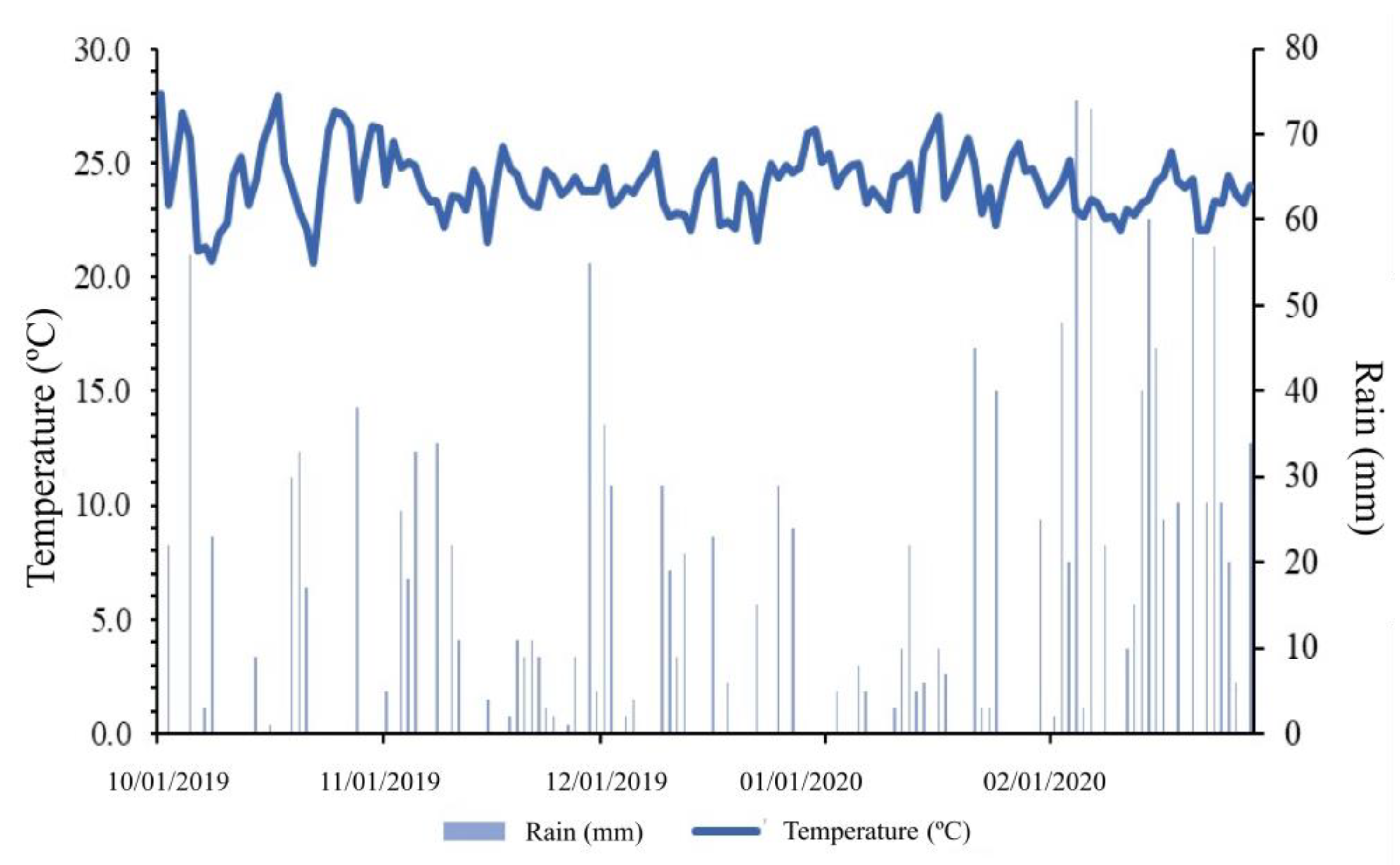
2.1. Conducting the Experiment

The field experiment was carried out in the 2019/20 crop season at the experimental area of the Universidade Federal de Mato Grosso do Sul, municipality of Chapadão do Sul–MS, Brazil, at the coordinates 18°41′33″S and 52°40′45″W, with 810 m of altitude. The region’s soil is classified as Red Dystrophic Latossolo clayey, with the following chemical attributes in the 0–0.20 m layer: pH (H₂O) = 622; exchangeable Al (cmol_c dm⁻³) = 0.0; Ca + Mg (cmol_c dm⁻³) = 4.31; P (mg dm⁻³) = 41.3; K (cmol_c dm⁻³) = 0.2; organic matter (g dm⁻³) = 19.74; V (%) = 45; m (%) = 0.0; sum of bases (cmol_c dm⁻³) = 2.3; and CEC (cmol_c dm⁻³) = 5.1 (Teixeira et al., 2017). According to Koppen’s classification, the region’s climate is Tropical Savanna (Aw). The climatic conditions during the experiment are shown in Figure 1.

A total of 103 F₂ populations of soybean were evaluated in a randomized block design with two repetitions, in which the plants in the central three-meter-long row of each plot were evaluated. The spacing between rows was 0.45 m, and planting density was 15 plants^−m. Sowing was performed in October 2019, adopting the soil preparation system (plowing and harrowing). Seeds were treated with fungicide (Pyraclotrobin + Methyl Thiophanate) and insecticide (Fipronil) at a dose of 200 mL of the commercial product for every 100 kg of seeds to prevent pests and soil fungus. The seeds were also inoculated with bacteria of the Bradyrhizobium genus at a dose of 200 mL of concentrated liquid inoculant for each 100 kg of seeds. Crop treatments were performed according to the needs of the crop.

2.2. Acquisition and Processing of Multispectral Images

When the crop was at 60 days after emergence (DAE), spectral images were collected using a Sensefly eBee RTK fixed-wing remotely piloted aircraft (RPA) with autonomous take-off, flight plan, and landing control. The eBee was equipped with the Parrot Sequoia multispectral sensor. The images were taken at 09:00 am, with cloudless skies, a flight height above ground level of 85 m, and an average field spatial resolution on each picture of 0.089 m, which was adopted for the described survey. The image overlapping was 80% and 65% along- and across-track, respectively. Eighteen ground control points (GCP) markers were placed on the ground surrounding the studying area and surveyed with a pair of the GNSS real-time kinematic (RTK) model Emlid Reach. The RPA average flight speed was 12.5 m/s⁻¹.

Radiometric calibration was performed for the entire scene based on a calibrated reflective target provided by the manufacturer. The Sequoia multispectral sensor also has a light sensor, allowing the calibration of the acquired values for each captured image. The field calibration procedure is performed immediately before the flight is performed. The procedure for taking the reference photo for field calibration is performed by the e-Motion software. The multispectral sensor used was acquired with a horizontal field of view (HFOV) of 61.9°, a vertical field of view (VFOV) of 48.5°, and a diagonal field of view (DFOV) of 73.7°. The reflectance values were obtained in the following spectral bands (SBs): red (640–680 nm), green (530–570 nm), NIR (770–810 nm), and red-edge (730–740 nm). The image resolution is 1280 × 960 pixels, with a pixel size of 3.75 μm and a focal length equal to 3.98 mm. The RMS geolocation errors for X, Y, and Z computed to orthorectify the image were below 0.06 m, with a median of 10,000 keypoints per image. The information acquired by the wavelengths enabled the calculations of the vegetation indices (

Table 1. List of vegetation indices used in the study.

Abbreviation	Vegetation Index	Equation	Ref.
NDVI	Normalized difference vegetation index	$\frac{\left(R_{NIR}–R_{RED}\right)}{\left(R_{NIR}+R_{RED}\right)}$	[22]
NDRE	Normalized difference red-edge index	$\frac{\left(R_{NIR}–R_{EDGE}\right)}{\left(R_{NIR}+R_{EDGE}\right)}$	[23]
GNDVI	Green normalized difference vegetation index	$\frac{\left(R_{NIR}–R_{GREEN}\right)}{\left(R_{NIR}+R_{GREEN}\right)}$	[23]
SAVI	Soil-adjusted vegetation index	$\left(1+0.5\right)\frac{nir-red}{nir+red+0.5}$	[24]
MSAVI	Modified soil-adjusted vegetation index	$\frac{2nir+1-\sqrt{{\left(2nir+1\right)}^2-\left(8nir-red\right)}}{2}$	[25]
MCARI	Modified chlorophyll absorption in reflectance index	$R_{700}-R_{670}-0.2\left(R_{700}-R_{550}\right)\frac{R_{700}}{R_{670}}$	[26]
EVI	Enhanced vegetation index	$2.5\ast \frac{\left(R_{NIR}–R_{RED}\right)}{((R_{NIR})+\left(C1\ast R_{NIR}\right)-\left(\mathrm{C}2\ast R_{BLUE}\right)+\mathrm{L})}$	[27]
SCCCI	Simplified canopy chlorophyll content index	$\frac{\mathrm{NDVI}}{\mathrm{NDRE}}$	[28]

RNIR: near infrared reflectance; RGREEN: green reflectance; RRED: red reflectance; REDGE: red-edge reflectance; L: soil-effect correction factor.

). The images were mosaicked and orthorectified by the computer program Pix4Dmapper.

2.3. Obtaining Nutritional Data

The leaves were washed with water, neutral detergent solution (0.1%), acid solution (HCl 0.3%), and deionized water and then were packed in paper bags and dried in a hot air oven at 65 ± 5 °C until they reached a constant mass. After drying the material, the samples were milled in a Wiley-type mill. Macronutrient analyses (N, P, and K) were performed, following the Bataglia [29] methodology.

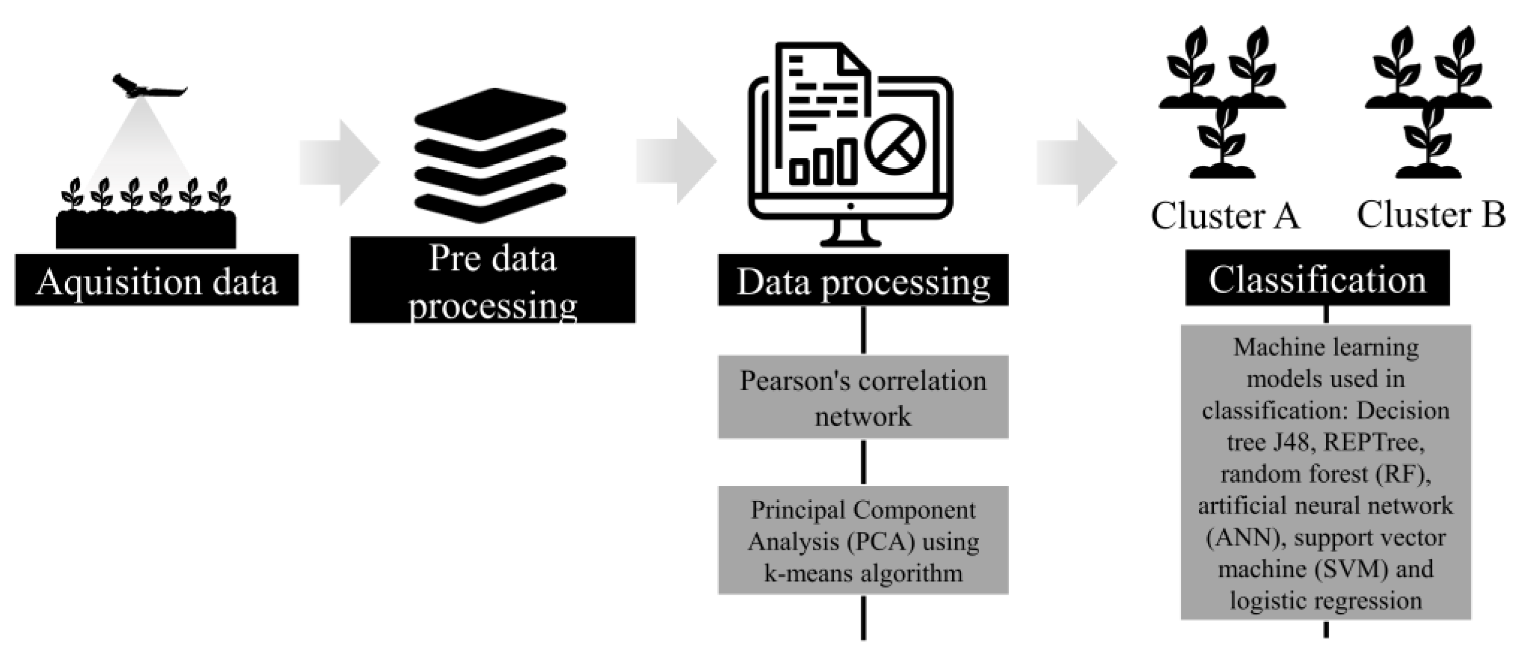
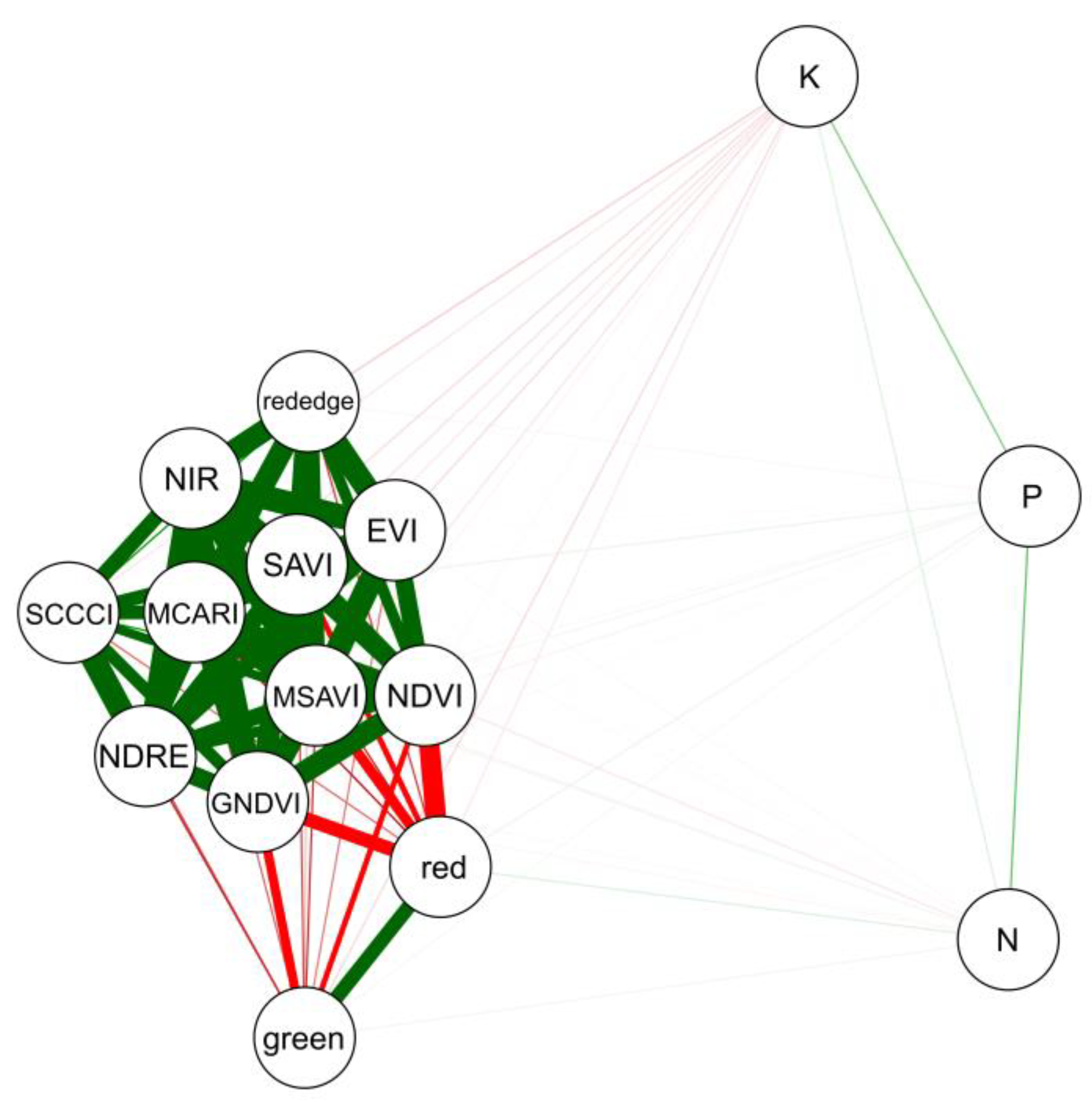
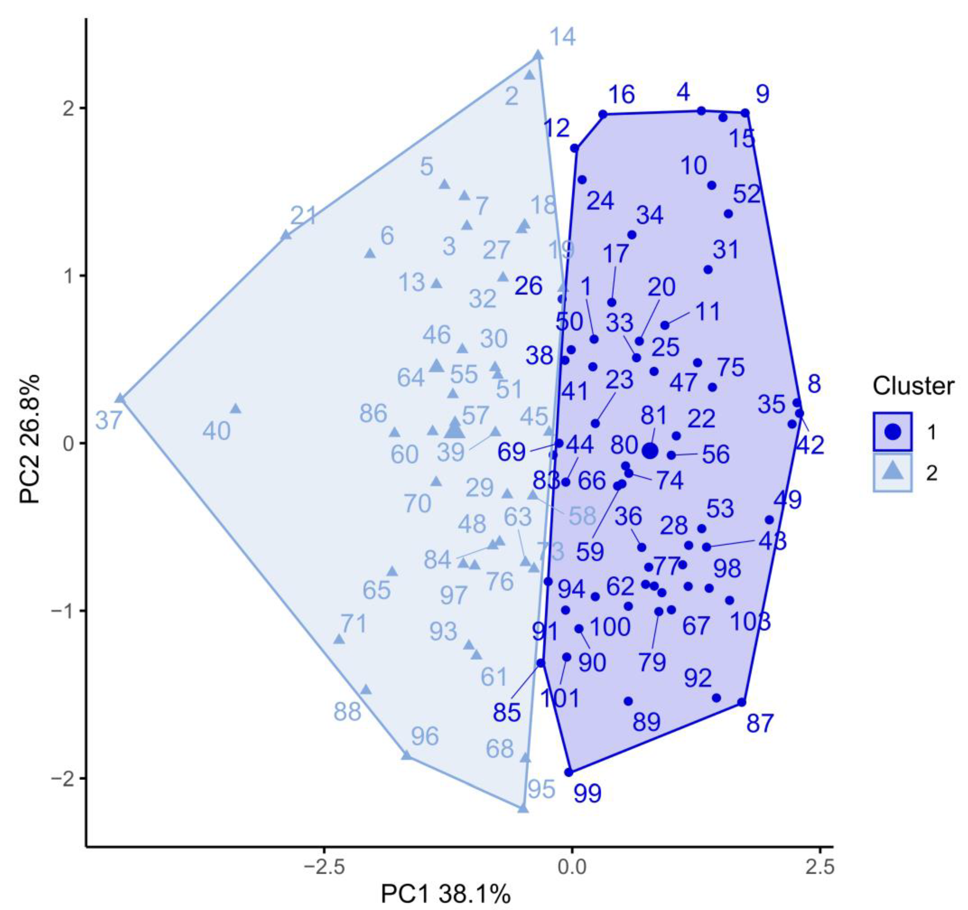
2.4. Statistical Analysis

Once the spectral information and nutritional values of the genotypes for N, P, and K were obtained, data were submitted to a Pearson correlation analysis expressed by a correlation network generated with the Rbio software [30]. For splitting the groups of populations (genotypes), data were submitted to a principal component analysis (PCA) associated with the k-means algorithm. Thus, two clusters were generated: one containing genotypes with higher NPK nutritional values and the other containing genotypes with lower NPK nutritional values. A biplot was generated with the first two components in order to facilitate the interpretation of the results. In this biplot, two clusters (C1 and C2) were defined based on the performance of the genotypes for nutrient contents for further analysis using the k-means algorithm, which clusters treatments whose centroids are closer until there is no significant variation in the minimum distance of each observation to each centroid. These analyses were performed using the “ggfortify” package from the R software [31]. Boxplots were constructed for each cluster according to the content of each nutrient within the groups formed, seeking to observe which set of genotypes had superior nutrient content.

2.5. Machine Learning Models

Afterward, the data were submitted to machine learning analysis (

Table 2. List of machine learning models used in classification.

Abbreviation	Classification Model	Reference
J48	J48 decision tree algorithm	[32]
LR	Logistic regression	[33]
DT	REPTree decision tree algorithm	[34]
RF	Random forest	[35]
ANN	Multilayer perceptron artificial neural network (ANN)	[36]
SVM	Support vector machine	[37]

). A graphic summary of the analyses and the machine learning techniques used is shown in Figure 2. The clusters formed were used as output variables of the classification models used. Spectral data were used as input variables for the models, and three different configurations were tested: using only spectral bands (SB), using only vegetation indices (VI), and using Vis + SBs. Cluster classification was performed using stratified cross-validation with k-fold = 10 and ten repetitions (100 runs for each model). All model parameters were set according to the default setting of the Weka 3.8.5 software.

Model performance was evaluated using the accuracy metrics of percent correct classifications (CC), F-score, and Kappa coefficient. The models’ performances were submitted to an analysis of variance for evaluating the existence of differences between inputs and ML models and the interaction among them. When significant, boxplots were generated with the means grouped by the Scott–Knott test [38] at 5% significance level. The grouping of means and boxplots were generated using the ggplot2 and ExpDes.pt packages of the R software.

3. Results

Pearson’s correlation (Figure 3) shows the positive (green lines) and negative (red lines) relationships between spectral variables and the nutrients evaluated. The thickness of the lines indicates the magnitude of these relationships, with thicker lines representing correlations above 0.6. High-magnitude relationships were among the spectral variables, an expected outcome due to the use of the same spectral bands in the calculations of the vegetation indices. There were positive and low-magnitude correlations among the nutritional variables. There was also a low correlation between spectral variables and nutritional variables.

Soybean genotypes were divided into two groups, cluster 1 and cluster 2, using the k-means algorithm, represented by PCA (Figure 4). Genotypes within the same group have similarities in N, P, and K contents.

The genotypes included in cluster 2 were superior since they presented higher levels for the nutrients studied (Figure 5). The genotypes in cluster 2 can be considered more efficient in the use of nutrients, since with the same fertilization management, these genotypes showed higher values of N (Figure 5a), P (Figure 5b), and K (Figure 5c).

Three accuracy parameters were used to evaluate the performance of the machine learning algorithms: correct classification, F-score, and kappa coefficient. From the analysis of variance (

Table 3. Summary of the analysis of variance for the variables percent correct classification (CC), F-score, and Kappa coefficient.

SV	DF	CC	F-score	Kappa
Inputs	2	0.295	0.0000205	0.00127
ML	5	117.276 *	0.0354062 *	0.013478 *
Inputs *ML	10	5.766	0.0008566 *	0.001641
Residual	162	4.98488	0.0003958	0.00168691

* Significant at 5% probability by F-test; SV: sources of variation; DF: degrees of freedom; ML: machine learning.

), a significant interaction between the inputs and ML algorithms tested for F-score and a significant difference for ML techniques regarding CC and Kappa can be seen.

In the classification of soybean genotypes, the algorithms that had the best performance for correct classification were J48 and SVM (Figure 6a), averaging over 60% accuracy. RF had the worst performance among the algorithms, averaging around 55% accuracy. J48, DT, RF, and SVM algorithms had the best Kappa performances (Figure 6b).

The tested inputs showed no significant difference for the J48, DT, ANN, and SVM algorithms (Figure 7). Regarding the LR algorithm, the input containing only spectral bands showed better performance. The input containing both spectral bands and vegetation indices performed best using the RF algorithm. By evaluating the MLs within each input, the J48 decision tree and SVM algorithms performed well regardless of the input used. RF was the algorithm that achieved the worst performance regardless of the input tested.

The use of SB showed no difference compared with that of the other inputs tested (Figure 7). Therefore, a confusion matrix was developed (Figure 8) for each algorithm, using SB as input for the models. Values with dark blue shades show the number of correct classifications obtained for each cluster, while lighter blue shades show the error rate for the best configuration of each algorithm.

It is possible to observe that the algorithms J48, LR, DT, RF, and ANN were similar regarding the correct classifications of the genotypes in clusters C1 and C2, being superior to SVM. However, it is important to highlight that ANN had a lower error rate (12 incorrect classifications) than the other algorithms.

4. Discussion

The spectral and nutritional data showed a low correlation with each other due to the complex interaction between the data (Figure 3). Unlike traditional statistical methods, such as the Pearson correlation, machine learning (ML) algorithms perform well when processing non-linear and non-parametric data, such as plant nutritional analysis and spectral data [39]. Given this, the genotypes were separated into two clusters (Figure 4).

Fertilization management for all genotypes was the same. However, after separating the genotypes into clusters, it was observed that the genotypes belonging to cluster 2 had a higher content of the nutrients evaluated. The current soybean cultivars differ in several characteristics, including the ability to uptake and metabolize nutrients [40]. Using remote sensing technologies coupled with computational advances in data analysis is a crucial way to implement fertilization management in agriculture, allowing the spatiotemporal evaluation of several plant characteristics in an economical and fast way [41].

The availability of N, P, and K in Brazilian soils is limited. Thus, monitoring these elements in a fast, accurate, and non-destructive way allows information to be obtained at different phenological stages of the crop, providing efficient fertilization management [42]. The evaluation and mapping of these nutrients are essential for monitoring crop production in the field, making it crucial to develop methods for monitoring, evaluating, and measuring these nutrient contents in a fast, accurate, low-cost, and non-destructive way [41]. Promoting the development of crops that are more efficient in using these resources [43] is a path to be followed in soybean breeding programs seeking genotypes efficient in nutrient uptake, enabling more sustainable agriculture without affecting the grain yield [44].

Classifying the genotypes according to nutritional contents may contribute significantly to breeding programs, facilitating the selection of genotypes. However, this evaluation requires many leaf samples, which can be reduced if this information is obtained through spectral data [11]. The use of ML techniques in processing this information is essential to deal efficiently with the number of genotypes evaluated and the number of spectral data generated. ML techniques can also deal accurately with the lack of linearity between nutritional and spectral data [39]. Using ML techniques associated with spectral data makes it possible to obtain important information from the leaves associated with the health and nutritional content of the plants [39]. Thus, it is possible to have a reliable diagnosis of the nutritional state of soybean, allowing greater accuracy in the fertilization management on farms, contributing to the improve the crop yield [19].

In our study, the J48 and SVM algorithms performed best in all accuracy metrics evaluated (Figure 6a,b and Figure 7). The J48 algorithm provides classification results efficiently and quickly from a processing point of view [45]. In addition to the lower time demand for data processing, there is a lower need for human interference in constructing the algorithm [46]. SVM has shown good performance and robustness in classification using spectral data [47,48] and good generalization ability and accuracy [49].

All three inputs tested provided better performance for the J48 and SVM algorithms. Since there was no difference between the inputs tested, it is more practical to use SB from a processing point of view. According to [20], using spectral bands as input for ML models is more feasible because there is no need to perform vegetation index calculations. Spectral bands are efficiently used to determine several plant characteristics, such as the water status in soybean plants [50] and the nutritional status with regards to boron deficiency, appropriate range, and toxicity in eucalyptus plants [21]. Thus, the use of spectral data makes it possible to detect changes in the leaf at nutritional level, and with the support of appropriate technologies, other important information can be provided. ML techniques, when properly used, have been shown to overcome several classification problems [19].

Thus, the spectral bands provide essential information about the nutritional state of soybean plants. Through this data, combined with the use of ML techniques, it is possible to classify soybean genotypes according to their nitrogen, phosphorus, and potassium status. In this way, it is possible to assist improvement programs in a cost-effective manner to develop soybean cultivars that are efficient in uptaking and metabolizing these nutrients, reducing the use of mineral fertilizers. Thus, this practice can generate savings for farmers and mitigate environmental impacts caused by excess contamination from using such fertilizers.

ML techniques and multispectral data can accurately provide several pieces of information about the crops, giving guidelines for crop management still in the field [51]. For future works, it is necessary that further genotypes be assessed, observing the behavior of ML algorithms with information from different crops, fertilization managements, and nutrients. Although the results reported here are promising for classifying soybean genotypes for primary macronutrients, we suggest that future research use hyperspectral sensors for such evaluations, as these provide higher quantities of SB, which may improve prediction accuracy.

5. Conclusions

The classification of soybean genotypes according to the nutritional contents of primary macronutrients (N, P, and K) from spectral data is a complex task due to the lack of linear relationship between such variables, which is easily overcome by ML algorithms. The input information of these algorithms is also important for their better accuracy. Algorithms J48 and SVM showed the best performance in classifying soybean genotypes. In addition to the algorithms, three different inputs (spectral bands, vegetation index, and spectral bands + vegetation indices) were tested to verify which spectral data provide the best classification accuracy. The best input configuration for the ML algorithms was to use spectral bands as input for the algorithms, achieving better performance in identifying groups of genotypes in terms of their nutritional content. Thus, the use of spectral bands in the J48 and SVM algorithms allows a fast, accurate, and non-destructive classification of soybean genotypes for N, P, and K contents.

References

1. Lynch, J.P. Root Phenes That Reduce the Metabolic Costs of Soil Exploration: Opportunities for 21st Century Agriculture. Plant Cell Environ. 2015, 38, 1775–1784. [Google Scholar] [CrossRef] [PubMed]
2. Zhou, S.; Mou, H.; Zhou, J.; Zhou, J.; Ye, H.; Nguyen, H.T. Development of an Automated Plant Phenotyping System for Evaluation of Salt Tolerance in Soybean. Comput. Electron. Agric. 2021, 182, 106001. [Google Scholar] [CrossRef]
3. Der Yang, M.; Tseng, H.H.; Hsu, Y.C.; Yang, C.Y.; Lai, M.H.; Wu, D.H. A UAV Open Dataset of Rice Paddies for Deep Learning Practice. Remote Sens. 2021, 13, 1358. [Google Scholar] [CrossRef]
4. Panday, U.S.; Pratihast, A.K.; Aryal, J.; Kayastha, R.B. A Review on Drone-Based Data Solutions for Cereal Crops. Drones 2020, 4, 41. [Google Scholar] [CrossRef]
5. Guo, Y.; Chen, S.; Li, X.; Cunha, M.; Jayavelu, S.; Cammarano, D.; Fu, Y. Machine Learning-Based Approaches for Predicting SPAD Values of Maize Using Multi-Spectral Images. Remote Sens 2022, 14, 1337. [Google Scholar] [CrossRef]
6. Everaerts, J. The Use of Unmanned Aerial Vehicles (UAVs) for Remote Sensing and Mapping. Int. Arch. Photogramm. Remote Sens. Spat. Inf. Sci. 2008, 37, 1187–1192. [Google Scholar]
7. Ling, B.; Goodin, D.G.; Raynor, E.J.; Joern, A. Hyperspectral Analysis of Leaf Pigments and Nutritional Elements in Tallgrass Prairie Vegetation. Front Plant. Sci. 2019, 10, 142. [Google Scholar] [CrossRef] [Green Version]
8. Moreno, R.; Corona, F.; Lendasse, A.; Graña, M.; Galvão, L.S. Extreme Learning Machines for Soybean Classification in Remote Sensing Hyperspectral Images. Neurocomputing 2014, 128, 207–216. [Google Scholar] [CrossRef]
9. Mahajan, G.R.; Das, B.; Murgaokar, D.; Herrmann, I.; Berger, K.; Sahoo, R.N.; Patel, K.; Desai, A.; Morajkar, S.; Kulkarni, R.M. Monitoring the Foliar Nutrients Status of Mango Using Spectroscopy-Based Spectral Indices and PLSR-Combined Machine Learning Models. Remote Sens. 2021, 13, 641. [Google Scholar] [CrossRef]
10. O’Connell, J.L.; Byrd, K.B.; Kelly, M. Remotely-Sensed Indicators of N-Related Biomass Allocation in Schoenoplectus Acutus. PLoS ONE 2014, 9, e90870. [Google Scholar] [CrossRef]
11. Osco, L.P.; Marques Ramos, A.P.; Saito Moriya, É.A.; de Souza, M.; Marcato Junior, J.; Matsubara, E.T.; Imai, N.N.; Creste, J.E. Improvement of Leaf Nitrogen Content Inference in Valencia-Orange Trees Applying Spectral Analysis Algorithms in UAV Mounted-Sensor Images. Int. J. Appl. Earth Obs. Geoinf. 2019, 83, 101907. [Google Scholar] [CrossRef]
12. Hawkesford, M.; Horst, W.; Kichey, T.; Lambers, H.; Schjoerring, J.; Møller, I.S.; White, P. Chapter 6—Functions of Macronutrients. In Marschner’s Mineral Nutrition of Higher Plants (Third Edition); Marschner, P., Ed.; Academic Press: San Diego, CA, USA, 2012; pp. 135–189. ISBN 978-0-12-384905-2. [Google Scholar]
13. Mukherjee, S.; Laskar, S. Vis–NIR-Based Optical Sensor System for Estimation of Primary Nutrients in Soil. J. Opt. 2019, 48, 87–103. [Google Scholar] [CrossRef]
14. Amirruddin, A.D.; Muharam, F.M.; Ismail, M.H.; Tan, N.P.; Ismail, M.F. Hyperspectral Spectroscopy and Imbalance Data Approaches for Classification of Oil Palm’s Macronutrients Observed from Frond 9 and 17. Comput. Electron. Agric. 2020, 178, 105768. [Google Scholar] [CrossRef]
15. Pham, B.T.; Tien Bui, D.; Prakash, I.; Dholakia, M.B. Hybrid Integration of Multilayer Perceptron Neural Networks and Machine Learning Ensembles for Landslide Susceptibility Assessment at Himalayan Area (India) Using GIS. Catena 2017, 149, 52–63. [Google Scholar] [CrossRef]
16. Camps-Valls, G. Machine Learning in Remote Sensing Data Processing. In Proceedings of the 2009 IEEE International Workshop on Machine Learning for Signal Processing, Grenoble, France, 1–4 September 2009; pp. 1–6. [Google Scholar]
17. de Medeiros, A.D.; Capobiango, N.P.; da Silva, J.M.; da Silva, L.J.; da Silva, C.B.; dos Santos Dias, D.C.F. Interactive Machine Learning for Soybean Seed and Seedling Quality Classification. Sci. Rep. 2020, 10, 11267. [Google Scholar] [CrossRef] [PubMed]
18. Orusa, T.; Cammareri, D.; Borgogno Mondino, E. A Scalable Earth Observation Service to Map Land Cover in Geomorphological Complex Areas beyond the Dynamic World: An Application in Aosta Valley (NW Italy). Appl. Sci. 2023, 13, 390. [Google Scholar] [CrossRef]
19. Barbedo, J.G.A. Detection of Nutrition Deficiencies in Plants Using Proximal Images and Machine Learning: A Review. Comput. Electron. Agric. 2019, 162, 482–492. [Google Scholar] [CrossRef]
20. Gava, R.; Santana, D.C.; Cotrim, M.F.; Rossi, F.S.; Teodoro, L.P.R.; da Silva Junior, C.A.; Teodoro, P.E. Soybean Cultivars Identification Using Remotely Sensed Image and Machine Learning Models. Sustainability 2022, 14, 7125. [Google Scholar] [CrossRef]
21. Da Silva Junior, C.A.; Teodoro, P.E.; Teodoro, L.P.R.; Della-Silva, J.L.; Shiratsuchi, L.S.; Baio, F.H.R.; Boechat, C.L.; Capristo-Silva, G.F. Is It Possible to Detect Boron Deficiency in Eucalyptus Using Hyper and Multispectral Sensors? Infrared Phys. Technol. 2021, 116, 103810. [Google Scholar] [CrossRef]
22. Rouse, J.W.; Haas, R.H.; Schell, J.A.; Deering, D.W. Monitoring Vegetation Systems in the Great Plains with ERTS. NASA Spec. Publ. 1974, 351, 309. [Google Scholar]
23. Gitelson, A.A.; Kaufman, Y.J.; Merzlyak, M.N. Use of a Green Channel in Remote Sensing of Global Vegetation from EOS-MODIS. Remote Sens. Environ. 1996, 58, 289–298. [Google Scholar] [CrossRef]
24. Huete, A.R. A Soil-Adjusted Vegetation Index (SAVI). Remote Sens. Environ. 1988, 25, 295–309. [Google Scholar] [CrossRef]
25. Qi, J.; Chehbouni, A.; Huete, A.R.; Kerr, Y.H.; Sorooshian, S. A Modified Soil Adjusted Vegetation Index. Remote Sens. Environ. 1994, 48, 119–126. [Google Scholar] [CrossRef]
26. Daughtry, C.S.T.; Walthall, C.L.; Kim, M.S.; de Colstoun, E.B.; McMurtrey Iii, J.E. Estimating Corn Leaf Chlorophyll Concentration from Leaf and Canopy Reflectance. Remote Sens. Environ. 2000, 74, 229–239. [Google Scholar] [CrossRef]
27. Huete, A.R.; Liu, H.Q.; Batchily, K.V.; van Leeuwen, W. A Comparison of Vegetation Indices over a Global Set of TM Images for EOS-MODIS. Remote Sens. Environ. 1997, 59, 440–451. [Google Scholar] [CrossRef]
28. Raper, T.B.; Varco, J.J. Canopy-Scale Wavelength and Vegetative Index Sensitivities to Cotton Growth Parameters and Nitrogen Status. Precis. Agric. 2015, 16, 62–76. [Google Scholar] [CrossRef] [Green Version]
29. Bataglia, O.C.; Teixeira, J.P.F.; Furlani, P.R.; Furlani, A.M.C.; Gallo, J.R. Métodos de Análise Química de Plantas; IAC: Campinas, Brasil, 1978; Volume 87. [Google Scholar]
30. Bhering, L.L. Rbio: A Tool for Biometric and Statistical Analysis Using the R Platform. Crop. Breed. Appl. Biotechnol. 2017, 17, 187–190. [Google Scholar] [CrossRef] [Green Version]
31. Team, R.C. R: A Language and Environment for Statistical Computing. Comput. Sci. Rev. 2013, 201, 1–12. [Google Scholar]
32. Quinlan, J.R. C4. 5: Programming for Machine Learning. Morgan Kauffmann 1993, 38, 49. [Google Scholar]
33. Štepanovský, M.; Ibrová, A.; Buk, Z.; Velemínská, J. Novel Age Estimation Model Based on Development of Permanent Teeth Compared with Classical Approach and Other Modern Data Mining Methods. Forensic. Sci. Int. 2017, 279, 72–82. [Google Scholar] [CrossRef]
34. Al Snousy, M.B.; El-Deeb, H.M.; Badran, K.; Al Khlil, I.A. Suite of Decision Tree-Based Classification Algorithms on Cancer Gene Expression Data. Egypt. Inform. J. 2011, 12, 73–82. [Google Scholar] [CrossRef] [Green Version]
35. Belgiu, M.; Drăguţ, L. Random Forest in Remote Sensing: A Review of Applications and Future Directions. ISPRS J. Photogramm. Remote Sens. 2016, 114, 24–31. [Google Scholar] [CrossRef]
36. Egmont-Petersen, M.; de Ridder, D.; Handels, H. Image Processing with Neural Networks—A Review. Pattern. Recognit. 2002, 35, 2279–2301. [Google Scholar] [CrossRef]
37. Nalepa, J.; Kawulok, M. Selecting Training Sets for Support Vector Machines: A Review. Artif. Intell. Rev. 2019, 52, 857–900. [Google Scholar] [CrossRef] [Green Version]
38. Scott, A.J.; Knott, M. A Cluster Analysis Method for Grouping Means in the Analysis of Variance. Biometrics 1974, 30, 507–512. [Google Scholar] [CrossRef] [Green Version]
39. Osco, L.P.; Ramos, A.P.M.; Faita Pinheiro, M.M.; Moriya, É.A.S.; Imai, N.N.; Estrabis, N.; Ianczyk, F.; de Araújo, F.F.; Liesenberg, V.; Jorge, L.A.d.A. A Machine Learning Framework to Predict Nutrient Content in Valencia-Orange Leaf Hyperspectral Measurements. Remote Sens. 2020, 12, 906. [Google Scholar] [CrossRef] [Green Version]
40. Chaney, R.L. Breeding Soybeans to Prevent Mineral Deficiencies or Toxicities. In World Soybean Research Conference III: Proceedings, Ames, IA, 12–17 August 1984; CRC Press: Boca Raton, FL, USA, 2022; pp. 453–459. [Google Scholar]
41. Khechba, K.; Laamrani, A.; Dhiba, D.; Misbah, K.; Chehbouni, A. Monitoring and Analyzing Yield Gap in Africa through Soil Attribute Best Management Using Remote Sensing Approaches: A Review. Remote Sens. 2021, 13. [Google Scholar] [CrossRef]
42. Peng, X.; Chen, D.; Zhou, Z.; Zhang, Z.; Xu, C.; Zha, Q.; Wang, F.; Hu, X. Prediction of the Nitrogen, Phosphorus and Potassium Contents in Grape Leaves at Different Growth Stages Based on UAV Multispectral Remote Sensing. Remote Sens. 2022, 14, 2659. [Google Scholar] [CrossRef]
43. Soba, D.; Shu, T.; Runion, G.B.; Prior, S.A.; Fritschi, F.B.; Aranjuelo, I.; Sanz-Saez, A. Effects of Elevated [CO2] on Photosynthesis and Seed Yield Parameters in Two Soybean Genotypes with Contrasting Water Use Efficiency. Environ. Exp. Bot 2020, 178, 104154. [Google Scholar] [CrossRef]
44. Xiong, R.; Liu, S.; Considine, M.J.; Siddique, K.H.M.; Lam, H.-M.; Chen, Y. Root System Architecture, Physiological and Transcriptional Traits of Soybean (Glycine Max L.) in Response to Water Deficit: A Review. Physiol. Plant 2021, 172, 405–418. [Google Scholar] [CrossRef]
45. Rossi Neto, J.; de Souza, Z.M.; de Medeiros Oliveira, S.R.; Kölln, O.T.; Ferreira, D.A.; Carvalho, J.L.N.; Braunbeck, O.A.; Franco, H.C.J. Use of the Decision Tree Technique to Estimate Sugarcane Productivity Under Edaphoclimatic Conditions. Sugar Tech. 2017, 19, 662–668. [Google Scholar] [CrossRef]
46. Vieira, M.A.; Formaggio, A.R.; Rennó, C.D.; Atzberger, C.; Aguiar, D.A.; Mello, M.P. Object Based Image Analysis and Data Mining Applied to a Remotely Sensed Landsat Time-Series to Map Sugarcane over Large Areas. Remote Sens. Environ. 2012, 123, 553–562. [Google Scholar] [CrossRef]
47. Bigdeli, B.; Samadzadegan, F.; Reinartz, P. A Multiple SVM System for Classification of Hyperspectral Remote Sensing Data. J. Indian Soc. Remote Sens. 2013, 41, 763–776. [Google Scholar] [CrossRef] [Green Version]
48. Okwuashi, O.; Ndehedehe, C.E. Deep Support Vector Machine for Hyperspectral Image Classification. Pattern. Recognit. 2020, 103, 107298. [Google Scholar] [CrossRef]
49. Mountrakis, G.; Im, J.; Ogole, C. Support Vector Machines in Remote Sensing: A Review. ISPRS J. Photogramm. Remote Sens. 2011, 66, 247–259. [Google Scholar] [CrossRef]
50. Braga, P.; Crusiol, L.G.T.; Nanni, M.R.; Caranhato, A.L.H.; Fuhrmann, M.B.; Nepomuceno, A.L.; Neumaier, N.; Farias, J.R.B.; Koltun, A.; Gonçalves, L.S.A.; et al. Vegetation Indices and NIR-SWIR Spectral Bands as a Phenotyping Tool for Water Status Determination in Soybean. Precis. Agric. 2021, 22, 249–266. [Google Scholar] [CrossRef]
51. Bian, C.; Shi, H.; Wu, S.; Zhang, K.; Wei, M.; Zhao, Y.; Sun, Y.; Zhuang, H.; Zhang, X.; Chen, S. Prediction of Field-Scale Wheat Yield Using Machine Learning Method and Multi-Spectral UAV Data. Remote Sens. 2022, 14, 1474. [Google Scholar] [CrossRef]
Figure 1. Weather conditions over the 2019/2020 crop season.
Remotesensing 15 01457 g001
Figure 2. Summary of processes carried out in data analysis.
Remotesensing 15 01457 g002
Figure 3. Pearson’s correlation network between the nutritional (potassium–K, phosphorus–P, and nitrogen–N content) and spectral variables (spectral bands and vegetation index). Variables connected by green lines are positively correlated, while variables connected by red lines are negatively correlated. The thickness of the line is proportional to the magnitude of the correlation.
Remotesensing 15 01457 g003
Figure 4. Principal component (PC) analysis for the clusters formed, according to the potassium, phosphorus, and nitrogen content of the soybean genotypes (numbers of 1 to 103) using the k-means algorithm.
Remotesensing 15 01457 g004
Figure 5. Boxplot with the means of nitrogen–N (a), phosphorus–P (b), and potassium–K (c) content for the clusters formed.
Remotesensing 15 01457 g005
Figure 6. Boxplot of the clustering of means for percent correct classification–CC (a) and Kappa coefficient (b), regarding the machine learning models tested (J48 decision tree algorithm–J48, logistic regression–LR, REPTree decision tree algorithm–DT, random forest–RF, multilayer perceptron artificial neural network–ANN, and support vector machine–SVM). Means followed by the same letters do not differ by the Scott–Knott test at 5% probability.
Remotesensing 15 01457 g006
Figure 7. Boxplot of the clustering of means for F-score regarding the machine learning models tested (J48 decision tree algorithm–J48, logistic regression–LR, REPTree decision tree algorithm–DT, random forest–RF, multilayer perceptron artificial neural network–ANN, and support vector machine–SVM). Means followed by the same letters do not differ by the Scott–Knott test at 5% probability.
Remotesensing 15 01457 g007
Figure 8. Confusion matrix to classify the clusters formed for the soybean genotypes for machine learning models tested (J48 decision tree algorithm–J48 (a), logistic regression–LR (b), REPTree decision tree algorithm–DT (c), random forest–RF (d), multilayer perceptron artificial neural network–ANN (e), and support vector machine–SVM (f)) using the spectral bands as inputs. The main diagonal shows the number of correct classifications in each cluster.
Remotesensing 15 01457 g008