Article

An Adaptive Adversarial Patch-Generating Algorithm for Defending against the Intelligent Low, Slow, and Small Target

1
Unmanned System Research Institute, Northwestern Polytechnical University, Xi’an 710072, China
2
School of Electronics And Information, Northwestern Polytechnical University, Xi’an 710072, China
*
Author to whom correspondence should be addressed.
Remote Sens. 2023, 15(5), 1439; https://doi.org/10.3390/rs15051439
Submission received: 11 January 2023 / Revised: 21 February 2023 / Accepted: 23 February 2023 / Published: 3 March 2023
(This article belongs to the Special Issue Adversarial Attacks and Defenses for Remote Sensing Data)

Abstract

:
The “low, slow, and small” target (LSST) poses a significant threat to the military ground unit. It is hard to defend against due to its invisibility to numerous detecting devices. With the onboard deep learning-based object detection methods, the intelligent LSST (ILSST) can find and detect the ground unit autonomously in a denied environment. This paper proposes an adversarial patch-based defending method to blind the ILSST by attacking its onboard object detection network. First, an adversarial influence score was established to indicate the influence of the adversarial noise on the objects. Then, based on this score, we used the least squares algorithm and Bisectional search methods to search the patch’s optimal coordinates and size. Using the optimal coordinates and size, an adaptive patch-generating network was constructed to automatically generate patches on ground units and hide the ground units from the deep learning-based object detection network. To evaluate the efficiency of our algorithm, a new LSST view dataset was collected, and extensive attacking experiments are carried out on this dataset. The results demonstrate that our algorithm can effectively attack the object detection networks, is better than state-of-the-art adversarial patch-generating algorithms in hiding the ground units from the object detection networks, and has high transferability among the object detection networks.

1. Introduction

The “low, slow, and small” target (LSST) is the abbreviation of the low-altitude, slow-speed, and small target. It refers to the aerial target with a flying height of less than 1000 m, a flight speed of less than 200 km/h, and a radar reflection cross-sectional of less than 2 m2 [1]. They can be divided into multi-rotor, fixed-wing, and small unmanned helicopters. Along with the geometric growth of the drone market, the frequency of the incidents such as “black flight,” border cross, and drone attacks is increasing [2]. Moreover, if these drones are equipped with an intelligent system, they can operate independently in the denied environments [3,4].
Currently, the countermeasures against LSST are mainly based on kinetic and non-kinetic countermeasures.
The kinetic countermeasures mainly utilize small arms to destroy, interceptors to intercept, or aerial nets to capture LSST. All of these countermeasures depend on LSST detection. The detection of LSST is mainly based on radar [5,6], audio [7,8], video [9,10], and radio frequency [11,12].
Radar: The micro-doppler signal received using the doppler radar can help to identify the LSST [13]. However, because the LSST has a low radar cross-section, the detection of LSST using the radar faces significant challenges.
Audio: Analyzing the sound waves generated by LSST’s rotor can detect the LSST [14]. Although this can realize 24/7 uninterrupted detection, its detection range is not satisfiable and vulnerable to background noise.
Video: Computer vision technology enabled LSST detection [15,16] based on video images and object detection algorithms. However, it has a limited detection range and is vulnerable to rainy, foggy, and dusty weather.
Radio frequency: The LSST usually uses some special frequency band to communicate with their controllers [17]. By using a radio frequency scanning technic, one can monitor the LSST. However, in a real-world environment, a lot of radio frequency signals will lead to a high false alarm rate, making this technology unreliable on LSST detection tasks.
The non-kinetic countermeasures mainly use some interrupting technology to disturb the LSST. It mainly disrupts the control links to make the LSST out of control [18] or sends a false GPS signal [19] to make the LSST deviate from its route. However, intelligent LSST (ILSST) navigation mainly depends on a visual navigation system that does not rely on a GPS signal to navigate itself. It can operate on its own and barely require remote controls. Therefore, these LSSTs equipped with intelligent systems are nearly free from these kinds of disturbances.
ILSSTs are usually equipped with an object detection algorithm to locate ground units. To defend against the ILSST, we propose an adaptive adversarial patch-generating algorithm to make the ground unit invisible to the ILSST’s object detection algorithm. Due to its low speed, the ILSST can endure the latency of the object detection network. In exchange, it will achieve high detection precision. However, to guarantee real-time operation ability, the complexity of the network cannot be too high. Currently, few object detection networks can meet the requirement. Among them, due to its high precision, low complexity, and whole package of the solution to deploy on an embedded system, the YOLOv5 [20] algorithm is an optimal solution to use on the ILSST.
Therefore, this paper proposes an algorithm to attack the YOLOv5 network, which can hide the ground units from YOLOv5 and has high transferability among the other object detection networks. To our knowledge, this is the first time the adversarial patch has been used to defend against ILSST, which can protect critical ground units or facilities from being discovered or attacked by ILSST.
The overall structure of our proposed algorithm is shown in Figure 1. Our proposed algorithm in this paper consists of two parts: (1) the dataset labeling part provides the optimal coordinate and the size of the adversarial patches to the training dataset, as shown in the upper part of Figure 1; (2) the adaptive adversarial patch-generating network uses the labeled training dataset to construct a patch-generating model as shown in the lower part of Figure 1. Our contributions are as follows:
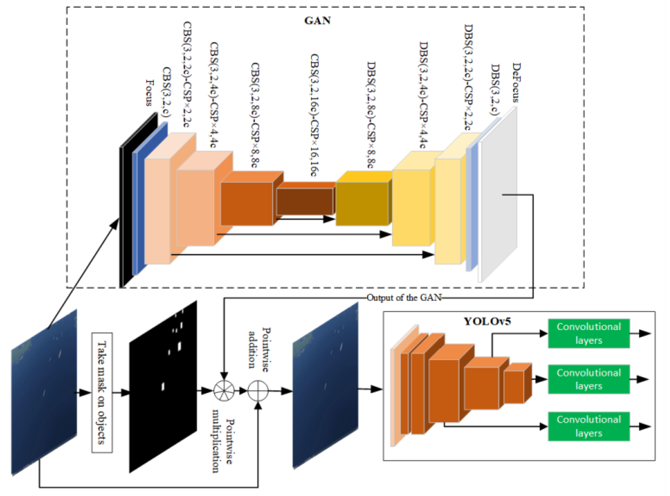
  • We propose a novel idea for defending against the ILSST. Using the adversarial patch to defend against the ILSST can hide the ground unit from ILSST’s onboard object detection network.
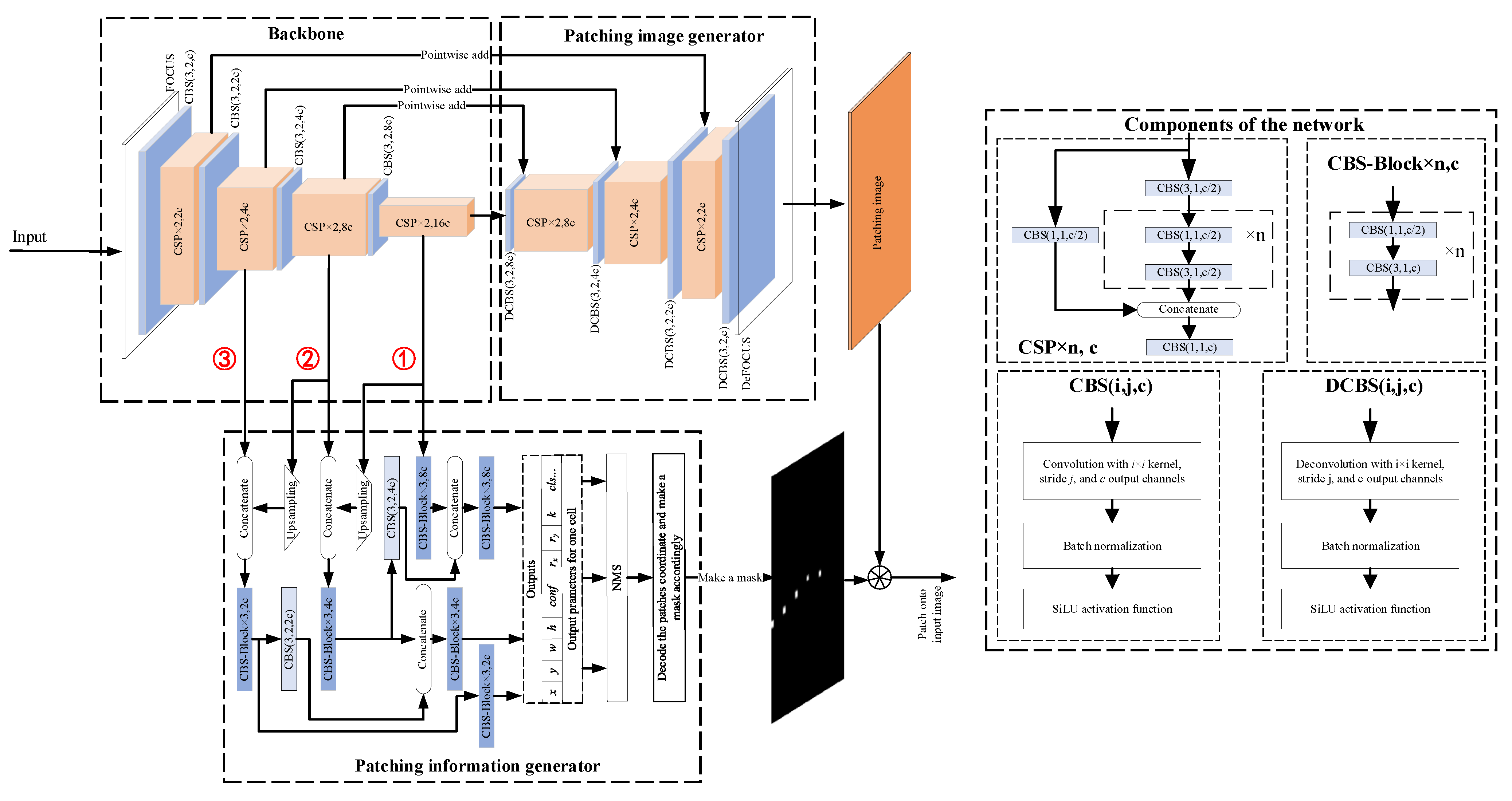
  • We design a patch-generating network that can generate patches on the optimal location of the object with optimal size without the ground truth of the objects.
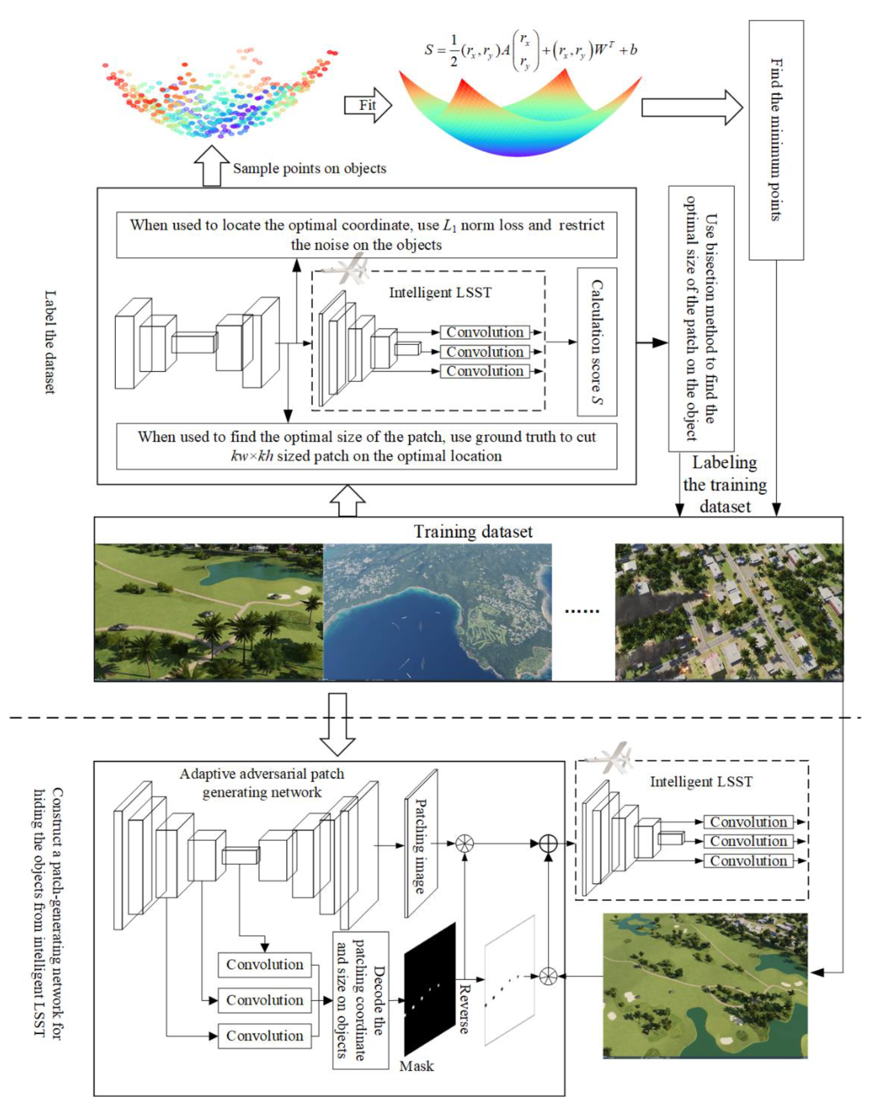
  • We propose a novel patch coordinate labeling method that fits a curve to an object using a set of sampling points and use this curve to find the point that affects the detection results most.
  • We use the Bisectional search method to calculate the optimal size of the patch on objects, which enable our algorithm to generate different sized patch on different objects and increase the efficiency of the patch-generating algorithm.
Our paper is arranged as follows. In Section 2, we describe some of the related work on adversarial attacks and provide a detailed description of our algorithm. In Section 3, we experimentally evaluate our algorithm. Finally, we give the discussion and conclusion in Section 4.

2. Materials and Methods

2.1. Related Work

Recently, adversarial attacks have become an important concern in the field of computer vision and pose a significant threat to the remote sensing field as well. Consequently, adversarial attacks in remote sensing have become a growing concern in recent years [21]. Researchers have proposed various methods to generate adversarial examples that can deceive deep neural networks in remote sensing applications. Firstly, we summarize the adversarial attack algorithms, including adversarial perturbations and adversarial patches in classification and object detection tasks. Secondly, we review the application of adversarial attacks in remote sensing.
Adversarial perturbation: This type of attack misleads the network to give a wrong prediction by adding the imperceptible micro-noise to a normal sample. For the classification, there is much research. Szegedy [22] first discovered the adversarial phenomenon on image classification tasks and proposed an adversarial sample generating method L-BFGS. Based on this research, the fast gradient sign method (FGSM) has been proposed by Goodfellow [23]. FGSM adds perturbation along with the direction of the gradient. Its simplicity and efficiency have stimulated several pieces of research based on it [24,25]. These methods did not have much difference from the original FGSM algorithm. DeepFool algorithm [26] generates noise by comparing the distance between the points in sample spaces and the classification boundaries. The Jacobian-based saliency map attacks (JSMA) algorithm [27] calculates the salient scores on inputting images and adds perturbations according to the importance of the pixel to the output result, which can deceive the classification algorithm by merely changing a few pixels. C&W algorithm [28] uses the improved norms as the loss function to optimize the perturbation. Afterward, Rony et al. [29] improve the C&W algorithm to increase adversarial ability while still obtaining samples that approximate the visual perceptibility of the original algorithm. Croce et al. [30] proposed two algorithms, the auto-projected gradient descent, and the AutoAttacks, based on analysis of the suboptimal solutions phenomenon. Xiao et al. [31] proposes a generative adversarial network (GAN)-based method to efficiently generate stronger and more diverse examples for deep neural networks. Bai et al. [32] leverage both gradient-based and gradient-free optimization techniques to generate adversarial examples that are effective and transferable across multiple deep-learning models. Liu et al. [32] highly considers human perception and improves the inconspicuousness and transferability of generated patches. These described algorithms are typical classification attack algorithms; in this work, we concentrate on attacking the object detection algorithms.
For object detection algorithms, the research are not as much for attacking classification algorithms. Xie et al. [33] proposed an adversarial sample generation method for object detection algorithms. They proposed a dense adversarial generation algorithm that considers all objects simultaneously and optimizes the overall loss function to increase the transferability between object detection models. To attack a region proposal-based object detection algorithm, Li et al. [34] proposed the Robust Adversarial Perturbation (RAP). They construct two loss functions, one for the label and the other one for the shape. They implement an attack on region proposal-based object detection algorithms by optimizing these two loss functions. In order to speed up the attacking method and deal with the problem that the method used to attack region proposal-based object detection algorithm cannot attack regression-based object detection algorithm, Wei et al. [35] proposed the Unified and Efficient Adversary (UEA). The UEA is based on Generative Adversarial Network (GAN) [36] and combines high-level classification and low-level feature loss to jointly train an adversarial sample generator. Athalye et al. [37] generated three-dimensional adversarial samples to mislead the neural network by using the concept of “Expectation over Transformation” (EoT). Wang et al. [38] proposed a method that can attack the object detection algorithm that uses the Non-Maximum Suppression (NMS) method to filter out the redundant bounding box. Compressing the dimension of detection boxes, they paralyzed the NMS to make the detection result full of false positives. Although these object detection algorithms attacking methods can attack the object detection methods, they cannot be implemented in real-world circumstances because the perturbations added to the original image are too subtle to be captured by a camera.
Adversarial patch: This type of attack uses some specific-colored patches to replace an area in an image, which can mislead the network to give a false prediction. Currently, several breakthroughs have been made in the research of adversarial patches. Firstly, we summarize the adversarial patch-based attack for classification tasks. Brown et al. [39] propose adding a small patch to an image that can cause misclassification, even when the patch is small and visually imperceptible. In contrast, Karmon et al. [40] propose a localized and visible adversarial noise method to perturb only a small region of the image, making it more practical for real-world scenarios. Aran et al. [41] introduce the concept of using adversarial patches in QR codes, where the patch can be generated to be virtually invisible yet capable of causing misclassification of the QR code’s data. They extend the concept further [42], proposing a method that allows the attacker to control the QR code’s data and still generate an adversarial patch. Gittings et al. [43] propose a novel approach for generating adversarial examples that do not require any knowledge of the target model. It utilizes a deep image prior to synthesizing robust and visually realistic adversarial examples. Zhou et al. [44] introduce an approach that generates adversarial patches that are effective against a wide range of models, making it a practical choice for attackers who do not know the target model in advance. Bai et al. [45] propose an inconspicuous adversarial patch that can be added to any object and is effective against image recognition systems on mobile devices.
For the object detection tasks, Eykholt et al. [46] fooled the intelligent unmanned car’s detection system by sticking a small patch on a traffic sign. They applied a range of improvements to the Robust Physical Perturbation algorithm [47], introduced disappearance attack loss, and generated a range of small patches to attack the object detection algorithm. To deal with the issue that the adversarial patch cannot attack both the Faster RCNN [48] and YOLOv4 [49], Liu et al. proposed a DPATCH [50] algorithm. They iteratively train the adversarial patch that can attack the Faster RCNN and YOLOv4 object detection networks by simultaneously attacking the bounding box regression and object classification score. However, their work did not limit the pixel values that may cause the pixel value to exceed the valid range of an image. By introducing some augmentation to the patches, such as rotation, and changing the patch’s location and lighting condition, Lee et al. [51] improved the DPATCH algorithm. They used the Projected Gradient Descent (PGD) loss to confine the pixel values to a valid range. Thys et al. [52] applied the adversarial patch to the pedestrian detection system and successfully misled the pedestrian detector. They used the objectness and the classification score as part of the loss and the total variation loss and printable loss to make the patch applicable to the real world. Komkov et al. [53] attacked the best public face recognition system, ArcFace, by putting a sticker on the hat. They proposed a projection technique that projects the sticker to the image during the attack to make it “real-like”. Wang et al. [54] proposed an attacking patch-generating algorithm to make a specific class of objects invisible to the object detection algorithm. They analyzed the influence of the patch’s size on the object detection algorithm.
Adversarial attack in remote sensing: In 2018, Czaja et al. [55] discussed the challenges and potential impacts of adversarial attacks in remote sensing and provided an overview of the existing adversarial attack methods. Chen et al. [56] study the vulnerability of remote sensing image recognition systems to adversarial examples. They analyze the characteristics of adversarial examples in remote sensing images and propose a method to generate them using gradient-based optimization. They also propose a method [57] to generate universal adversarial examples that can attack multiple remote sensing models. Zhang et al. [58] analyze the universal adversarial patch attack for multi-scale objects in remote sensing images captured by unmanned aerial vehicles (UAVs). They introduce a scaling factor to make the adversarial patch valid for multi-scale objects. Bai et al. [59] extend the concept of universal adversarial examples to targeted attacks, where the generated adversarial examples are intended to fool a specific classifier. Shi et al. [60] investigate the impact of the adversarial attack on hyperspectral image classification using deep learning models. They evaluate the performance of several attacking algorithms on two hyperspectral datasets under different scenarios. Chen et al. [61] present an empirical study of the effects of adversarial attacks on different types of remote sensing data and evaluate the robustness of several popular deep neural network architectures. Li et al. [62] propose an approach to generate adversarial examples for synthetic aperture radar (SAR) image classification and evaluates the effectiveness of the generated adversarial examples on several CNN-based classifiers.
Although these adversarial generation algorithms are capable of deceiving the object detection algorithm, the adversarial patch they generate cannot simultaneously deal with the issue that (1) they cannot generate the patches on optimal coordinate on the object; (2) they cannot generate the patches with optimal size; (3) cannot patch on objects without ground truth; (4) cannot deal with objects that have a large range of scales, especially for small objects. The former three issues make it inefficient when deceiving the object detection algorithm. The last one makes the attacking method inefficient when defending against the LSST. Therefore, in this paper, we mainly focus on these four issues.

2.2. Method

To predict the optimal patch on objects without ground truth and make the patch-generating algorithm adaptive to different scaled objects, we designed a brand-new network (adaptive adversarial patch-generating network, AAPGNet) partially based on the YOLOv5 network structure, as shown in the lower part of Figure 1. The network extracts features from three scales and fuses them to produce patches on objects by outputting a specific-colored patch image and a patch mask that integrates the coordinates and size of the patches. The construction details of the network in the lower part of Figure 1 are described in Section 2.2.1.
The AAPGNet regresses the patch’s coordinate by regressing the offset of the patch relative to the object’s coordinate and the patch’s size by regressing the size of the patch relative to the object. To lead the network to learn the patch’s offset and size, we must provide the ground truth about these two values. Therefore, we need to label the objects with information about the patching coordinate and size of the patch on objects, as shown in the upper part of Figure 1. This labeling process will be described in detail in Section 2.2.2.

2.2.1. Adversarial Patch-Generating Network

In this section, we construct the AAPGNet to generate patches on the object without the ground truth. The AAPGNet consists of three parts, the backbone, the adversarial patching image generator, and the patching information generator, as shown in Figure 2. The patching information includes the patch’s coordinates on the patching image and the size of the patch. After obtaining the patching image and the patching information, we used the patching information to produce a mask image with a size equal to the patching image. At last, we can use this mask image on the patching image to select the patches that can directly patch onto the clean image.
To make the network have scale adaptiveness, we fused three different scales of feature information in the patch coordinate generator (as YOLOv5) and patching image generator. By doing this, the network can have fine-grained information in shallow layers and semantic information in deep layers when predicting the patch.
To reduce the feature map size of the network, we introduced the DeFOCUS operation. The DeFOCUS operation is the reverse process of the FOCUS operation in YOLOv5. It can reduce the feature map size to half, accelerating the network. The process of the DeFOCUS is shown in Figure 3.
After building the network structure, we must formulate a training goal as a loss function to train the network approach to our purpose. For our network, the loss function consists of two parts, (1) the adversarial loss function (ALoF) and (2) the patching information loss function (PILoF). The ALoF leads the detection algorithm to miss the target, and the PILoF leads the patching information generator to regress the patch’s coordinate and size.
  • ALoF
To hide the objects from the object detection network, we lead the network to predict the objects as background. For this purpose, we used the binary cross-entropy function as the loss function.
l o s s A = 1 n i = 0 n [ p i log ( p ^ i ) + ( 1 p i ) log ( 1 p ^ i ) ]
where the p i is the ground truth, the p ^ i is the objectness the bounding box contains, and n is the number of the bounding boxes the object detection algorithm output. To lead the network to ignore the objects, we set the ground truth to zero in Equation (1), leading the network to regard the objects as the background. Thus, the ALoF is designed as follows:
l o s s A = 1 n i = 0 n log ( 1 p ^ i )
2.
PILoF
The patch’s coordinate and size are predicted as an offset of the object’s center coordinate and the ratio of the object’s size, respectively. Assume that the predicted object’s center coordinate is ( x ^ , y ^ ) , the size is ( w ^ , h ^ ) , and the offset of the patch relative to the object’s center point is ( r ^ x , r ^ y ) , the size of the patch relative to the object is k ^ (between 0 and 1). Then the patch’s coordinate will be
x ^ p = x ^ + [ ( r ^ x 0.5 ) × w ^ ]
y ^ p = y ^ + [ ( r ^ y 0.5 ) × h ^ ]
The size of the patch will be
( w ^ p , h ^ p ) = ( w ^ × k ^ , h ^ × k ^ )
Therefore, when designing the PILoF, we must also consider the object’s coordinates and size. For the object’s coordinate and size, we directly used the CIoU [63] as a loss. To predict a patch on the object, we additionally predict three parameters r ^ x , r ^ y , and k ^ . We used Mean Square Error (MSE) for these three parameters as a loss function. At last, the PILoF is designed as follows:
l o s s P = 1 | B A | i B A { ( 1 C I o U i ) + [ r ^ x i ( r x i + 0.5 ) ] 2 + [ r ^ y i ( r y i + 0.5 ) ] 2 + ( k ^ i k i ) 2 }
where BA is the set of boxes that have been assigned labels using the YOLOV5’s label assignment method, | · | is the length of a set, the r x , r y , and k are the ground truths of the parameters r ^ x , r ^ y , and k ^ , respectively, which will be given in Section 2.2.2.
Finally, the training loss will be as follows:
l o s s = l o s s A + l o s s P
To be noted is that there is an added or subbed 0.5 in Equations (3), (4) and (6). That is because when we predicted the parameters, we used the sigmoid activation function before the final output, which makes the value of r ^ x and r ^ y between 1 and 0. However, the ground truth of r ^ x and r ^ y is relative to the object’s center point (given in Section The Optimal Size of the Patches), which makes the r x and r y between −0.5 and 0.5.

2.2.2. Label the Objects in the Training Dataset with Optimal Patch Coordinates and Size

The constructed network in the former section needs the ground truth of the patch’s coordinates and size to train. The patch’s coordinate is predicted as the offset of the patch relative to the object’s center point, and the size is predicted as the size of the patch relative to the object. Therefore, in this section, we will describe the search process (as shown in the upper part of Figure 1) for the offset of the patch relative to the object’s center point and the size of the patch relative to the object.

The Optimal Coordinate of Patches

Varying positions of an adversarial patch on an object have different consequences on the object detection network. To locate the optimal coordinate of a patch on the object, we establish a score S to quantify the influence of the patch. A YOLO-type object detection network usually predicts a bunch of bounding boxes B = { b 1 , b 2 , , b n } for an image I. For an object o j , only a few parts of the bounding boxes in B can be regarded as valid boxes, and the others are not counted. Therefore, we only used these valid boxes to calculate the score S for an object o j . Here, the valid boxes represent the boxes that have proper Intersection over Union (IoU) with the object o j , and the predicted class is consistent with the object o j . Thus, we used the IoU to select the valid boxes. Specifically, we consider the bounding boxes to be valid when it has a greater than 50% IoU with the object o j , and the predicted class is consistent with the object o j . Finally, the score S is calculated for an object o j as follows:
S o j = 1 | B v | b i B v D o b j b i ( o j )
where B v is the valid box set for the object o j , and D o b j b i ( o j ) is the objectness probability of the box bi given on the object o j .
We aim to find the patching point that makes the object detection network give the minimum S to the patched object. For this purpose, we sampled several points on the object and used these points to fit a surface on the object through the least-squares algorithm.
We first used a GAN to train an adversarial noise-generating network to sample points on an object. This adversarial noise-generating network’s structure is similar to the network in Figure 2, but without the patching information generator, as shown in Figure 4. For constraint of the noise mainly on the object, we set the constraint function as follows:
l o s s c = 1 | O | o j O 1 | T j | L 1 ( T j )
The L 1 ( · ) is the L 1 normalization, T j = { p i x | p i x o j } is the set of pixels that belong to the object o j in adversarial noise image, and O = { o j | o j I } is the set of objects that belong to the image I.
The training of the adversarial noise-generating network also requires adversarial loss, which is identical to the adversarial loss designed for the adversarial patch-generating network in Section 2.2.1, i.e., the l o s s A . Therefore, the final loss for the adversarial noise-generating network is as follows:
l o s s = l o s s A + l o s s c
After training the GAN, we set a noise-through window whose size is t (smaller than 1) times the width and height of each object. With the target width and length as one and the object center point as the origin, slide the noise window on the object surface in the x and y directions in steps of 0.1. Finally, we can collect a set of sampling points, as shown by the colored dots in the upper part of Figure 1.
{ r x , r y , s y , x } = { ( r 1 , r 1 , s 1 , 1 ) ( r 2 , r 1 , s 1 , 2 ) ( r 9 , r 1 , s 1 , 9 ) ( r 1 , r 2 , s 2 , 1 ) ( r 1 , r 3 , s 2 , 2 ) ( r 9 , r 1 , s 2 , 9 ) ( r 1 , r 9 , s 9 , 1 ) ( r 2 , r 9 , s 9 , 2 ) ( r 9 , r 9 , s 9 , 9 ) }
where r i = i / 10 0.5 represents the offset of the window relative to the object’s center point, s i , j is the score S calculated under the ( r x , r y ) step of the noise-through window.
Based on the sampled points, we used the following equation to formulate the curve surface on the object, as shown by the colored surface in the upper part of Figure 1.
S = 1 2 ( r x , r y ) A ( r x r y ) + ( r x , r y ) W T + b
A = [ a 11 a 12 a 12 a 22 ] , W = ( ω 1 , ω 2 )
Equation (12) can be transformed to
S = [ r x 2 , r y 2 , r x r y , r x , r y , 1 ] [ 1 2 a 11 , 1 2 a 22 , a 12 , ω 1 , ω 2 , b ] T    = : R T β
The least-squares equation will be
min β 1 2 S R T β
The solution to this function will be
β = ( R T R ) + R T S
The ( · ) + indicates the Moore–Penrose generalized inverse. Finally, we can solve the optimization issues Equation (17) to obtain the minimum point of S as the optimal coordinate of the patch.
min r x , r y 1 2 ( r x , r y ) A ( r x r y ) + W T ( r x r y ) + b
which is approximately
( r x , r y ) = A 1 W T
The inverse of A does not always exist because, on some objects, the surface is not precisely fit Equation (12). For these objects, we directly pick out the smallest point in the point set { r x , r y } as the optimal coordination of the patch.

The Optimal Size of the Patches

To determine the optimal patch size, we trained a patching image-generating network using the network structure in Figure 4 with the k w × k h sized patch on the object’s optimal patching point (as labeled in Section The Optimal Coordinate of Patches). The w and h are the width and height of the object, respectively. When training the network, (1) we used the network to generate a patching image with a size equal to the input image, (2) uncovered k w × k h sized patches from the patching image on the point corresponding to the object’s optimal patching point, (3) patch these patches to the object’s optimal patching point, and (4) fed this patched image to the object detection network. The loss we used in this training process is l o s s A .
The larger the size, the easier it is to fool the object detection network [54]. However, if k is too large, the patch will lose its adversarial ability (this will be experimentally proven in Section 3.6). Therefore, the k needs to be considered comprehensively to ensure that (1) the patch is not too large to weaken the adversarial ability of the patch and (2) the patch is not too small to deceive the algorithm.
In this paper, we chose three k values according to the algorithm’s performance degradation on the training dataset, which also divided the object in training datasets into three groups, i.e., the easy to fool, the general to fool, and the hard to fool. Expressly, we set three performance degradation thresholds f1 < f2 < f3, and we choose three k values ( k 1 , k 2 , k 3 ) for three thresholds. The principle to choosing k i value is to train k i w × k i h sized patches on the objects to make the performance degradation approximately (±10%) equal to each threshold (from low to high) and remove the former undetected objects from the dataset for the latter k i value. By doing this, we divide all the objects in the training dataset into three sets O k 1 , O k 2 , and O k 3 . The O k i contains the object that the detection network cannot detect under a k i w × k i h sized patch. The three sets of objects are incompatible because we removed the undetected objects from the dataset for the latter k i value.
In the end, we used the Bisection method to search the optimal patch size on each set of objects, as shown in Algorithm 1. We set a threshold score of ts as a stopping point to use the Bisection method.
In Algorithm 1, the value ε acts as a relaxation variable, and the values l and h are the upper and lower bounds of the search region of the Bisection method. The S o j P n e w represents the score S under the patch P n e w for the object o j , which is calculated as follows:
S o j P n e w = 1 | B v | b i B v D o b j b i ( o j | P n e w )
The D o b j b i ( o j | P n e w ) is the objectness probability of the box bi given on the object o j under the condition of patching a patch P n e w on the object o j .
After running this algorithm on three sets of objects, the algorithm will label all the objects in the training dataset.
Algorithm 1: Patch size calculation algorithm
Preparation
1: set a thresh score of ts, a relaxation value ε , l = 0 , h = k i
2: train a GAN with the k i w × k i h sized patch on the object’s optimal patching point.
3: use GAN to produce a k i w × k i h sized patch P o r g for every object in O i
Start
1: for every object o j in O i :
2:  while | S o j P n e w t s | > ε :
3:   let k = ( l + h ) 2
4:   cut the k w × k h area from the center of the P o r g as patch P n e w
5:   if S o j P n e w < t s :
6:    let l = k
7:   else:
8:    let h = k
9:  save the k as the optimal patch size of the object o j
end

3. Results

3.1. Dataset

In this research, we used the Digital Combat Simulator (DCS) to simulate the UAV view environment and collect images from it as a dataset. There are many realistic military target modules in DCS, including aircraft, tanks, ships, etc. The mission editor in Digital Combat Simulator (DCS) is a powerful tool that allows users to create custom missions and combat scenarios. It enables the user to define mission objectives, such as destroying enemy targets, performing air support missions, and escorting targets.
To collect the data, we used the DCS mission editor to set different target marching tasks in various scenarios and simulated aerial observations of each target. The targets include tanks, armored vehicles, warships, and carriers, and the background includes the sea surface, port, wilderness, town, etc. During the observation, we set the altitude of the UAV from about 20 m to 1000 m to simulate the LSST’s flying height. The view is slowly zoomed in to simulate the scenario of an LSST approaching the target. The resolution of the data image is 1920 × 1080, and when scaled down to the network input size (640 × 640), the target size ranges from a minimum of 11 × 11 to a maximum of 304 × 304. When collecting the data, we set the altitude of the UAV from about 20 m to 1000 m to simulate the LSST’s flying height. We collected 9150 images and split them into training (90%) and testing (10%) datasets.

3.2. Implementation Details

We implemented the YOLOv5 [20] network for the detection network according to the official YOLOv5 version 6. Based on this work, we implemented our attack algorithm on YOLOv5. We also implemented the YOLOv3 [64], YOLOv4 [49], YOLOX [65], and Faster RCNN [48] algorithms to test the transferability of our attacking algorithm.
During the labeling of the patch’s coordinate on the object, we set noise-through window size t to 0.3, set the f 1 , f 2 , f 3 to 30%, 60%, 90%, and accordingly set the k 1 , k 2 , k 3 , ts to 0.17, 0.26, 0.42, 0.1 when we are labeling the optimal size of the patches, respectively. We also added the total variation loss [66] to control the variation of the patch colors. To improve the algorithm’s robustness to lighting and object position variations, we applied Gamma transfer, random flipping (in all four directions), and random rotations ranging from −5° to 5° on patched images during the network training. We avoided larger rotations during training as they may result in inaccuracies in the ground-truth bounding boxes.
This paper used the adversarial patch to hide the object from the object detection network. Therefore, to evaluate the algorithm’s performance, we introduced an evaluation index named average precision drop (APD) to evaluate the performance of the attacking algorithm. We define the APD as the drooping rate of the detection algorithm’s Mean Average Precision (mAP). Accordingly, the APD is calculated as follows,
APD = mA P b mA P a mA P b
The mAPb and mAPa are the mAP of the algorithm before and after the attack, respectively. mAP is used instead of the recall rate for APD because the recall rate depends on the threshold of the objectness score used to select the object from the background. Thus, the recall rate is not as stable as mAP.
To evaluate the performance of our attacking algorithm, we first tested all the object detection networks on our dataset. The results are shown in Figure 5. To evaluate the performance of our attacking algorithm, we first tested all the object detection networks on our dataset. The results are shown in Figure 5.
All the algorithms are programmed based on Pytorch 1.10 and carried out on TITAN RTX GPU.

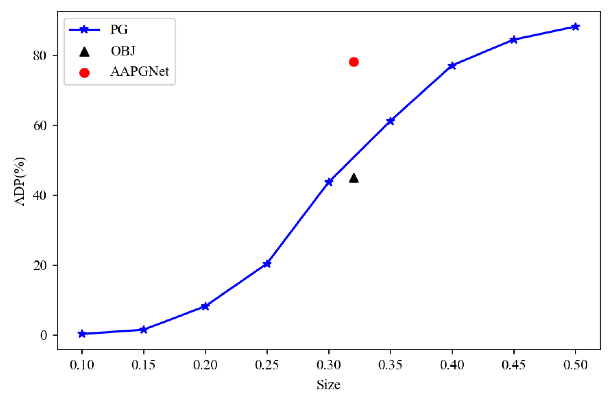
3.3. Evaluation of the Scale Adaptiveness

To evaluate the efficiency of the strategy used to increase the scale adaptiveness of our algorithm, we constructed four networks: (1) the network AAPGNet drawn in Figure 2, (2) the network without branches 2 and 3 named AAPGNet1, (3) the network without branch 3 named AAPGNet12, (4) the network without branch 2 named AAPGNet13. We also split the objects in the test dataset into two groups: (1) the objects with a size smaller than 50 × 50 pixels, and (2) the objects with a size bigger than 50 × 50 pixels. We tested these four networks on the testing dataset and separately counted the detection results on these two groups of objects. The results are listed in Table 1.
Table 1 shows that the network with three branches has the highest APD, and the network with only one branch has the lowest APD. The gap is more prominent on small objects, which means that the network with three branches has more adaptiveness to small-sized objects. That is because of the down-sampling operation, and the deep network structure makes the network lose fine-grained information about the objects, making the network ignore small objects. The three-branched network fuses different scaled feature information to obtain semantic and fine-grained information about the objects. However, the other three networks do not have sufficient fine-grained information about the objects.

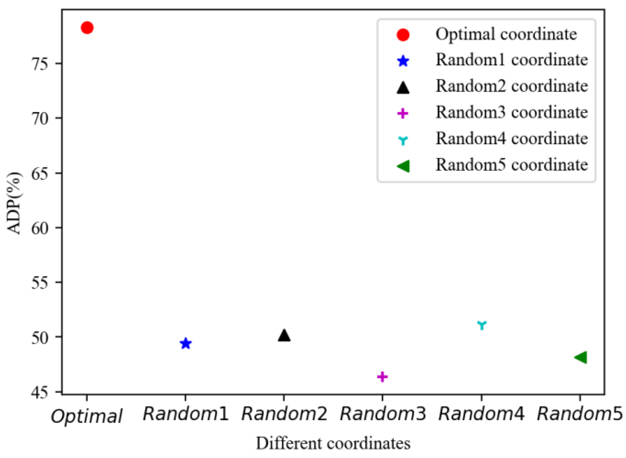
3.4. Evaluation of the Optimal Coordinate

We construct five training datasets labeled with five different patch coordinates on objects to verify the optimal patch coordinate. The five datasets are identical except for the coordinate of the patches. In these five training datasets, only one is labeled with optimal coordinates using the method described in this paper. The others are all labeled with random coordinates on objects. After constructing the training datasets, we construct five patch-generating networks on each of these five datasets using the network in Figure 2. We tested these five networks on our testing dataset and presented the results in Figure 6.
Figure 6 shows that the network trained on the dataset with optimal patch coordinates has the highest ADP, demonstrating that the optimal coordinates of patches are much better than random coordinates. This is because we are labeling the objects with patch coordinates that affect the objectness most, and detecting results of the object detection network mainly rely on the objectness.

3.5. The Influence of Different Patch Shapes

The shape of patches can affect the performance of the patch. To verify this, we generated adversarial patches with various shapes for the testing dataset, including rectangles, squares, ellipses, and circles. In the case of the ellipse, we set two axes as h/2 and w/2. For the square, we set the length of the side as k × min(h, w), and for the circle, we set the radius as k × 1/2 min(h, w). It is worth noting that when searching for the optimal patch coordinates (or optimal patch size), the shape of the noise-through window (or patch) needs to be adjusted to the corresponding shape. We recorded the results in Table 2.
Table 2 indicates that the highest APD is achieved when the patch shape is square, but the patch size is larger than other shapes and may exceed the target boundary. In terms of patch size, the elliptical patch has the smallest size, but the success rate of APD is the lowest, although it is only slightly different from that of the rectangular patch. If we use “APD/patch size” as the measure of patch deception efficiency, then the order of efficiency for several shapes is elliptical > rectangular > circle > square.

3.6. The Relationship between Patch Size and the Patch’s Adversarial Ability

In Section The Optimal Size of the Patches, we mentioned that if the patch size is too large, it will lose the adversarial ability. Generally, the bigger the patch’s size, the weaker the adversarial ability. To prove this conclusion, we designed an experiment. We used the GAN network structure drawn in Figure 4 to train two patching image-generating models. The first one was trained with 0.6 w × 0.6 h sized patches on the object’s center point, named 0.6p-net. The second one was trained with 0.4 w × 0.4 h sized patches on the object’s center point, named 0.4p-net. Afterward, (1) we patched each object in the test dataset with a 0.4 w × 0.4 h ( 0.6 w × 0.6 h ) sized patch using the patching image the 0.6p-net (0.4p-net) generated. The w and h are the width and height of the object, respectively. We recorded the APD in Table 3.
In this experiment, when training the patching image-generating models, we uncovered corresponding sized patches, for example 0.4 w × 0.4 h , from the patching image on the point corresponding to the object’s center point from the patching image. Table 3 shows a significant decline in APD when decreasing the patch size of 0.6p-net but not a considerable increase when increasing the patch size of 0.4p-net. This phenomenon indicates that the patching image generated by 0.6p-net has a weaker adversarial ability than the one generated by 0.4p-net.

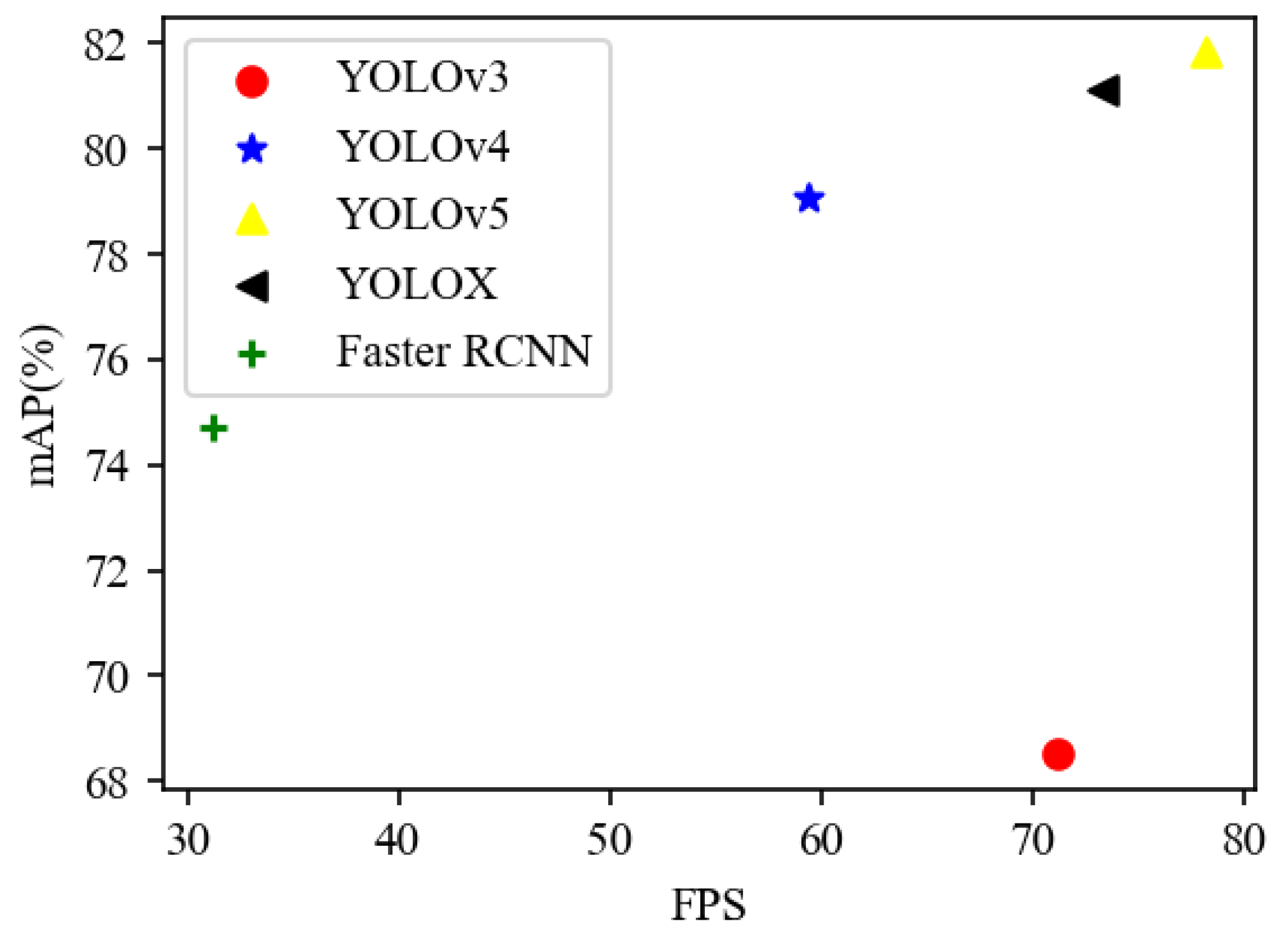
3.7. Evaluation of the Transferability

Our attacking algorithm is implemented on YOLOv5 object detection networks. We needed to test its attacking transferability to other object detection networks. Therefore, we chose Faster RCNN, YOLOv3, YOLOv4, YOLOv5, and YOLOX five networks to test the attacking transferability. During the test, we separately trained five networks on our training datasets and generate the adversarial patches on the test dataset only for YOLOv5. We used this patched testing dataset to attack four other object detection networks. The results are listed in Table 4.
Table 4 shows that our attacking algorithm can attack the YOLO type one-stage algorithm and the Faster RCNN two-stage algorithm with only one model. Our attacking algorithm is designed for YOLO type (one-stage algorithm) object detection network. However, it has transferability to the two-stage object detection network. That is because we trained our attacking model on the whole training dataset, which makes the model learn the common features of the training dataset. Therefore, if the object detection network is construed based on this training dataset, there will be a high probability that the object detection network can be attacked by the attack model trained on this dataset for other object detection networks.

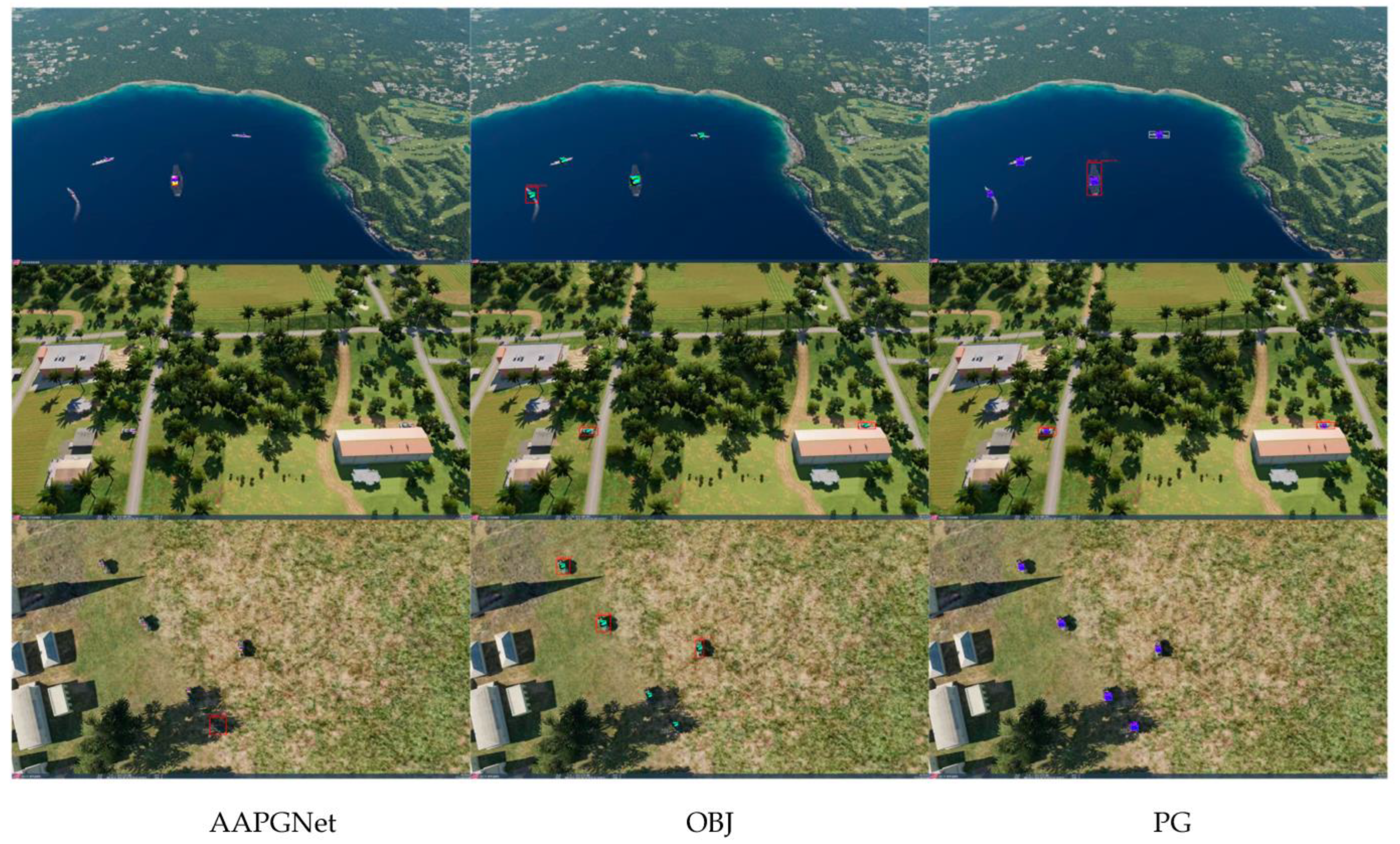
3.8. Comparing with Other Attacking Algorithms

To compare our algorithm with other adversarial patch-generating algorithms, we implemented two other patch-generating algorithms, i.e., OBJ in paper [52] and the algorithm in paper [54] (for convenience, we named it PG in this paper). For fairness, we removed the printable loss in algorithm OBJ and PG during the comparison. We set the parameters a, α , and β in PG to 0.125, 0.6, and 0.4, respectively. We recorded the average size of the patches on all objects as the size of our algorithm in Figure 7, and set the patching size of the OBJ to the size of our algorithm’s average size. The testing results are shown in Figure 7.
In Figure 7, the size represents the proportion of the patch size to the object size. Our algorithm gets the highest ADP when the size is equal to the other two algorithms, indicating that our attacking algorithm is more efficient in hiding the object from ILSST.
There is something that should be noticed. In this test, the other two algorithms needed to provide the ground truth about objects when patching the patch on each object, but our algorithm does not need the ground truth about the objects. We also visualized some of the testing results in Figure 8. In the third column of Figure 8, some patches exceed the objects, which is hard to realize in a real-world situation. In the second column of Figure 8, several ground units failed to be hidden from the detector. However, in the first column of Figure 8, not only did the patch not exceed the objects, but it also deceived the detector, which indicates that our algorithm is more efficient when hiding the object from the detector.

4. Discussion

In this paper, we presented an adaptive adversarial patch generation algorithm designed to protect military ground units from ILSST attacks or reconnaissance. In the design process, we considered the target characteristics (multiple scales) of LSST and devised an adaptive adversarial patch-generating network. During the adversarial patch generation, the network extracted features from three scales. Based on these three scaled features, an adversarial image generator was employed to produce an adversarial image, while a patching information generator predicted the positions and sizes of the patch across the three scales. Finally, based on its position and size information, we located the corresponding patch in the adversarial image and patched it onto the target. To verify the effectiveness of the multi-scale feature extraction network, we conducted ablation experiments in the experimental section. The results confirmed the efficiency of our algorithm.
Previous adversarial patch-generating algorithms generated adversarial patches by manually specifying their position and size, which is inefficient in deceiving target detection algorithms. To deal with this issue, we used the least squares method and binary search to find the optimal patch position and size for the targets in the training dataset and trained the patch generation network using this position and size information. We conducted several experiments to verify the patch’s efficiency. The results demonstrate that our algorithm can generate optimal-sized adversarial patches for targets at different positions, greatly improving the adversarial efficiency of the patches.
There is something we noticed in our experiments. The patch-generating algorithm in this paper generates patches for multiple objects in the input image, and these objects can belong to different classes. Intuitively, the patches that hide the object from the object detection network should have different color patterns. However, we found that the color patterns of the patches are surprisingly similar. We speculated that it is because the object detection networks detect all the objects as one class, i.e., the objectness class, when it discerns the object from the background. The pass-through of the same class label is consistent, which led to the noise patterns that interfere with prediction results for the same object class being similar.
The adversarial patches are needed to be transferred to real-world military units. Currently, researchers are using the non-printable loss [66] when training the patch to transfer the electronic patch to the real world. The transformation also needs the patch to be smoothly colored. The smooth color process can be achieved by using the total variation loss to restrict the frequent abrupt change of colors which is already used in our paper (mentioned in Section 3.2). However, this process will significantly reduce the adversarial effectiveness of the patch, and further extensive studies are needed to address this issue.

5. Conclusions

In this paper, we proposed an ILSST defending strategy to hide the object from the ILSST’s onboard object detection networks. The patch-generating algorithm proposed in this paper can automatically generate patches on the objects with optimal coordinates and size without the ground truth. When constructing the patch-generating network, we also considered that the ground units have an extensive range of scales from the ILSST’s view. In the end, extensive experiments are applied, and the performance of the proposed algorithm is verified. The result shows that our algorithm can effectively generate patches on objects without ground truth, has high transferability to other object detection networks, and is more effective than other similar state-of-the-art algorithms.
Currently, we have mainly verified the feasibility of our proposed defending algorithm in the simulation environment. It requires further work to establish a real-world environment and transfer the patches to real-world ground units, which requires considering clouds, light conditions, etc. In future work, we will focus on establishing real-world environments and transferring the patches to real-world ground units.

Author Contributions

Conceptualization, J.R. and Y.X.; methodology, J.R.; software, Z.Z.; validation, L.D., F.Z., T.H. and Z.Z.; formal analysis, W.F.; investigation, Z.Z.; resources, Y.X.; data curation, F.Z.; writing—original draft preparation, J.R.; writing—review and editing, C.T.; visualization, C.T.; supervision, Y.X.; project administration, Y.X.; funding acquisition, Z.Z. All authors have read and agreed to the published version of the manuscript.

Funding

This research was funded by The Nature Science Foundation of Shaanxi [grant number 2022JQ-653]; The Fundamental Research Funds for the Central Universities, Northwestern Polytechnical University [grant number D5000210767].

Data Availability Statement

The data presented in this study are available on request from the corresponding author. The data are not publicly available due to some interest issues.

Conflicts of Interest

The authors declare no conflict of interest.

References

  1. Zhang, X.; Lu, S.; Sun, J.; Shangguan, W. Low-Altitude and Slow-Speed Small Target Detection Based on Spectrum Zoom Processing. Math. Probl. Eng. 2018, 2018, 4146212. [Google Scholar] [CrossRef] [Green Version]
  2. Valenti, F.; Giaquinto, D.; Musto, L.; Zinelli, A.; Bertozzi, M.; Broggi, A. Enabling computer vision-based autonomous navigation for Unmanned Aerial Vehicles in cluttered GPS-denied environments. In Proceedings of the 2018 21st International Conference on Intelligent Transportation Systems (ITSC), Maui, HI, USA, 4–7 November 2018; IEEE: New York, NY, USA; pp. 3886–3891. [Google Scholar]
  3. Hameed, S.; Junejo, F.; Zai, M.A.Y.; Amin, I. Prediction of Civilians Killing in the Upcoming Drone Attack. In Proceedings of the 2018 IEEE 5th International Conference on Engineering Technologies and Applied Sciences (ICETAS), Bangkok, Thailand, 22–23 November 2018; pp. 1–5. [Google Scholar]
  4. Heubl, B. Consumer drones used in bomb attacks: Terrorist rebels are turning consumer drones into deadly weapons. E&T investigates why it goes on and what can be done about it. Eng. Technol. 2021, 16, 1–9. [Google Scholar]
  5. Björklund, S. Target detection and classification of small drones by boosting on radar micro-Doppler. In Proceedings of the 2018 15th European Radar Conference (EuRAD), Madrid, Spain, 26–28 September 2018; pp. 182–185. [Google Scholar]
  6. Semkin, V.; Yin, M.; Hu, Y.; Mezzavilla, M.; Rangan, S. Drone detection and classification based on radar cross section signatures. In Proceedings of the 2020 International Symposium on Antennas and Propagation (ISAP), Osaka, Japan, 25–28 January 2020; pp. 223–224. [Google Scholar]
  7. Al-Emadi, S.; Al-Ali, A.; Al-Ali, A. Audio-Based Drone Detection and Identification Using Deep Learning Techniques with Dataset Enhancement through Generative Adversarial Networks. Sensors 2021, 21, 4953. [Google Scholar] [CrossRef] [PubMed]
  8. Wang, L.; Cavallaro, A. Acoustic sensing from a multi-rotor drone. IEEE Sens. J. 2018, 18, 4570–4582. [Google Scholar] [CrossRef]
  9. Sie, N.J.; Srigrarom, S.; Huang, S. Field test validations of vision-based multi-camera multi-drone tracking and 3D localizing with concurrent camera pose estimation. In Proceedings of the 2021 6th International Conference on Control and Robotics Engineering (ICCRE), Beijing, China, 16–18 April 2021; pp. 139–144. [Google Scholar]
  10. Singha, S.; Aydin, B. Automated Drone Detection Using YOLOv4. Drones 2021, 5, 95. [Google Scholar] [CrossRef]
  11. Ezuma, M.; Erden, F.; Anjinappa, C.K.; Ozdemir, O.; Guvenc, I. Micro-UAV detection and classification from RF fingerprints using machine learning techniques. In Proceedings of the 2019 IEEE Aerospace Conference, Big Sky, MT, USA, 2–9 March 2019; pp. 1–13. [Google Scholar]
  12. Nie, W.; Han, Z.-C.; Li, Y.; He, W.; Xie, L.-B.; Yang, X.-L.; Zhou, M. UAV Detection and Localization Based on Multi-dimensional Signal Features. IEEE Sens. J. 2021, 22, 5150–5162. [Google Scholar] [CrossRef]
  13. Hoffmann, F.; Ritchie, M.; Fioranelli, F.; Charlish, A.; Griffiths, H. Micro-Doppler based detection and tracking of UAVs with multistatic radar. In Proceedings of the 2016 IEEE radar conference (RadarConf), Philadelphia, PA, USA, 2–6 May 2016; pp. 1–6. [Google Scholar]
  14. Kang, B.; Ahn, H.; Choo, H. A software platform for noise reduction in sound sensor equipped drones. IEEE Sens. J. 2019, 19, 10121–10130. [Google Scholar] [CrossRef]
  15. Zhang, Z.; Cao, Y.; Ding, M.; Zhuang, L.; Yao, W. An intruder detection algorithm for vision based sense and avoid system. In Proceedings of the 2016 International Conference on Unmanned Aircraft Systems (ICUAS), Arlington, VA, USA, 7–10 June 2016; pp. 550–556. [Google Scholar]
  16. Ganti, S.R.; Kim, Y. Implementation of detection and tracking mechanism for small UAS. In Proceedings of the 2016 International Conference on Unmanned Aircraft Systems (ICUAS), Arlington, VA, USA, 7–10 June 2016; pp. 1254–1260. [Google Scholar]
  17. Flak, P. Drone Detection Sensor with Continuous 2.4 GHz ISM Band Coverage Based on Cost-Effective SDR Platform. IEEE Access 2021, 9, 114574–114586. [Google Scholar] [CrossRef]
  18. Kim, M.; Lee, J. Impact of an interfering node on unmanned aerial vehicle communications. IEEE Trans. Veh. Technol. 2019, 68, 12150–12163. [Google Scholar] [CrossRef] [Green Version]
  19. Shepard, D.P.; Bhatti, J.A.; Humphreys, T.E. Drone hack: Spoofing attack demonstration on a civilian unmanned aerial vehicle. 2012. Available online: https://www.gpsworld.com/drone-hack/ (accessed on 3 November 2022).
  20. Glenn, J. Ultralytics/Yolov5: V6.0. 2021. Available online: https://github.com/ultralytics/yolov5 (accessed on 12 June 2022).
  21. Xu, Y.; Bai, T.; Yu, W.; Chang, S.; Atkinson, P.M.; Ghamisi, P. AI Security for Geoscience and Remote Sensing: Challenges and Future Trends. arXiv 2022, arXiv:2212.09360. [Google Scholar]
  22. Szegedy, C.; Zaremba, W.; Sutskever, I.; Bruna, J.; Erhan, D.; Goodfellow, I.; Fergus, R. Intriguing properties of neural networks. arXiv 2013, arXiv:1312.6199. [Google Scholar]
  23. Goodfellow, I.J.; Shlens, J.; Szegedy, C. Explaining and harnessing adversarial examples. arXiv 2014, arXiv:1412.6572. [Google Scholar]
  24. Kurakin, A.; Goodfellow, I.J.; Bengio, S. Adversarial examples in the physical world. In Artificial Intelligence Safety and Security; Chapman and Hall/CRC: Boca Raton, FL, USA, 2018; pp. 99–112. [Google Scholar]
  25. Dong, Y.; Liao, F.; Pang, T.; Su, H.; Zhu, J.; Hu, X.; Li, J. Boosting adversarial attacks with momentum. In Proceedings of the IEEE Conference on Computer Vision and Pattern Recognition, Salt Lake City, UT, USA, 18–23 June 2018. [Google Scholar]
  26. Moosavi-Dezfooli, S.-M.; Fawzi, A.; Frossard, P. Deepfool: A simple and accurate method to fool deep neural networks. In Proceedings of the IEEE Conference on Computer Vision and Pattern Recognition, Las Vegas, NV, USA, 27–30 June 2016; pp. 2574–2582. [Google Scholar]
  27. Papernot, N.; McDaniel, P.; Jha, S.; Fredrikson, M.; Celik, Z.B.; Swami, A. The limitations of deep learning in adversarial settings. In Proceedings of the 2016 IEEE European Symposium on Security and Privacy (EuroS&P), Saarbrucken, Germany, 21–24 March 2019; pp. 372–387. [Google Scholar]
  28. Carlini, N.; Wagner, D. Towards evaluating the robustness of neural networks. In Proceedings of the 2017 IEEE Symposium on Security and Privacy (SP), San Jose, CA, USA, 22–24 May 2017; pp. 39–57. [Google Scholar]
  29. Rony, J.; Hafemann, L.G.; Oliveira, L.S.; Ayed, I.B.; Sabourin, R.; Granger, E. Decoupling direction and norm for efficient gradient-based l2 adversarial attacks and defenses. In Proceedings of the IEEE/CVF Conference on Computer Vision and Pattern Recognition, Long Beach, CA, USA, 15–20 June 2019. [Google Scholar]
  30. Croce, F.; Hein, M. Reliable evaluation of adversarial robustness with an ensemble of diverse parameter-free attacks. In Proceedings of the International Conference on Machine Learning, Virtual, 13–18 July 2020; pp. 2206–2216. [Google Scholar]
  31. Xiao, C.; Li, B.; Zhu, J.-Y.; He, W.; Liu, M.; Song, D. Generating adversarial examples with adversarial networks. arXiv 2018, arXiv:1801.02610. [Google Scholar]
  32. Bai, T.; Zhao, J.; Zhu, J.; Han, S.; Chen, J.; Li, B.; Kot, A. Ai-gan: Attack-inspired generation of adversarial examples. In Proceedings of the 2021 IEEE International Conference on Image Processing (ICIP), Anchorage, AK, USA, 19–22 September 2021; pp. 2543–2547. [Google Scholar]
  33. Xie, C.; Wang, J.; Zhang, Z.; Zhou, Y.; Xie, L.; Yuille, A. Adversarial Examples for Semantic Segmentation and Object Detection. In Proceedings of the 2017 IEEE International Conference on Computer Vision (ICCV), Venice, Italy, 22–29 October 2017; pp. 1378–1387. [Google Scholar]
  34. Li, Y.; Tian, D.; Chang, M.-C.; Bian, X.; Lyu, S. Robust adversarial perturbation on deep proposal-based models. arXiv 2018, arXiv:1809.05962. [Google Scholar]
  35. Wei, X.; Liang, S.; Chen, N.; Cao, X. Transferable adversarial attacks for image and video object detection. arXiv 2018, arXiv:1811.12641. [Google Scholar]
  36. Goodfellow, I.; Pouget-Abadie, J.; Mirza, M.; Xu, B.; Warde-Farley, D.; Ozair, S.; Courville, A.; Bengio, Y. Generative adversarial networks. Commun. ACM 2020, 63, 139–144. [Google Scholar] [CrossRef]
  37. Athalye, A.; Engstrom, L.; Ilyas, A.; Kwok, K. Synthesizing Robust Adversarial Examples. In Proceedings of the International Conference on Machine Learning, Stockholm, Sweden, 10–15 July 2018; Volume 80. [Google Scholar]
  38. Wang, D.; Li, C.; Wen, S.; Han, Q.L.; Nepal, S.; Zhang, X.; Xiang, Y. Daedalus: Breaking Nonmaximum Suppression in Object Detection via Adversarial Examples. IEEE Trans. Cybern. 2022, 52, 7427–7440. [Google Scholar] [CrossRef]
  39. Brown, T.B.; Mané, D.; Roy, A.; Abadi, M.; Gilmer, J. Adversarial patch. arXiv 2017, arXiv:1712.09665. [Google Scholar]
  40. Karmon, D.; Zoran, D.; Goldberg, Y. Lavan: Localized and visible adversarial noise. In Proceedings of the International Conference on Machine Learning, Stockholm, Sweden, 10–15 July 2018. [Google Scholar]
  41. Chindaudom, A.; Siritanawan, P.; Sumongkayothin, K.; Kotani, K. AdversarialQR: An adversarial patch in QR code format. In Proceedings of the 2020 Joint 9th International Conference on Informatics, Electronics & Vision (ICIEV) and 2020 4th International Conference on Imaging, Vision & Pattern Recognition (icIVPR), Kitakyushu, Japan, 26–29 August 2020; pp. 1–6. [Google Scholar]
  42. Chindaudom, A.; Siritanawan, P.; Sumongkayothin, K.; Kotani, K. Surreptitious Adversarial Examples through Functioning QR Code. J. Imaging 2022, 8, 122. [Google Scholar] [CrossRef]
  43. Gittings, T.; Schneider, S.; Collomosse, J. Robust synthesis of adversarial visual examples using a deep image prior. arXiv 2019, arXiv:1907.01996. [Google Scholar]
  44. Zhou, X.; Pan, Z.; Duan, Y.; Zhang, J.; Wang, S. A data independent approach to generate adversarial patches. Mach. Vis. Appl. 2021, 32, 1–9. [Google Scholar] [CrossRef]
  45. Bai, T.; Luo, J.; Zhao, J. Inconspicuous adversarial patches for fooling image-recognition systems on mobile devices. IEEE Internet Things J. 2021, 9, 9515–9524. [Google Scholar] [CrossRef]
  46. Song, D.; Eykholt, K.; Evtimov, I.; Fernandes, E.; Li, B.; Rahmati, A.; Tramer, F.; Prakash, A.; Kohno, T. Physical adversarial examples for object detectors. In Proceedings of the 12th USENIX Workshop on Offensive Technologies (WOOT 18), Baltimore, MD, USA, 13–14 August 2018. [Google Scholar]
  47. Eykholt, K.; Evtimov, I.; Fernandes, E.; Li, B.; Rahmati, A.; Xiao, C.; Prakash, A.; Kohno, T.; Song, D. Robust physical-world attacks on deep learning visual classification. In Proceedings of the IEEE Conference on Computer Vision and Pattern Recognition, Salt Lake City, UT, USA, 18–23 June 2018; pp. 1625–1634. [Google Scholar]
  48. Ren, S.; He, K.; Girshick, R.; Sun, J. Faster r-cnn: Towards real-time object detection with region proposal networks. arXiv 2015, arXiv:1506.01497. [Google Scholar] [CrossRef] [PubMed] [Green Version]
  49. Bochkovskiy, A.; Wang, C.-Y.; Liao, H.-Y.M. Yolov4: Optimal speed and accuracy of object detection. arXiv 2020, arXiv:2004.10934. [Google Scholar]
  50. Wu, S.; Dai, T.; Xia, S.-T. Dpattack: Diffused patch attacks against universal object detection. arXiv 2020, arXiv:2010.11679. [Google Scholar]
  51. Lee, M.; Kolter, Z. On physical adversarial patches for object detection. arXiv 2019, arXiv:1906.11897. [Google Scholar]
  52. Thys, S.; Van Ranst, W.; Goedemé, T. Fooling automated surveillance cameras: Adversarial patches to attack person detection. In Proceedings of the IEEE/CVF Conference on Computer Vision and Pattern Recognition Workshops, Long Beach, CA, USA, 16–17 June 2019. [Google Scholar]
  53. Komkov, S.; Petiushko, A. AdvHat: Real-World Adversarial Attack on ArcFace Face ID System. In Proceedings of the 2020 25th International Conference on Pattern Recognition (ICPR), Milan, Italy, 10–15 January 2021; pp. 819–826. [Google Scholar]
  54. Wang, Y.; Lv, H.; Kuang, X.; Zhao, G.; Tan, Y.-a.; Zhang, Q.; Hu, J. Towards a physical-world adversarial patch for blinding object detection models. Inf. Sci. 2021, 556, 459–471. [Google Scholar] [CrossRef]
  55. Czaja, W.; Fendley, N.; Pekala, M.; Ratto, C.; Wang, I.-J. Adversarial examples in remote sensing. In Proceedings of the 26th ACM SIGSPATIAL International Conference on Advances in Geographic Information Systems, Seattle, DC, USA, 6–9 November 2019; pp. 408–411. [Google Scholar]
  56. Chen, L.; Zhu, G.; Li, Q.; Li, H. Adversarial example in remote sensing image recognition. arXiv 2019, arXiv:1910.13222. [Google Scholar]
  57. Xu, Y.; Ghamisi, P. Universal adversarial examples in remote sensing: Methodology and benchmark. IEEE Trans. Geosci. Remote Sens. 2022, 60, 1–15. [Google Scholar] [CrossRef]
  58. Zhang, Y.; Zhang, Y.; Qi, J.; Bin, K.; Wen, H.; Tong, X.; Zhong, P. Adversarial Patch Attack on Multi-Scale Object Detection for UAV Remote Sensing Images. Remote Sens. 2022, 14, 5298. [Google Scholar] [CrossRef]
  59. Bai, T.; Wang, H.; Wen, B. Targeted Universal Adversarial Examples for Remote Sensing. Remote Sens. 2022, 14, 5833. [Google Scholar] [CrossRef]
  60. Shi, C.; Dang, Y.; Fang, L.; Lv, Z.; Zhao, M. Hyperspectral image classification with adversarial attack. IEEE Geosci. Remote Sens. Lett. 2021, 19, 1–5. [Google Scholar] [CrossRef]
  61. Chen, L.; Xu, Z.; Li, Q.; Peng, J.; Wang, S.; Li, H. An empirical study of adversarial examples on remote sensing image scene classification. IEEE Trans. Geosci. Remote Sens. 2021, 59, 7419–7433. [Google Scholar] [CrossRef]
  62. Li, H.; Huang, H.; Chen, L.; Peng, J.; Huang, H.; Cui, Z.; Mei, X.; Wu, G. Adversarial examples for CNN-based SAR image classification: An experience study. IEEE J. Sel. Top. Appl. Earth Obs. Remote Sens. 2020, 14, 1333–1347. [Google Scholar] [CrossRef]
  63. Zheng, Z.; Wang, P.; Liu, W.; Li, J.; Ye, R.; Ren, D. Distance-IoU loss: Faster and better learning for bounding box regression. In Proceedings of the Thirty-Fourth AAAI Conference on Artificial Intelligence, New York, New York, USA, 7–12 February 2020. [Google Scholar]
  64. Redmon, J.; Farhadi, A. Yolov3: An incremental improvement. arXiv 2018, arXiv:1804.02767. [Google Scholar]
  65. Ge, Z.; Liu, S.; Wang, F.; Li, Z.; Sun, J. Yolox: Exceeding yolo series in 2021. arXiv 2021, arXiv:2107.08430. [Google Scholar]
  66. Sharif, M.; Bhagavatula, S.; Bauer, L.; Reiter, M.K. Accessorize to a crime: Real and stealthy attacks on state-of-the-art face recognition. In Proceedings of the 2016 Acm Sigsac Conference on Computer and Communications Security, Vienna, Austria, 24–28 October 2016; pp. 1528–1540. [Google Scholar]
Figure 1. The structure of our algorithm. The upper part is the data labeling process which labels the objects in the dataset with the optimal location and size of the patch. The lower part is the patch-generating network which uses the labeled dataset to train a model that can generate a patching image and a mask for an input image. The mask is used to select the areas from the patching image and patch the selected areas to the objects.
Remotesensing 15 01439 g001
Figure 2. Adaptive adversarial patch-generating network. The main structure of the network consists of three parts, (1) the backbone used to extract features from the input; (2) the patching image generator that uses the features extracted by the backbone to generate a patching image with a size identical to the input image; (3) the patching information generator that uses the features extracted by backbone to generate mask on the patching location. Finally, the mask on the patching image is used to select the corresponding patch out from the patching image and patch it on the objects. The red circled numbers represent different scaled branches for ablation experiments in Section 3.3.
Remotesensing 15 01439 g002
Figure 3. DeFOCUS. The DeFOCUS can transform every four adjacent channels of the input layer as one channel of the output layer and enlarge the size of the input layer by two. In this figure, we used different colors to indicate channels of the feature map that needs to be enlarged by two.
Remotesensing 15 01439 g003
Figure 4. Adversarial noise-generating network. The main structure of the network is similar to the network of backbone plus patching image generator in Figure 2. The CBS, DCBS, and CSP modules are the same as those in Figure 2.
Remotesensing 15 01439 g004
Figure 5. Performance comparison of multiple target detection networks. The horizontal axis FPS is the abbreviation of the frames per second, which indicate the operating speed of the algorithms.
Remotesensing 15 01439 g005
Figure 6. Comparison of the different patch’s coordinates. The “Random n” in the horizontal axis represents datasets labeled with different random coordinates, and “Optimal” represents the dataset labeled using our algorithm.
Remotesensing 15 01439 g006
Figure 7. Performance comparison of the attacking algorithms. In this figure, for PG algorithm, we varied the patch size from 0.1 to 0.5 in the paper and presented it as a reference for readers.
Remotesensing 15 01439 g007
Figure 8. Visualized results of different attacking algorithms. The red box is the object’s bounding box, and the letters and the number on the top of the red box are the class name and the objectness.
Remotesensing 15 01439 g008
Table 1. Testing result of the scale adaptiveness.
DatasetmAPbAttack AlgorithmsmAPaAPD
Small objects74.11%AAPGNet21.57%70.90%
AAPGNet140.99%44.69%
AAPGNet1229.28%60.49%
AAPGNet1324.60%66.80%
Large objects89.57%AAPGNet13.74%84.66%
AAPGNet134.58%61.39%
AAPGNet1224.22%72.96%
AAPGNet1325.72%71.29%
Table 2. Comparison of the different-shaped patches.
ShapemAPbmAPaAPDAverage Size
Rectangle81.84%17.8%78.25%0.32
Square15.86%80.62%0.41
Elliptical18.49%77.4%0.27
Circle16.43%79.92%0.35
Table 3. Comparison of the different-sized patches.
Control GroupmAPbmAPaAPD
0.6p-net with 0.6 w × 0.6 h sized patch 81.84%10.04%87.73%
0.4p-net with 0.4 w × 0.4 h sized patch81.84%30.62%62.59%
0.6p-net with 0.4 w × 0.4 h sized patch81.84%53.55%34.57%
0.4p-net with 0.6 w × 0.6 h sized patch81.84%28.36%65.35%
Table 4. Transferability testing results.
AlgorithmmAPb mAPaAPD
YOLOv581.84%17.8%78.25%
Faster RCNN74.59%22.95%69.23%
YOLOv368.52%15.48%77.41%
YOLOv479.06%21.13%73.27%
YOLOX81.13%23.5%71.03%
Disclaimer/Publisher’s Note: The statements, opinions and data contained in all publications are solely those of the individual author(s) and contributor(s) and not of MDPI and/or the editor(s). MDPI and/or the editor(s) disclaim responsibility for any injury to people or property resulting from any ideas, methods, instructions or products referred to in the content.

