A Bibliometric and Visualized Analysis of Remote Sensing Methods for Glacier Mass Balance Research

Abstract

In recent decades, climate change has led to global warming, glacier melting, glacial lake outbursts, sea level rising, and more extreme weather, and has seriously affected human life. Remote sensing technology has advanced quickly, and it offers effective observation techniques for studying and monitoring glaciers. In order to clarify the stage of research development, research hotspots, research frontiers, and limitations and challenges in glacier mass balance based on remote sensing technology, we used the tools of bibliometrics and data visualization to analyze 4817 works of literature related to glacier mass balance based on remote sensing technology from 1990 to 2021 in the Web of Science database. The results showed that (1) China and the United States are the major countries in the study of glacier mass balance based on remote sensing technology. (2) The Chinese Academy of Sciences is the most productive research institution. (3) Current research hotspots focus on “Climate change”, “Inventory”, “Dynamics”, “Model”, “Retreat”, “Glacier mass balance”, “Sea level”, “Radar”, “Volume change”, “Surface velocity”, “Glacier mapping”, “Hazard”, and other keywords. (4) The current research frontiers include water storage change, artificial intelligence, High Mountain Asia (HMA), photogrammetry, debris cover, geodetic method, area change, glacier volume, classification, satellite gravimetry, grounding line retreat, risk assessment, lake outburst flood, glacier elevation change, digital elevation model, geodetic mass balance, (DEM) generation, etc. According to the results of the visual analysis of the literature, we introduced the three commonly used methods of glacier mass balance based on remote sensing observation and summarized the research status and shortcomings of different methods in glacier mass balance. We considered that the future research trend is to improve the spatial and temporal resolution of data and combine a variety of methods and data to achieve high precision and long-term monitoring of glacier mass changes and improve the consistency of results. This research summarizes the study of glacier mass balance using remote sensing, which will provide valuable information for future research across this field.

1. Introduction

Glaciers are ice bodies that are formed over many years by the accumulation and evolution (compression, recrystallization, thawing, and refreezing) of snow or other solid precipitation, which typically move according to deformations caused by internal strain or by sliding along a bottom interface [1]. A glacier is an important indicator of climate change. Changes in glacier mass balance, terminal advance and retreat, and reserves are related to climate on different scales [2]. As a “solid reservoir”, glaciers are not only the most valuable freshwater resource in arid zones, but also the source of many important rivers, and their melting has an important impact on the ocean [3]. In recent years, under the influence of climate warming and human activities, glaciers have been melting significantly, and disasters such as glacier collapse and glacial lake outbursts have occurred frequently, affecting the life of tens of thousands of people [4]. Understanding the characteristics and trends of glacier changes and exploring the impact of glacier changes on regional natural ecology, disaster development, and climate change have become topics of great concern to the international community.

Glacier mass balance is an intuitive response of glacier mass accumulation and ablation and describes climate change in relation to glacier feedback by quantifying glacier mass changes [5]. Traditional glaciological methods are usually limited to a limited number of accessible glaciers and are difficult to carry out on a large scale in areas with a complex topography and hard environments [6]. Since the 1990s, remote sensing technology has been widely used for the dynamic monitoring of global cryosphere changes due to its comprehensive, dynamic, and rapid advantages, providing data support for glacier monitoring in hard-to-reach areas. The assessment of glacier mass balance has made great progress in the past three decades [7,8,9,10]. At present, there are three quantitative assessment methods for glacier mass balance. The first is satellite gravimetry [11,12,13,14,15,16]. Satellite gravity measures changes in the Earth’s surface or internal mass by monitoring changes in the gravitational field, so we can estimate changes in glacier mass based on changing gravity signatures [17]. Commonly used is the gravity recovery and climate explorer satellite (GRACE). The second is the geometric method [17,18,19,20,21,22]. Using a laser altimeter satellite and a radar altimeter satellite, DEM is derived from stereo images or SAR interferometry to estimate the elevation change of glaciers, which is then converted to mass change. The third is the input–output method (IOM) [23]. GPS and interferometric synthetic aperture radar (InSAR) observation methods are used to measure the difference between mass accumulation, surface sublimation, meltwater runoff, and the ice flux from glaciers into the ocean. The three methods have provided a wealth of valuable findings and insights into glacier mass change detection.

The rapidly developing remote sensing technologies (including imaging and non-imaging remote sensing) can obtain high spatial and temporal resolution and high accuracy deformation monitoring and topographic mapping results, which have unparalleled advantages over other means in glacier mass balance studies. For example, Gardelle J et al. used SPOT-5 stereo image pairs and SRTM DEM to obtain glacier mass balance results for 2000–2011 in the Pamir–Karakorum–Himalaya [24], and Brun F et al. used ASTER stereo image pair DEM to extract glacier mass balance for 2000–2016 in HMA [19]. Although many studies have been conducted, limited attention has been paid to outlining the research trends in this area [25,26,27]. Several empirical and qualitative review articles outline glacier mass balance studies based on remote sensing. However, these studies are limited in some specific aspects such as area, time, and data methodology [27,28,29]. Therefore, in order to have a comprehensive understanding of the glacier mass balance research based on remote sensing, the bibliometric visualization analysis method is adopted to sort out the current status of relevant studies and analyze their evolution, and help us obtain a general understanding of future research.

Bibliometric analysis, which is a qualitative and quantitative examination of database-indexed publications based on mathematical and statistical methodologies, may efficiently characterize the structure of knowledge, characteristics, and trends in a certain area [30]. Quantitative analysis can help researchers who are interested in the field but unfamiliar with it to quickly grasp the basic status of the field [31]. Knowledge mapping combines information visualization techniques with traditional scientometric citation analysis to visualize knowledge of a discipline or field through data mining, information processing, scientific measurement, and graphical drawing. Because the use of knowledge maps can explore the development and relationships between different pieces of scientific knowledge [32], this technique has been widely used for bibliometric analysis in various disciplines [33,34,35].

In order to provide a systematic and objective overview of remote sensing-based glacier mass balance research, this study identifies the bibliometric characteristics of the field published on the Web of Science (WoS) between 1990 and 2021 and visualizes the relationships between articles in the field through a CiteSpace-based scientometric analysis. The objectives of this study include (1) determining the trend of the number of articles and citations; (2) identifying the representative journals, countries, institutions, and authors studying this field; (3) revealing research hotspots; (4) discovering the research frontier; and (5) summarizing the development, defects, and challenges in this field.

2. Data and Methods

2.1. Data Acquisition

WoS is the world’s largest comprehensive academic information resource covering most disciplines, including more than 8700 core academic journals of the most influential research fields in natural science, engineering technology, biomedicine, and other fields. It is a web-based product developed by Thomson Scientific [36]. It is a large, comprehensive, multidisciplinary, and core periodical citation index database. These include SCIE (Science Citation Index Expanded), SSCI (Social Science Citation Index), and AHCI (Arts and Humanities Citation Index). In this paper, WoS was used as the literature search platform, and the “WoS Core Collection” database was selected for the search period of 1990–2021. We considered existing remote sensing methods utilized for monitoring glacier mass change or likely to be used in the future, so as to find all relevant literature as comprehensively as possible. TS = (“glacier change, glacier mass balance, glacier mass change, glacier area change, glacier elevation change, glacier volume change” and “SAR, Lidar, Radar, GNSS, Altimetry, Stereo imagery, satellite remote sensing, airborne remote sensing, photogrammetry, AAR, ICESAT, ICESAT- 2, ERS-1, ENVISAT, CryoSat, SRTM, Tandem-X, Aster, ZY-3, SPOT, ALOS, KH-9, Hexagon, Corona, Pleiades, AW3D30, Geoeye-1, Quickbird, optical image, DEM, RadarSat, Sentinel, TerraSAR-X, WorldView, ERS-2, laser altimetry, JASON, remote sensing, satellite image, GRACE, GRACE follow on, gravity”) were used as search criteria. The literature that was not relevant to the study topic was manually removed after the search, and the final data obtained had 4817 search records. There may still be some irrelevant or erroneous data in the retrieved data. However, the integrity of the literature search and research topics should be ensured. Meanwhile, these irrelevant retrieval data will be exposed in the subsequent analysis of the map of scientific knowledge and can be corrected in the subsequent analysis. It is also possible to make some unexpected knowledge discoveries from these unexpected data [37].

2.2. Scientometric Analytical Methods

Bibliometrics is a discipline that takes the document system and bibliometric characteristics as the research object and uses mathematical, statistical, and other quantitative research methods to study the distribution structure, quantitative relationship, change rules, and quantitative management of document information, and then discusses some structures, characteristics, and laws of science and technology [38]. Information visualization is an interdisciplinary field, which aims to study the visual presentation of large-scale non-numerical value information resources and help to understand and analyze data by graphics and images [39]. Knowledge mapping is a graphical representation that combines bibliometric methods and information visualization principles to show the evolution and structural relationships of scientific knowledge [40]. CiteSpace is a java application for literature analysis and visualization developed by Prof. Chaomei Chen of the Drexel University School of Information Science and Technology. Its main function is to present the key evolutionary paths of research fields through metrological modeling and mapping of literature related to research fields, helping users to detect research frontiers and realize the transformation of literature research from subjective fragmentation to objective panorama [37]. Based on this approach, the paper finds the key and active themes and explores the frontier and hotspots for objectively understanding the whole picture of glacier mass balance research based on remote sensing technology.

3. Results

3.1. Basic Characteristics of the Literature

The trend of the amount of academic literature in this field over time can effectively show the state of research and further predict its development trends [41]. The number of publications and citations of remote sensing-based glacier mass balance studies from 1990 to 2021 over time are shown in Figure 1. There are three stages according to the time series. From 1990 to 1996, the annual publications were less than 10 articles, indicating research in this field that was at a low level and was not sufficiently active to be taken seriously. From 1997 to 2006, the publications were between 30 and 95, and this has been increasing rapidly each year since 2007. From the overall view, the literature volume showed a near-exponential growth trend. According to Price, if the number of works in a certain research field shows an exponential growth trend, it indicates that the development trend of the field is not yet saturated, but is still in a period of rapid development where new theories, new methods, and new technologies will emerge continuously [42].

From 1990 to 2021, the total number of citations was 152,039 and the average number of citations per publication was 31.56. Figure 1 also shows the trend of citations over the last 21 years. Due to the increasing interest in climate change and the impact of glaciers on climate change, it is clear that the number of cited papers on remote sensing-based glacier mass balance studies increased from 1990 to 2021, with two significant leaps in remote sensing-based glacier mass balance studies in 2016 and 2021. These trends reflect the increasing interest in this field over the past three decades. This is related to the development of earth observation satellite technology, with more and more satellites being launched, providing a large amount of high-precision and high-resolution data to support the study of glacier mass change [43].

The results showed that 4817 articles were published in 614 journals.

Table 1. Top ten journals by the number of publications.

Top	Journals	Publications
1	Journal of Glaciology	464
2	Cryosphere	366
3	Remote Sensing	309
4	Geophysical Research Letters	178
5	Annals of Glaciology	167
6	Remote Sensing of Environment	152
7	Journal of Geophysical Research: Earth Surface	146
8	IEEE International Symposium on Geoscience and Remote Sensing (IGARSS)	127
9	Frontiers in Earth Science	106
10	Geomorphology	100

lists the top ten journals by the number of articles. In Table 1, it can be seen that the Journal of Glaciology, Cryosphere, and Remote Sensing are the journals that published more than 300 articles. These journals cover relevant publications in the fields of glaciology, remote sensing, environmental sciences, earth sciences, etc. This indicates the diverse and cross-cutting nature of remote sensing-based glacier mass balance research and reflects the systematic and complex development of this research.

Two journals being cited by the same literature is known as journal co-citation [44]. Journal co-citation analysis allows for the positioning and classification of journals and the identification of their core or marginal position in the discipline. Figure 2 displays the journal co-citation network of this research. It can be seen from

Table 2. Top 10 journals by citation.

Top	Cited Journals	Count
1	Journal of Glaciology	3463
2	Geophysical Research Letters	2857
3	Science	2771
4	Annals of Glaciology	2682
5	Cryosphere	2496
6	Remote Sensing of Environment	2249
7	Nature	2218
8	Journal of Geophysical Research: Earth Surface	1872
9	Global and Planetary Change	1757
10	Nature Geoscience	1713

, the Journal of Glaciology, Geophysical Research Letters, Science, Annals of Glaciology, Cryosphere, Remote Sensing of Environment, and Nature are the most frequently cited journals.

3.2. Research Platforms and Core Strengths

Authors and their collaborative relationships are a central element of a research field and an important indication of the strength of research in that field. The author collaboration map shows the number of publications by authors, the collaborative relationships between the different authors, and their contributions to the field of research [45].

Table 3. Top 10 authors based on frequency.

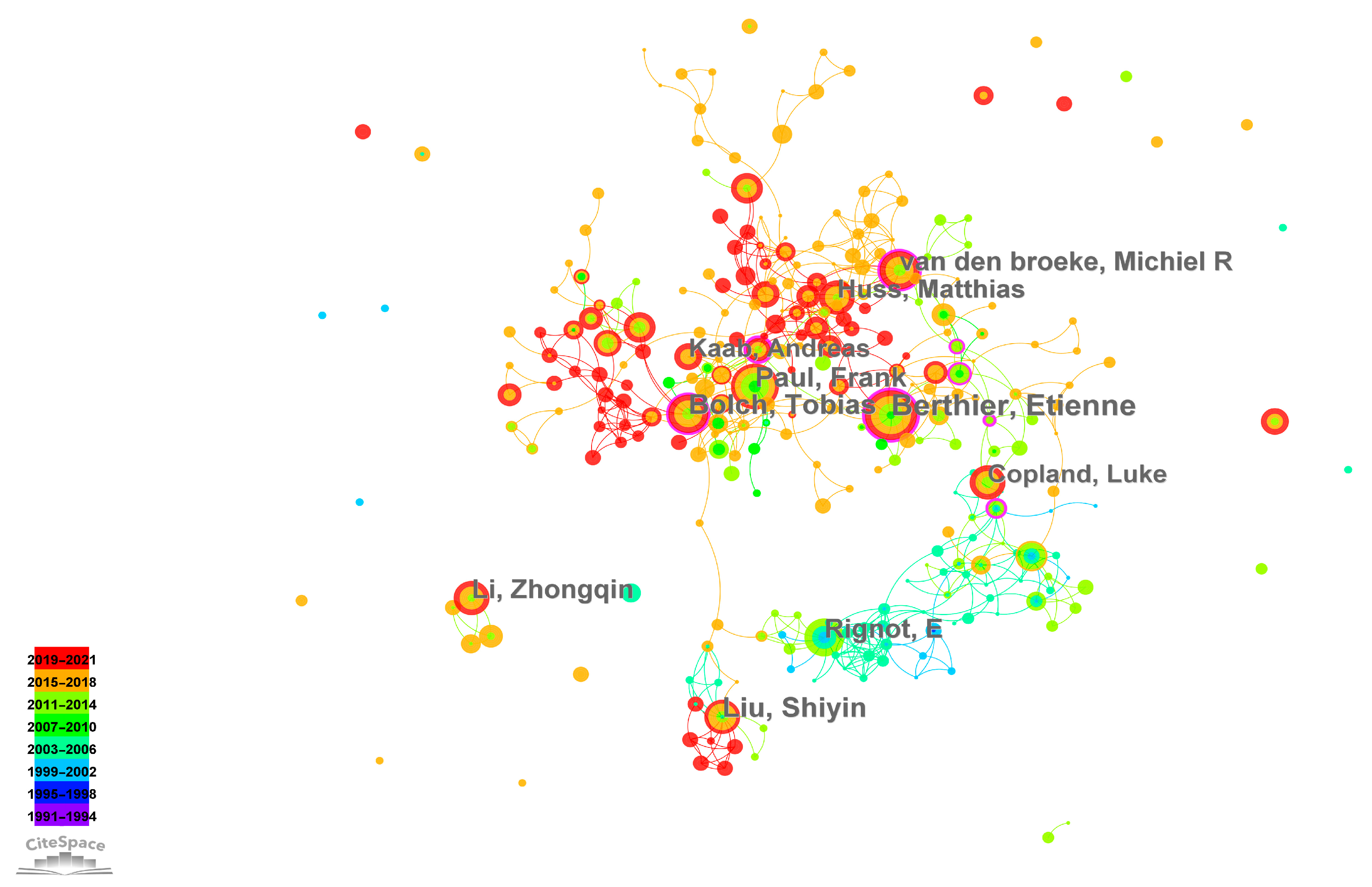
Top	Author	Freq.	Centrality
1	Berthier E	94	0.10
2	Kääb A	85	0.10
3	Liu SY	82	0.05
4	Rignot E	81	0.04
5	Bolch T	73	0.14
6	Paul F	66	0.05
7	Van den Broeke M	66	0.05
8	Kulkarni AV	56	0.00
9	Li ZQ	55	0.00
10	Huss M	50	0.00

shows the top ten most productive authors. According to the table, Berthier E and Kääb A dominate the list of publications. They are still at a high level of productivity.

Figure 3 shows a collaborative network map of remote sensing-based glacier mass balance authors consisting of 427 authors and 725 collaborative links. Figure 3 is characterized by overall dispersion and local aggregation, forming large groups represented by Berthier E, Kääb A, Bolch T, Paul F, Van den Broeke M, Huss M et al., and four small groups represented by Rignot E, Liu SY, Li ZQ, and Copland L. In terms of the scope and extent of collaboration, the authors collaborated not only within groups but also across groups. In terms of the depth of connectivity, the authors with more publications collaborate more frequently with other authors, which also indicates that inter-scholar communication has an important impact on research output. Centrality is a crucial metric used in CiteSpace to assess the significance of keywords. From the perspective of information transmission, the higher the value, the more significant the nodes are and the larger the impact on network transmission when these nodes are removed. Bolch T has the highest centrality, which means that most of the other authors’ partners met through him and acted as good intermediaries. Berthier E has the most papers. The group of authors associated with Berthier E focuses on glaciological studies using remotely sensed data [25,46,47]. His research is mainly focused on the global mass change of glaciers and their contribution to sea level rise [48,49]. In addition, he also aims to facilitate the glaciological community’s access to high-resolution satellite stereo data and DEMs [50,51,52,53,54]. The link colors are mostly green, orange, and red, indicating that most of the collaboration took place between 2014 and 2021.

The concept of co-citation analysis was first introduced by Henry Small in 1973 [56]. When two documents appear together in the reference list of a third cited document, they form a co-citation relationship. The process of mining a collection of literature for co-citation relationships is called co-citation analysis. The higher the co-citation frequency, the closer they are to each other. Through statistical methods such as cluster analysis, multidimensional scale analysis, and factor analysis, the core authors in a subject area can be classified according to this “distance” and represented graphically to visually identify and analyze the scientific community in the subject area [57].

Table 4. Top ten productive authors.

Author	Freq.	Centrality
Rignot E	1069	0.83
Kääb A	928	0.83
Bolch T	910	0.45
Paul F	847	0.50
Joughin I	605	0.28
Huss M	587	0.14
Berthier E	581	0.03
Benn DI	569	0.00
Haeberli W	568	0.41
Oerlemans J	563	0.56

lists the top 10 authors with citation frequencies above 500. It should be noted that in this analysis, only the first author is considered. Figure 4 shows the collaborative network of authors contributing to the field of glacier mass balance, which contains 427 nodes and 725 co-citation links. The most cited author was Rignot E (1069 citations), followed by Kääb A (928 citations). By comparing Table 4 to the authors listed in Table 3, we can see that Rignot E, Kääb A, Bolch T, Paul F, Berthier E, and Huss M appear in both tables, indicating that they are both the most prolific and influential authors. Rignot E is widely cited and has had a significant impact in the field, although he has published fewer papers than other authors. In the table, it can be seen that Rignot E and Kääb A have the largest centrality value, which indicates that their papers have been highly influential throughout the field of study.

The WoS database literature record contains information on the countries and institutions where the literature is published, through which the geospatial distribution of research on the topic can be characterized. Figure 5 shows that the study is predominantly spread across 118 countries worldwide, with concentrations in Europe, North America, East Asia, and South Asia.

Table 5. Top ten countries by number of articles.

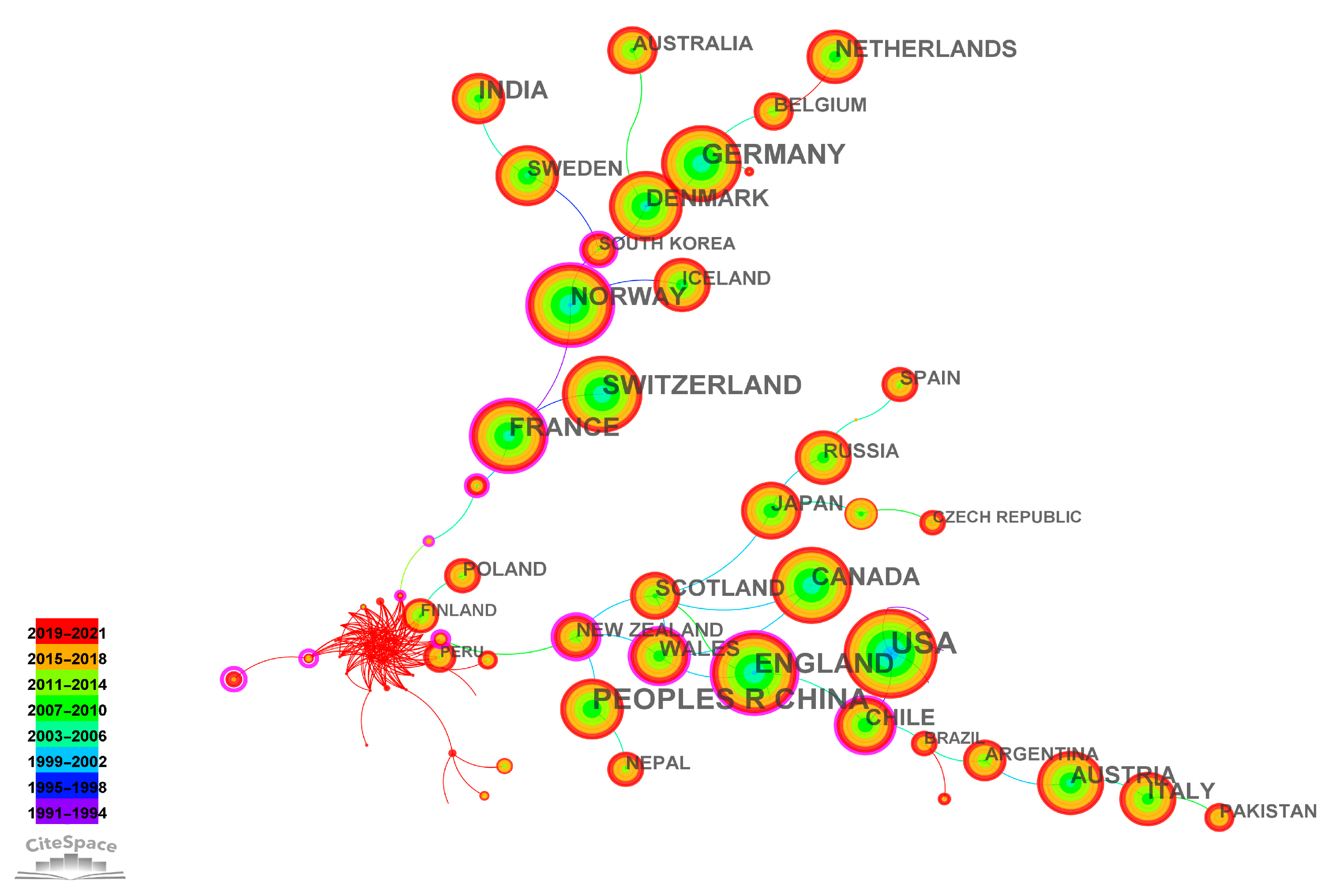
Country/Region	Freq.	Centrality
USA	1444	0.06
China	1011	0.02
England	632	0.02
Germany	601	0.25
Switzerland	506	0.02
France	450	0.05
India	389	0.02
Norway	383	0.02
Canada	354	0.02
Netherlands	255	0.00

lists the top 10 most productive countries. The United States has the most publications. This is inextricably linked to its advanced satellite technology. China has the second-highest number of publications. Glacier retreat on the Qinghai–Tibet Plateau has attracted widespread scholarly attention due to increased glacier retreat under climate warming. In addition, the public availability of high-resolution remote sensing data and the launch of the ZY-3 satellites have contributed to glaciological research [58]. The top ten countries also include England, Germany, Switzerland, France, India, Norway, Canada, and the Netherlands.

Between 1990 and 2021, the network of cooperating countries consists of 323 nodes and 1354 links (Figure 6). Obviously, there is close cooperation between the countries and regions with the most published articles. It is worth mentioning that Germany, USA, and France have a high centrality and, therefore, they play a crucial role in establishing links with other countries.

Between 1990 and 2021, the institutional collaboration network consisted of 186 institutions and 178 collaborative links, as shown in Figure 7. The relatively tight structure and close relationships indicate a relatively high level of maturity in the research community.

Table 6. Top ten institutions by number of articles.

Top	Institution	Freq.	Centrality
1	Chinese Academy of Sciences	773	0.28
2	University of Colorado	199	0.04
3	University of Zurich	175	0.08
4	California Institute of Technology	161	0.39
5	University of Oslo	143	0.09
6	NASA	142	1.02
7	Utrecht University	141	0.11
8	University Grenoble Alpes	118	0.32
9	University of Leeds	115	0.17
10	Ohio State University	113	0.09

lists the top 10 institutions that contribute the most to the total output. The Chinese Academy of Sciences tops the list with 773 publications. This also illustrates the development and advancement of China’s technical strength in the field over the years, thanks to the launch of various remote sensing satellite missions and the recognition of the importance of glacier change monitoring research. In addition, China is home to the largest mountain glacier other than the North and South Polar ice caps—the Qinghai–Tibet Glacier. In recent years, changes in Qinghai–Tibetan glaciers have become important for climate change, regional ecological changes, carbon peaking, management of surrounding water resources, and IPCC intergovernmental negotiations, and with the development of remote sensing technology, remote sensing monitoring studies of Qinghai–Tibetan glaciers have become increasingly important and numerous in China. Other institutions with a large number of publications include the University of Colorado, the University of Zurich, the California Institute of Technology, and the University of Oslo.

It can be seen that the United States is the largest contributor to remote sensing-based glacier mass balance studies with four institutions (ranked 2nd, 4th, 6th, and 10th). In addition to this, there is one institution in China (ranked first), one in Switzerland (ranked third), one in Norway (ranked fifth), one in the Netherlands (ranked seventh), one in the UK (ranked ninth), and one in France (ranked eighth). Among them, the University of Colorado has the closest cooperation with other institutions.

3.3. Research Hotspots and Research Frontiers

Citation literature analysis can study the knowledge base of the existing literature by describing the co-citation relationships among the existing literature. A co-citation network diagram for the field of remote sensing-based research on glacier mass balance is depicted in Figure 8. A cited work is represented by each node in the graph, and the number of citations is proportional to the size of the node. Nodes with between centrality equal to or greater than 0.1 are highlighted by purple circles among them [59]. These nodes play a key role in the knowledge evolution of remote sensing-based glacier mass balance studies.

Highly cited literature is usually groundbreaking literature in the research field and is important for the development of the field.

Table 7. Top ten articles of co-citation literature [6,19,24,49,60,61,62,63,64,65].

Top	Title	Author	Year	Source
1	A Reconciled Estimate of Glacier Contributions to Sea Level Rise: 2003 to 2009	Gardner AS	2013	SCIENCE
2	A spatially resolved estimate of High Mountain Asia glacier mass balances from 2000 to 2016	Brun F	2017	NAT GEOSCI
3	The Randolph Glacier Inventory: a globally complete inventory of glaciers	Pfeffer WT	2014	J GLACIOL
4	The State and Fate of Himalayan Glaciers	Bolch T	2012	SCIENCE
5	Contrasting patterns of early twenty-first-century glacier mass change in the Himalayas	Kääb A	2012	NATURE
6	Region-wide glacier mass balances over the Pamir-Karakoram-Himalaya during 1999–2011	Gardelle J	2013	CRYOSPHERE
7	Recent contributions of glaciers and ice caps to sea level rise	Jacob T	2012	NATURE
8	A Reconciled Estimate of Ice-Sheet Mass Balance	Shepherd A	2012	SCIENCE
9	Different glacier status with atmospheric circulations in Tibetan Plateau and surroundings	Yao TD	2012	NAT CLIM CHANGE
10	On the accuracy of glacier outlines derived from remote-sensing data	Paul F	2013	ANN GLACIOL

lists the ten most cited papers in the field of remote sensing-based glacier mass balance studies [6,19,24,60,61,62,63,64,65]. It can be found that most of these papers have proposed various analytical frameworks, prediction models, and research trends around remote sensing-based glacier mass balance research, which lay a solid foundation for future research. For example, document 10 presents a three-step methodological framework for assessing and calibrating DEMs to quantify glacier elevation changes in topographically rich (New Zealand) or limited (Svalbard) areas, proposing a simple, analytical, and robust method to co-register elevation data [65]. Document 1 used multiple satellites (GRACE and the Ice Cloud and Elevation Satellite (ICESat) and in situ observations to reconcile the large discrepancies in previous estimates of recent glacier mass change, filling a knowledge gap on glacier change in HMA, Antarctica, and Greenland [49], while in document 7, Jacob T et al. used GRACE data to assess regional mass loss. Regional mass loss was assessed using GRACE data for the period 2003 to 2010 and concluded that mass loss in ice-covered land areas contributed nearly 1.5 mm per year to sea level rise [63]. Document 3 uses remote sensing technology to identify the boundary of glaciers and calculate the change of glacier area and then combines the GIS method to classify glaciers, extract the attribute parameters of glaciers, and clarify the glacier basins and the center flowline of glaciers, so as to provide a data basis for the final glacier list and further research [60].

Burst detection can be used to investigate pieces of literature that appear suddenly and with rapidly increasing citation frequency, which usually reflect the frontiers of research in the field. Figure 9 lists the top 25 burst pieces of literature in terms of intensity. Based on the timeline in Figure 9, it is possible to determine when the research frontier appears and disappears, and the timeline can visualize the historical length of bursts of keywords [45].

A study by Burn F et al. was determined to be the most explosive, with an explosive force of 81.17 for the period 2019–2021. They used DEM time series from satellite stereo images to calculate the glacier mass balance of about 92% of HMA from 2000 to 2016, revealing the mass change of Nyingchi Tanggula and Pamir glaciers and providing important information for calibrating the model used to predict the response of glaciers to climate change [19].

The most influential work was written by Kääb A et al., with a duration of 5 years, which calculated glacier thickness changes across the Pamir–Karakorum-Himalaya based on ICESat satellite altimetry data from 2003–2008. The importance of C-band penetration for SRTM elevation model-based studies is emphasized. A slight increase in glacier volume is detected in the western part of the Kunlun Mountains, with the Pamirs and Karakorum at the western edge of the mass increase anomaly, rather than at its center. Glacier mass changes in the Ganges, Indus, and Yarlung Tsangpo basins and their contribution to sea level rise are estimated [66].

As a latest abrupt reference, Huss M et al. used the Global Glacier Evolution Model (GloGEM) to compute global glacier runoff changes in 2100 for 56 large glaciated basins and analyzed the glacier impact on streamflow. The study suggests that by 2100, one-third of these streams may experience more than a 10% reduction in runoff due to glacier mass loss for at least one month of the melt season, with the largest reductions occurring in Central Asia and the Andes. The downstream hydrologic effects of sustained glacier loss are likely to be substantial even in large basins with the smallest portions of ice cover, but the magnitude varies considerably between basins and throughout the melt season [67]. Kraaijenbrink PDA et al. used Landsat 8 imagery and a GlabTop2 model to suggest that glaciers in HMA are retreating due to climate change at a similar rate to other places and losing mass. A global temperature increase of 1.5 °C would result in a warming of the HMA by 2.1 ± 0.1 °C, resulting in only 64 ± 7% of the glaciers currently stored in HMA to still be present at the end of the century [3].

Keywords are a highly summarized form of content. In statistical analysis, it is often necessary to analyze the hotspots of a research topic in conjunction with the frequency of similar keywords, which indicates the topics of common interest among scholars in a research field [81]. Figure 10 shows the keyword network analysis in the field of glacier mass balance research based on remote sensing.

Table 8. Top 10 high-frequency keywords.

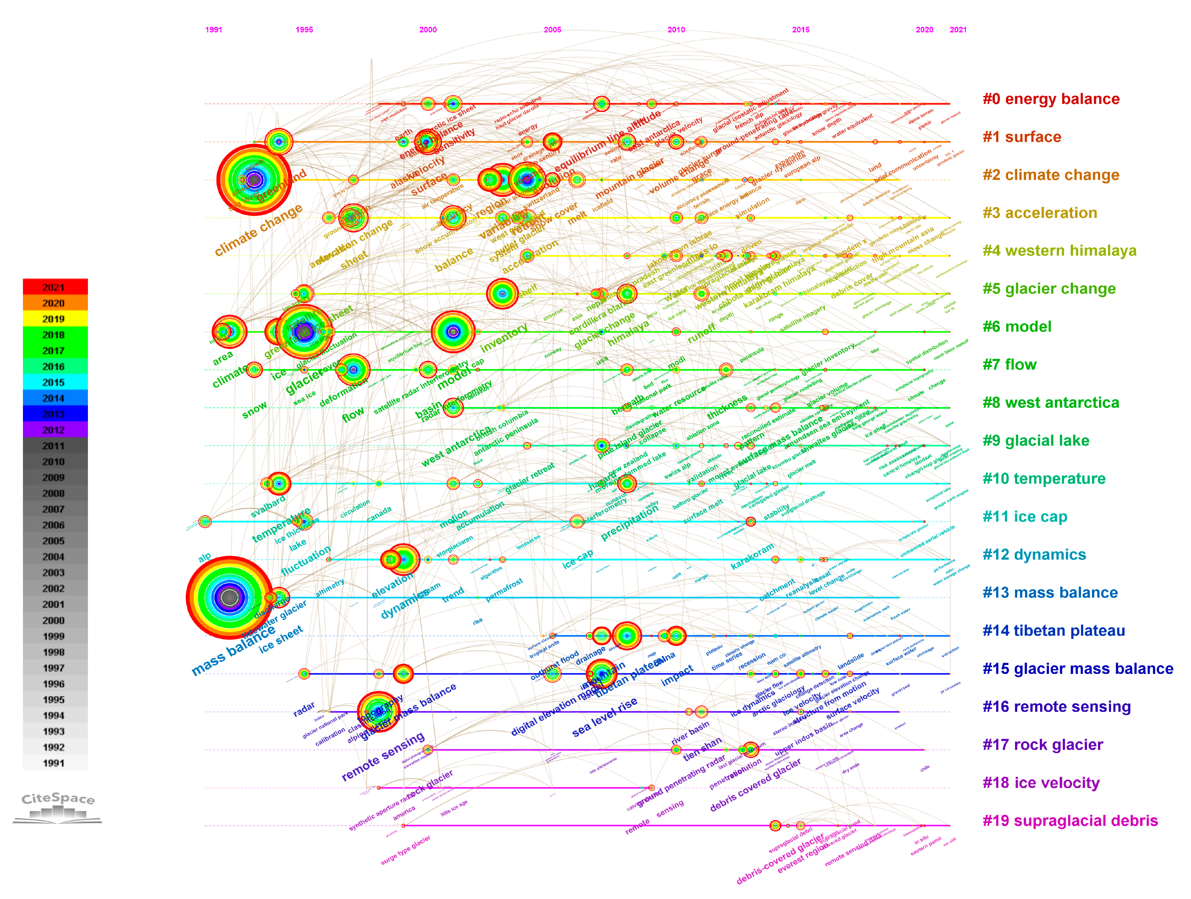
No.	Words	Frequency	Betweenness Centrality
1	Mass balance	962	0.19
2	Climate change	878	0.38
3	Glacier	494	0.34
4	Remote sensing	384	0.10
5	Model	330	0.15
6	Retreat	291	0.12
7	Variability	281	0.22
8	Dynamics	270	0.07
9	Flow	267	0.18
10	Inventory	257	0.35

lists the most frequently occurring keywords, with “Mass balance” appearing most frequently, with 962 occurrences. “Climate change”, “Glacier”, “Remote sensing”, “Model”, “Retreat”, and other relatively large nodes indicate that they are the keywords frequently used by scholars when publishing papers. This is related to the fact that glacier mass balance and remote sensing were used as keywords in the search and that climate change is causing most glaciers to show a retreating trend.

In Table 8, we can see that the keywords with high centrality are “Climate change”, “Inventory”, “Glacier”, and so on. To a certain extent, the research hotspots in the field have been highlighted again. Glaciers are a product of climate change and their changes are a sensitive indicator of climate change.

According to Figure 11, the keyword with the highest burst intensity is “mass balance”, which started in 2001 with an intensity value of 19.63. Glacier mass balance can directly reflect the accumulation and ablation of glacier mass and describes the relationship between climate change and glacier feedback by quantifying the mass changes in glaciers [82,83,84]. Glaciers in most parts of the world are almost in negative balance as a result of global warming, and understanding the dynamics of glacier mass balance and finding its patterns is essential for sea level changes, the security of freshwater resources, and abnormal climate fluctuations research.

By far, the keywords “sea level” and “glacier” have the longest duration of outbreak intensity, lasting 20 and 17 years, respectively. The outbreak of “sea level” started in 1993 and became weaker in 2013. As global temperatures rise, one of the most obvious and important factors affecting sea level rise is the severe retreat of polar and mountain glaciers. The vast majority of glaciers are beginning to melt causing large amounts of water to flow inside the oceans, causing sea level rise. In addition, the latest explosive keyword is “TanDEM-X”, which first appeared in 2018. With the development of science and technology, a TanDEM-X bi-static interferometric image pair released by the German Space Agency not only has high resolution and large coverage, but also has a zero-time baseline, which is not affected by time de-correlation, atmospheric changes, and ground target deformation [85]. TanDEM-X absolute elevation accuracy can reach 10 m, the relative elevation accuracy is 2 m, and the horizontal resolution is 12 m (better than the 30 m resolution of Aster GDEM, which is a US–Japanese collaboration), and the 90 m DEM is currently available for free download. Other keywords such as “Karakoram”, “surface velocity”, and “volume change” are also frequently appearing in 2019. Karakorum is one of the most concentrated regions of surge-type glaciers in the world [86], as Karakorum glaciers exhibit different and irregular glacier movements. For apparently similar or adjacent ice masses, there is little synchronization in their expansion or retreat. In recent years, Karakoram has not experienced the large ice decreases or widespread glacier retreat observed elsewhere in the Himalayas [87]. However, surge glaciers are one of the major causes of ice dams and glacial lake outburst floods, posing a great danger to populated areas and downstream infrastructure and, therefore, systematic studies of Karakorum glaciers are urgently needed. Glacier volume, as an important element of glacier research, is getting more and more attention from researchers. Many scholars have used different methods and tools to study glacier volume changes and have achieved fruitful results, which have important implications for sea level rise, global changes, and regional water cycle studies [88,89,90].

Research frontiers are defined as emerging and transient combinations of concepts and fundamental research that play an important role in promoting practical development applications in the field. Figure 12 shows a timeline of 20 different keyword clusters and their interrelationships. All timelines are arranged from left to right, showing when research keywords appear and disappear. In the timeline diagram, the color bar of the knowledge flow between clusters follows a distribution from dark to light, representing the different stages of development of remote sensing-based studies of glacier mass balance [91]. As shown in

Table 9. High-frequency keywords from 2017 to 2021.

Year	Keywords
2021	water storage change, NDVI, InSAR, land terminating glacier, Google Earth Engine, glacier modeling, extraction, dammed lake, artificial satellite, Artificial intelligence, energy balance model, snow line altitude, hydrological response, machine learning, ICESat-2, KH-9, photogrammetry
2020	glacier dynamics, accuracy assessment, Tibetan plateau, spatial distribution, Pamir, mass change, geodetic method, climate change, Changri Nup Glacier, alpine terrain, area change, glacier flow
2019	glacier volume, ice thickness, glacier surge, classification, satellite gravimetry, risk assessment, lake outburst flood, High Mountain Asia, geodetic mass balance, fresh, Glacial Isostatic Adjustment, elevation model, glacier mapping, glacier hazard, Inventory, time series,
2018	surface velocity, submarine melt, Qilian Mountain, Pine Island, Pamir Karakorum Himalaya, meltwater, grounding line retreat, glacier shrinkage, Central Himalaya, airborne radar, albedo, firn, debris cover
2017	Tandem-x, Karakoram, GRACE, glacier elevation change, DEM generation, upper indus basin, expansion, reconstruction, scale, fusion, remote sensing data

, keywords in 2021 include water storage change, NDVI, Artificial Intelligence, Google Earth Engine, machine learning, photogrammetry, etc. The keywords in 2020 include mass change, glacier dynamics, geodetic method, accuracy assessment, area change, and climate change. The keywords in 2019 include High Mountain Asia, glacier volume, ice thickness, glacier surge, classification, satellite gravimetry, risk assessment, and lake outburst flood. The keywords in 2018 include grounding line retreat, glacier shrinkage, albedo, firn, and debris cover. The keywords in 2017 include Tandem-x, Karakoram, GRACE, glacier elevation change, DEM generation, reconstruction, and fusion.

4. Discussion

In the past few decades, global warming has caused increased melting of glaciers and is a major contributor to the rise in the global mean sea level and an indicator of climate change worldwide. Therefore, the mass changes of polar ice sheets and mountain glaciers have drawn increasing attention from the scientific community and society. Remote sensing technology provides a favorable means for studying the mass balance of glaciers. According to the above experimental analysis, we found that the main methods to estimate the mass balance of glaciers using remote sensing technology include satellite gravimetry, satellite altimetry, the difference of DEM, and the IOM [12,18,92,93,94,95].

4.1. Satellite Gravimetry Method

Satellite gravimetry refers to the direct measurement of glacier mass changes by gravity satellites that can monitor the changes in a time-varying gravity field. Since 2000, the gravity satellite CHAMP, GRACE, and GOCE missions have been gradually launched. Among them, the GRACE satellite uses a K-band ranging system to accurately track the change of distance between the two satellites, which can estimate the change of high-precision time-varying gravity field and earth surface quality. Large-scale glacier mass balance results have now been obtained using this method [12,96,97,98].

At first, this method is widely used in the ice sheet. Velicogna I used the GRACE monthly gravity field model from April 2002 to August 2005 and the optimizing averaging kernel method to estimate the mass change of the Antarctic ice sheet. The results showed that the Antarctic ice sheet had an obvious melting trend at a rate of −152 ± 80 km³/a [99]. Then, GRACE is also increasingly being used in glacier research. Chen JL et al. used GRACE monthly gravity data from April 2002 to November 2005 to study potential long-term mountain glacier melting in southern Alaska and western Canada [100]. The results showed that glacier melting in the Gulf of Alaska (GoA) mountain region is −101 ± 22 km³/yr. Luthcke SB et al. estimated the mass changes of the GoA glaciers from the GRACE inter-satellite range–rate data from April 2003 to March 2007, and they found that the glacier mass balance of the GoA region was –84 ± 5 Gt a^–1 [101]. Matsuo K and Heki K used GRACE from 2003 to 2009 to research the melting of glaciers in the Himalayas, Karakoram Mountains, and Tianshan Mountains, and concluded that the melting rate was −47 ± 12 Gt/yr [14]. Moiwo JP et al. fused GRACE with the climate model and believed that the amount of glacier loss in the Himalayas and Qinghai–Tibet Plateau from January 2003 to December 2008 was 21 ± 1.95 Gt/yr [102]. Compared with GRACE, a GRACE follow-on (GRACE-FO) gravity satellite is equipped with a microwave ranging system as well as laser ranging interferometry (LRI), so it has higher observation accuracy [103]. Ciracì E et al. used GRACE and GRACE-FO to calculate the mass balance of the world’s glaciers and ice caps excluding Antarctica and Greenland peripheral glaciers, of 281.5 ± 30 Gt/yr during 2002–2019 [16].

Satellite gravimetry is the only technique that directly observes mass balance from space. Gravity satellite GRACE can obtain large-scale and large-range glacier mass balance results. It can measure the gravity field of the earth in detail with high time resolution (one month), which can not only provide information about long-term trends but also measure seasonal mass fluctuations [104]. However, there are some sources of uncertainty in applying GRACE to glacier mass balance. The prevailing factor is the uncertainty of glacial isostatic adjustment (GIA) models which is the persistent response of the solid earth due to the changing ice ocean load during the last ice age [105]. GRACE/GRACE-FO itself cannot distinguish the influence of the GIA signal and ice water mass change on the geoid. When applying GRACE/GRACE-FO to estimate the glacier mass balance, the model must be used to deduct the influence of GIA from the geoid change obtained from GRACE/GRACE-FO. At present, the internationally authoritative post-ice rebound models include ICE-4G, ICE-5G, IJ05, RF3L20, etc. [106,107,108]. Due to the use of different load models in different GIA models and the lack of objective understanding of the viscous structure of the mantle, the differences between different post-glacial rebound models are very obvious. In addition, a potential way to mitigate leakage errors which are inherently present due to the rather coarse spatial resolution (a few hundreds of kilometers) of GRACE/GRACE-FO could also be a combination with satellite altimetry and global navigation satellite system (GNSS) data, which offer a much higher spatial resolution.

4.2. Geometric Method

4.2.1. Measurement of Surface Elevation Change

Satellites detecting height changes include GNSS, satellite altimetry [20,109,110], and satellite stereo imagery [19,24].

• Global Navigation Satellite System

The GNSS method uses RTK to systematically and regularly observe the observation points on the glacier and estimate the mass balance of the glacier through the elevation changes of each measurement point. Although the results are accurate, this method is usually limited to a limited number of accessible glaciers, which is difficult to carry out on a large scale and for a long time in areas with complex terrain and harsh environments.

2.

Satellite altimetry

Satellite altimetry includes satellite radar altimetry (SRA) and satellite laser altimetry (SLA). SRA refers to the technology of using the microwave radar altimeter carried by artificial earth satellites to locate the ground point and determine the shape, size, and gravity field of the earth. Early missions such as ERS-1 and 2, Envisat, and SARAL satellites carried traditional low-resolution or pulse-limited instruments. Duncan J first used the ERS1/2 altimetry results to obtain the average annual change rate of the elevation of the Antarctic inland ice sheet from 1992 to 1996, which was 0.9 ± 0.5 cm/yr [111]. In 2013, Lee H et al. estimated the elevation change rate of the Bering Glacier System in Alaska from 1992 to 2010 based on the measurements of Topex/Poseidon(T/P) and Envisat radar altimeters, which proved the feasibility of using SRA on mountain glaciers for the first time [112]. Satellite missions such as ERS1/2, T/P, and Envisat provide important data sources for the status of the cryosphere and its contribution to global sea level rise. However, the radar beam footprint transmitted by the traditional radar altimeter is large, and the measured value is the average value of the surface within the beam range and is only valid for the measured surface with a slope of less than 1°. In addition, the radar signal will penetrate the snow surface, and the return time of the radar pulse will produce errors due to the sharp changes in the elevation of the ice surface, thus affecting the measured elevation value [113].

SAR technology used by CryoSat-2 has increased the resolution along the track to about 400 meters. It also uses interferometric techniques to locate the origin of surface reflection in the cross-track plane, which enhances the performance of altimeters in steep and complex ice margin terrain regions [114]. At the same time, the 92° near-polar orbit can fill the gap of high latitude data of the previous altimetry satellite to some extent and can meet the needs of a high precision, continuous space–time scale in glacier research. McMillan M et al. used Cryosat-2 to develop the first comprehensive assessment of the Antarctic ice sheet’s elevation change. The results show that from 2010 to 2013, the mass of southwest Antarctica, southeast Antarctica, and the Antarctic Peninsula changed by −134 ± 27, −3 ± 36, and −23 ± 8 Gt yr^–1 [115]. Morris A et al. found that the glacier mass change of Svalbard was −16.00 ± 3.00 Gt yr⁻¹ between 2011 and 2017 from Cryosat-2 [116].

The altimeters used in the past are operated in the closed-loop tracking mode, which cannot measure the correct tracking distance in the case of abrupt changes in terrain. In contrast, Sentinel-3 uses an open-loop tracking system operating in delayed Doppler mode throughout the whole glacier area, providing a tracking resolution of 300 meters [117]. It can provide potential benefits for a series of glaciological applications, but at present, it is only used for researching the change of ice sheet elevation.

However, the spatial resolution and data volume of surface water detection using an altimeter based on the track of the nadir are insufficient. For surface water monitoring with a high spatial and temporal resolution, it is expected to be solved by the wide swath microwave altimetry technology. The newly launched surface water and ocean topography (SWOT) altimetry satellite makes the altimetry satellite transition from traditional one-dimensional and orbital profile altimetry to two-dimensional wide swath interference altimetry [118]. Compared with the traditional altimetry satellite pulse limited measurement method, SWOT improves spatial resolution through synthetic aperture radar interferometry. It will have a broad application prospect in monitoring ocean changes and land hydrological changes through the acquisition of high-precision and high-resolution sea surface heights (SSHs) and terrestrial water heights (TWHs) [119].

Compared with radar altimetry, the penetration of high-frequency laser pulses from laser altimetry satellites, such as ICESat, on the glacier surface can be almost negligible, and the problem of radar penetration can be avoided when detecting and estimating the mass balance of the glacier [120]. ICESat has made research achievements in the estimation of glacier mass balance of the Antarctic ice sheet, Greenland, and HMA glaciers [117,121,122,123,124,125]. Neckel N et al. used ICESat for the first time to estimate the elevation and mass changes of glaciers on the Tibetan Plateau between 2003 and 2009. For the Qilian Mountains and eastern Kunlun Mountains, the most negative mass budgets of −0.77 ± 0.35 m w.e. a⁻¹ was discovered, while a mass gain of +0.37 ± 0.25 m w.e. a⁻¹ was discovered in the westerly dominated north central region of the Tibetan Plateau [20]. Based on ICESat satellite altimetry data for the years 2003 to 2008, Kääb A et al. presented glacier thickness changes over the entire Pamir–Karakoram–Himalaya arc, and they discovered that the most negative rate of region-wide glacier elevation change (<−1 m/yr⁻¹) is observed for the eastern Nyainqêntanglha Mountains [66].

The ICESat-2/ATLAS adopted a micro-pulse multi-beam photon-counting laser altimeter system for the first time, which make it is significantly different from CESat-1/GLAS in terms of the detection mechanisms, data processing methods, and the breadth and depth of data applications [111]. ICESat from the spring of 2003 to 2008 and ICESat-2 from the spring of 2019 were utilized by Sochor L et al. to estimate annual elevation and mass change trends over Svalbard. The annual elevation change rate for this period was found to be −0.30 ± 0.15 m yr⁻¹, which corresponds to a mass loss rate of −12.40 ± 4.28 Gt yr⁻¹ [126]. Wang JH et al. calculated the elevation of the Svalbard Islands as −0.775 ± 0.225 m yr⁻¹ and the mass change as −14.843 ± 4.024 Gt yr⁻¹ based on ICESat-2 from 2019 to 2021 [127]. Fan YB et al. compared the elevations from ICESat-2 and the NASADEM to estimate the glacier mass balance over HMA during 2000–2021 and found a remarkable mass loss at Hengduan Shan (−0.62 ± 0.10 m w.e.a⁻¹) [125]. Due to the advantages of the high energy and linearity of laser satellites, points can be measured to an accuracy of decimeters. However, laser altimetry has sparse repeat sampling and a short time span.

3.

DEM differencing

Compared with ICESat, stereo imagery-based studies have the advantages of wider spatial coverage and longer time span. We can obtain DEM based on stereo images. After that, two precise DEMs on different dates are applied to compute the volume change over this time span by means of DEM differencing. A multi-temporal of stereo images is one of the most potential ways to persistently detect glacier state. The study conducted by Bodin X et al. in the French Alps shows that the mass balance value obtained by geodesy had a good correlation with the ground data and had a good correlation with the mass balance reconstruction of meteorological data [128]. Hagg, WJ et al. compared the mass balance estimates of Tuyuksu Glacier using geodetic, glaciological, and hydrological methods. They found good consistency between the geodetic method and field glaciological survey and attributed small differences to errors in the field survey [129].

Reynolds et al. for the first time calculated the changes in the area, elevation, and volume of the Athabasca Glacier in Alberta, Canada by using DEM generated by aerial photogrammetry, and found that the glacier lost 2.344 × 10⁸ m³ of volume and downwasted significantly from 1919 to 1979 [130]. With the development of geodesy and satellite remote sensing technology, DEM data with high accuracy and high spatial and temporal resolution continue to be produced, and geodetic methods are increasingly used to calculate the glacier mass balance. Gardelle J et al. obtained the mass balance results of glaciers in Pamirs–Karakoram–Himalaya from 2000 to 2011 using SPOT-5 stereo pair and SRTM DEM. They found that the region-wide glacier mass balances were contrasted with moderate mass losses in the eastern and central Himalayas [24]. Burn F et al. calculated the mass balance for about 92% of the glacierized area of HMA utilizing time series of DEMs derived from stereo imagery of the Aster satellite. They calculated a total mass change of −16.3 ± 3.5 Gt yr⁻¹ between 2000 and 2016, which is less negative than the majority of the previous estimates [19]. Shean DE et al. estimated that the glacier mass in the HMA region has changed by approximately −19 ± 3 Gt yr⁻¹ from 2000–2018 [131]. However, the accuracy of those products may be inferior to that of laser altimetry. Additionally, they rarely provide information on seasonal variability until now.

There are two main methods to generate DEM. The first is to generate DEM from optical images through photogrammetry technology. Optical remote sensing photogrammetry can extract DEM from stereo image pairs based on the principle of local frontal intersection. Optical stereo image pairs have the characteristics of non-penetrating visible light on ice and snow, and optical remote sensing satellites have the advantages of mature development, high resolution, and a large number of satellites, which is an important technical means to study the mass balance of glaciers [132,133,134,135]. However, most glaciers are high in altitude, with more cloudy and rainy weather and relatively few time windows available for optical remote sensing data selection. In addition, optical remote sensing is prone to light saturation on the glaciers, especially on the snow surface in the accumulation area. Therefore, although the optical stereo pair has the advantages of non-penetration and high resolution on the glacier surface, there are still some limitations in the estimation of glacier mass balance. The other method is synthetic aperture radar (SAR) interferometry. Because microwave signals transmitted by SAR satellites can penetrate clouds and fog, and cover a wide area with high resolution, it has obvious advantages in observing large area and long-term elevation changes. However, most of the SAR satellites use the heavy orbit single transmitter single receiver jamming mode, which is unable to obtain high-precision DEM due to the influence of atmospheric delay, changes in surface scattering characteristics, geometric distortion, and surface deformation. At present, only TanDEM-X images are available for civil satellite synchronous dual orbit single transmitter dual receiver InSAR data sources, resulting in inflexible observation time [136].

Due to the geographical reference error, the original DEM data often appear dislocation, and co-registration is required before the DEM difference. The registration methods can be roughly divided into two categories. One is the data matching method that can be used for DEM rough registration without geographical reference information. For example, the method based on feature points [137], the method based on feature lines [138], the surface matching method based on multiple features [139], the iterative closest point (ICP) algorithm and its variants [140,141], and the least squares 3D surface matching (LS3D) algorithm [142]. However, this method takes a long time to process and is difficult to expand on a large scale. The accuracy of matching depends on a large number of high-quality features. For DEM without sufficient texture, matching will fail. The second category is DEM co-registration methods. This method corresponds each pixel in the slave DEM to the same plane position in the master DEM, minimizing the sum of the vertical distances between the two DEMs. The typical algorithms in this category include grid search methods [143] and terrain information-based methods [144,145]. The method proposed by Nuth C and Kääb A employs the terrain slope and aspect as explanatory variables in the regression model and is currently the most commonly used DEM co-registration algorithm in glacial studies [142].

At present, numerous studies associated with glacier elevation change have been published. However, each of the methods has its own unique characteristics. Altimetry data often have high accuracy, but the spatial coverage is relatively poor. As a result, one limitation of this method is the need to interpolate and extrapolate the original results to obtain dh/dt estimates of the entire glacier volume [95]. DEM derived from photogrammetry or the InSAR method can overcome this limitation in principle, but currently, it cannot provide the accuracy level of laser altimetry or GNSS [146]. Therefore, the methods mentioned above are complementary. The former can provide high-precision results, while the latter has a broader space coverage.

This complementarity has been used in DEM combinations derived from photogrammetry or the InSAR method and satellite altimetry or GNSS to generate dh/dt time series of the limited part of glaciers. Krieger L et al. used CryoSat-2 and TanDEM-X DEM difference for the first time to estimate the mass balance of the two main outlet glaciers of the Northeast Greenland Ice Stream. Between January 2011 and January 2014, the glaciers lost 3.59 ± 1.15 Gt a⁻¹ and 1.01 ± 0.95 Gt a⁻¹, respectively [147]. Zhao F et al. combined satellite altimetry data (ICESat, CryoSat-2, and ICESat-2), DEM difference, and satellite gravity to obtain the time series of elevation change and mass balance of glaciers in the Southeastern Tibetan Plateau (SETP) from 2000 to 2020. Results show rapid and remarkable glacier depletion with a mean mass loss rate of −0.66 ± 0.02 m w.e. yr⁻¹ [148]. Therefore, although the uncertainty of any particular method is sometimes large, the combination of various methods has greatly improved the uncertainty of the glacier mass balance estimation.

4.2.2. Measurement of Area Change

Accurate extraction of glacier area is the basic requirement for glacier mass balance research. At present, the change in the glacier area is generally determined by extracting the glacier boundary in different periods from multi-band remote sensing images [149]. The main methods for extracting bare glacier boundaries include manual visual interpretation and band ratio thresholding, supervised and unsupervised classification, the normalized difference snow index (NDSI), the object-based image analysis method based on multi-scale segmentation, the glacier recognition method based on neural network, and other computer automatic classification methods [150,151,152,153].

Visual interpretation is to artificially divide the boundary between glacial and non-glacial areas by means of multi-band color synthesis of remote sensing images, highlighting the differences between glacial and non-glacial areas in color, texture, hue, and other elements [150]. The advantages of visual interpretation are that it can effectively eliminate the interference of clouds, seasonal snow cover, lake water surface, mountain shadow, and other factors. The smooth boundary of the glacier is closer to the actual situation of the glacier and it can effectively identify the moraine cover area of the glacier, but the disadvantages are low efficiency, the fact that it is easily disturbed by human factors, and diverse identification standards [154].

Unsupervised classification refers to the automatic classification of ground objects according to the statistical distribution law of spectral similarity between pixels without prior category samples [155]. Supervised classification is to extract different kinds of training samples on the training ground of known categories, classify each pixel point in the image into each given category by selecting characteristic variables, and determine discriminant functions or discriminant rules [156]. The ratio threshold method takes advantage of the low reflectivity of ice and snow in the near-infrared (NIR) and short-wave infrared (SWIR) bands and the high reflectivity in the visible light band, and can identify ice and snow by using the reflection characteristics that are different from other ground objects [157]. NDSI uses the difference that ice and snow have on strong reflectivity in a visible light band and absorbs short-wave infrared radiation to distinguish ice and snow from surrounding ground objects [158]. The OBIA is based on a multi-scale segmentation algorithm and spectral characteristics of remote sensing images. When the comprehensive weighted value of all objects to be segmented is greater than a certain threshold, the segmentation is completed. If it is less than the threshold value, the iterative operation will be repeated until the condition is established [159]. The glacier recognition method based on neural networks will learn a large number of samples, extract the characteristic values in the samples, form a classification model, and then classify the remote sensing image [160].

The computer automatic recognition method also has many applications in glacier mapping. Sidjak RW et al. used the supervised classification method, the ratio of 4 and 5 bands of TM images, and NDSI to extract the glacier information from Glacier National Park in Canada [161]. Kaushik et al. proposed an automated scheme for glacier debris mapping using the collaborative method of deep learning and multi-source remote sensing data. Training was conducted at eight locations in the Himalayas and testing was conducted at three locations in the Karakoram region. The results show that the accuracy of the model is 96.3% compared with the experimental data [162]. The advantage of the computer automatic classification method is that it can extract a large range of glacier boundaries in a relatively short time. The disadvantage is that it is easily affected by factors such as clouds, seasonal snow, lake water surface, etc., which makes the glacier boundary not smooth enough, the range area is too large, and the accuracy is poor [162]. How to effectively combine the traditional interpretation method, improve the precision of deep learning glacier information extraction, use effective tags to conduct deep mining and analysis of a large number of data, and reduce the dependence of neural networks on data needs further research.

Generally speaking, many valley glacier ends or tongues are covered by surface moraines. As these surface moraines are mostly from the surrounding bare rock or sandy soil, resulting in similar spectral characteristics between the glacier and the surrounding features, it is difficult to identify the surface moraine-covered areas by optical images alone. Combining the interferometric coherence of SAR image pairs with the glacier surface flow velocity, the localization study of surface moraine-covered glaciers can be effectively carried out. Atwood DK et al. successfully extracted the Taku and Kennicott glaciers and the surrounding areas based on the decoherence characteristics of glaciers on SAR images and systematically discussed the advantages of L-band SAR imagery in the field of glacier identification [163]. At Taku Glacier, Oliver M et al. proposed a method for automatic glacier identification from the perspective of designing a glacier flow model using SAR intensity imagery and using intensity tracking means [164]. In addition, topographic correction and thermal infrared remote sensing are two other methods for surface moraine glacier boundary extraction with high accuracy [165,166].

4.2.3. Volume Conversion Mass

The geometric method is not a direct observation of the mass balance but depends on the assumption that the change of elevation with time (dh/dt) can be converted into the change of mass. This is only true if the rock elevation has not changed as a result of tectonic activity or late ice rebound, and if the density of the ice has not changed. The conversion from elevation change to mass depends on the density model of snow cover [77]. Currently, there are three commonly used models. (1) The interannual change of climate is slow, the glacier dynamics are strong, and the average density of the increased and lost mass of the whole glacier is 900 km/m³. (2) There is no dynamic effect, the climate changes strongly between years, and there are obvious changes in the glacier surface topography. The accumulation area is 600 km/m³ and the melting area is 900 km/m³. (3) The glacier’s elevation change measured by multi-temporal DEM is converted into the glacier’s mass balance, and the interval between the two periods of DEM acquisition is more than 5 years. The average density of the increased and lost mass of the whole glacier is 850 km/m³. In fact, the density varies from one ice layer to another, and there are many errors involved [167].

4.3. Input–Output Method

The IOM differentiates the total input of ice from the total output of ice, in order to derive the change of glacier mass over a time interval, dt [168]. It takes into account two major mass change entities: surface mass balance (SMB) and solid ice discharge (D). The SMB of a glacier is determined by the processes of adding mass to the surface (e.g., snowfall, freezing rain) and by the process of removing mass from the surface (e.g., snow and ice melt, sublimation). D includes both calving and submarine melting at marine-terminating glaciers. SMB is commonly estimated using climate models [169,170,171], whereas D can be estimated by combining measurements of ice thickness and ice velocity [71,172,173].

At present, a large number of studies related to the estimation of glacier mass change by the IOM have been published. Hubbard A et al. first proposed an indirect method for determining mass balance distributions at a high spatial resolution based on the mass continuity equation using remote sensing and ice flow models [174]. Callens D et al. used the IOM to calculate the mass budget of major outlet glaciers in the eastern Dronning Maud Land sector of the Antarctic ice sheet, and they estimated the regional mass balance in this region to be 3.15 ± 8.23 Gt a⁻¹ [175]. Chuter SJ et al. presented a reassessment of ice mass budget estimates for the Abbot and Getz regions of West Antarctica using CryoSat-2-derived ice thickness estimates and the IOM. They found that the mass budget is 8 ± 6 Gt yr⁻¹ and 5 ± 17 Gt yr⁻¹ for the Abbot and Getz sectors, respectively, from 2006 to 2008 [23]. Rignot E et al. calculated the grounding line ice discharge of 176 basins draining the Antarctic ice sheet by using updated drainage inventory, ice thickness, and ice velocity data from 1979 to 2017. Compared with the SMB model, it is inferred that the total mass loss increased during this period [176]. Mouginot J et al. reconstructed the mass balance of the Greenland Ice Sheet using a comprehensive survey of thickness, surface elevation, velocity, and surface mass balance (SMB) of 260 glaciers from 1972 to 2018 [177].

The IOM is the only one that provides information about the physical processes controlling the mass loss, i.e., the partitioning between SMB processes (accumulation minus runoff and other forms of ablation) and glacier dynamics (ice mass flux into the ocean), which is important to inform numerical models [178]. This method’s disadvantage is that it needs to comprehensively and accurately calculate the ice mass flux of glaciers flowing into the ocean and reconstruct the SMB on the ice sheet, and then differentiate the large numbers. Furthermore, only a small number of glaciers have detailed SMB measurements performed because doing so is time-consuming and expensive [179].

In summary, we can estimate the glacier mass balance through three remote sensing methods. However, the glacier mass change results obtained by these three methods under ideal conditions should be highly consistent. In fact, due to different data processing methods or different time periods, the results are definitely inconsistent. For example, three methods have different emphases. The gravity method focuses on the whole and needs to use the model to deduct GIA when estimating the change of glacier mass, but different models have different results. Satellite altimetry focuses on local, single-point sampling and low spatial resolution. The DEM difference method has low elevation accuracy and the IOM is time-consuming and costly, and can only be carried out on a limited number of glaciers. How to improve the consistency of glacier mass changes calculated based on multiple observation methods is a challenge for future research. At present, a large number of satellites have been launched, but it is necessary to further analyze the historical satellite data to solve the problem of data scarcity in the early years. Due to the limited life cycle of each satellite, we can use multiple satellites to obtain a long-term ice mass balance result. However, owing to the differences in spectral and temporal resolution, observation illuminance angle, and sensor band characteristics, data consistency between different sensors needs to be considered [73]. It involves a range of research topics such as the fusion of heterogeneous data from multiple sources, scale conversions, bias calculation methods, etc.

5. Conclusions

With the rapid development of remote sensing technology, glacier mass balance studies based on remote sensing technology have produced a wealth of research. In this study, a bibliometric and visual analysis of remote sensing monitoring studies of glacier mass balance published in English journals from 1990 to 2021 was conducted. This paper summarizes the current research status, research gaps, future research trends, and directions in the use of remote sensing for glacier mass change studies.

In the past three decades, with the revolutionary progress of satellite remote sensing technology, the remote sensing data obtained developed high spatial resolution and high temporal resolution, greatly accelerating the research progress of glacier mass balance. The research can be divided into three main stages in terms of time dimension: the stable starting period (1990–1996), the rapid development period (1997–2006), and the stable development period (2007 to date). The Journal of Glaciology, Geophysical Research Letters, Science, and Annals of Glaciology are the most frequently cited journals by researchers. The analysis of research strength shows that the United States, China, the United Kingdom, Germany, and Switzerland are the countries with the most research achievements. The Chinese Academy of Sciences, the University of Colorado, the University of Zurich, and the CAS California Institute of Technology are the most fruitful research institutions. In terms of output and influence, Rignot E, Kääb A, Bolch T, Paul F, Berthier E, and Huss M are the most outstanding authors.

Hot topics of research in this field are focused on “Climate change”, “Inventory”, “Dynamics”, “Model”, “Retreat”, “Glacier mass balance”, “Sea level”, “Radar”, “Volume change”, “Surface velocity”, “Glacier mapping”, “Hazard”, and other keywords. The current research frontiers mainly include keywords such as water storage change, Artificial Intelligence, High Mountain Asia, photogrammetry, debris cover, geodetic method, area change, glacier volume, classification, satellite gravimetry, grounding line retreat, geodetic mass balance, risk assessment, lake outburst flood, glacier elevation change, DEM generation, etc.

According to the results of the literature visualization analysis, we found that the three commonly used glacier mass balance methods based on remote sensing observation mainly include the satellite gravimetry method, the geometric method, and the IOM, which have been widely and successfully applied in polar ice sheets, mountain glaciers, and other fields. Although these three different technologies are related to each other, they are significantly different in terms of observation objects, accuracy levels, and their own limitations. For example, the spatial resolution of the gravity method is low, the conversion of the geometric method from altitude change to mass is affected by the density model of snow cover, and the input and output method is only applicable to small-area research. These factors affect the research accuracy to a certain extent, leading to the inconsistency of the results obtained by the different methods. With the increasing number and resolution of remote sensing satellites, how to combine multiple methods to achieve high precision long-term glacier quality change monitoring and improve the consistency of results will become the future research trend.

References

- Qin, D.; Zhou, B.; Xiao, C. Progress in studies of cryospheric changes and their impacts on climate of China. J. Meteorol. Res. 2014, 28, 732–746. [Google Scholar] [CrossRef]
- Sorg, A.; Bolch, T.; Stoffel, M.; Solomina, O.; Beniston, M. Climate change impacts on glaciers and runoff in Tien Shan (Central Asia). Nat. Clim. Chang. 2012, 2, 725–731. [Google Scholar] [CrossRef]
- Kraaijenbrink, P.D.A.; Bierkens, M.F.P.; Lutz, A.F.; Immerzeel, W.W. Impact of a global temperature rise of 1.5 degrees Celsius on Asia's glaciers. Nature 2017, 549, 257–260. [Google Scholar] [CrossRef]
- Kääb, A.; Reynolds, J.M.; Haeberli, W. Glacier and Permafrost Hazards in High Mountains. Adv. Global Chang. Res. 2005, 23, 225–234. [Google Scholar]
- Zemp, M.; Hoelzle, M.; Haeberli, W. Six decades of glacier mass-balance observations: A review of the worldwide monitoring network. Ann. Glaciol. 2009, 50, 101–111. [Google Scholar] [CrossRef] [Green Version]
- Yao, T.; Thompson, L.; Yang, W.; Yu, W.; Gao, Y.; Guo, X.; Yang, X.; Duan, K.; Zhao, H.; Xu, B. Different glacier status with atmospheric circulations in Tibetan Plateau and surroundings. Nat. Clim. Chang. 2012, 2, 663–667. [Google Scholar] [CrossRef]
- Mukherjee, K.; Menounos, B.; Shea, J.; Mortezapour, M.; Ednie, M.; Demuth, M.N. Evaluation of surface mass-balance records using geodetic data and physically-based modelling, Place and Peyto glaciers, western Canada. JGlac 2022, 1–18. [Google Scholar] [CrossRef]
- Krampe, D.; Arndt, A.; Schneider, C. Energy and glacier mass balance of Fürkeleferner, Italy: Past, present, and future. Front. Earth Sci. 2022, 10, 814027. [Google Scholar] [CrossRef]
- Peng, J.; Xu, L.; Li, Z.; Chen, P.; Luo, Y.; Cao, C. Study on Change of the Glacier Mass Balance and Its Response to Extreme Climate of Urumqi Glacier No. 1 in Tianshan Mountains in Recent 41 Years. Water 2022, 14, 2982. [Google Scholar] [CrossRef]
- Guruprasad, C.; Gopal, D.; Devaraj, S. Mass balance estimation of Mulkila glacier, Western Himalayas, using glacier melt model. Environ. Monit. Assess. 2022, 194, 761. [Google Scholar]
- Xiang, L.; Wang, H.; Jiang, L.; Shen, Q.; Steffen, H.; Li, Z. Glacier mass balance in High Mountain Asia inferred from a GRACE release-6 gravity solution for the period 2002–2016. J. Arid. Land 2021, 13, 224–238. [Google Scholar] [CrossRef]
- Wouters, B.; Gardner, A.S.; Moholdt, G. Global glacier mass loss during the GRACE satellite mission (2002–2016). Front. Earth Sci. 2019, 7, 96. [Google Scholar] [CrossRef] [Green Version]
- Yi, S.; Sun, W. Evaluation of glacier changes in high-mountain Asia based on 10 year GRACE RL05 models. J. Geophys. Res. Solid Earth 2014, 119, 2504–2517. [Google Scholar] [CrossRef]
- Matsuo, K.; Heki, K. Time-variable ice loss in Asian high mountains from satellite gravimetry. Earth Planet. Sci. Lett. 2010, 290, 30–36. [Google Scholar] [CrossRef]
- Velicogna, I.; Mohajerani, Y.; Landerer, F.; Mouginot, J.; Noel, B.; Rignot, E.; Sutterley, T.; van den Broeke, M.; van Wessem, M.; Wiese, D. Continuity of ice sheet mass loss in Greenland and Antarctica from the GRACE and GRACE Follow-On missions. Geophys. Res. Lett. 2020, 47, e2020GL087291. [Google Scholar] [CrossRef] [Green Version]
- Ciracì, E.; Velicogna, I.; Swenson, S. Continuity of the mass loss of the world's glaciers and ice caps from the GRACE and GRACE Follow-On missions. Geophys. Res. Lett. 2020, 47, e2019GL086926. [Google Scholar] [CrossRef]
- Hugonnet, R.; McNabb, R.; Berthier, E.; Menounos, B.; Nuth, C.; Girod, L.; Farinotti, D.; Huss, M.; Dussaillant, I.; Brun, F. Accelerated global glacier mass loss in the early twenty-first century. Nature 2021, 592, 726–731. [Google Scholar] [CrossRef]
- Yan, L.; Wang, J.; Shao, D. Glacier Mass Balance in the Manas River Using Ascending and Descending Pass of Sentinel 1A/1B Data and SRTM DEM. Remote Sens. 2022, 14, 1506. [Google Scholar] [CrossRef]
- Brun, F.; Berthier, E.; Wagnon, P.; Kääb, A.; Treichler, D. A spatially resolved estimate of High Mountain Asia glacier mass balances from 2000 to 2016. Nat. Geosci. 2017, 10, 668–673. [Google Scholar] [CrossRef] [Green Version]
- Neckel, N.; Kropáček, J.; Bolch, T.; Hochschild, V. Glacier mass changes on the Tibetan Plateau 2003–2009 derived from ICESat laser altimetry measurements. Environ. Res. Lett. 2014, 9, 014009. [Google Scholar] [CrossRef]
- Smith, B.E.; Sutterley, T.C.; Alexander, P.; Tedesco, M.; Medley, B.; Fettweis, X. Evaluating Greenland Surface Mass Balance and Firn Density Models with ICESat-2 altimetry differences. Cryosphere 2023, 17, 789–808. [Google Scholar] [CrossRef]
- Jakob, L.; Gourmelen, N.; Ewart, M.; Plummer, S. Spatially and temporally resolved ice loss in High Mountain Asia and the Gulf of Alaska observed by CryoSat-2 swath altimetry between 2010 and 2019. Cryosphere 2021, 15, 1845–1862. [Google Scholar] [CrossRef]
- Chuter, S.; Martín-Español, A.; Wouters, B.; Bamber, J.L. Mass balance reassessment of glaciers draining into the Abbot and Getz Ice Shelves of West Antarctica. Geophys. Res. Lett. 2017, 44, 7328–7337. [Google Scholar] [CrossRef]
- Gardelle, J.; Berthier, E.; Arnaud, Y.; Kääb, A. Region-wide glacier mass balances over the Pamir-Karakoram-Himalaya during 1999–2011. Cryosphere 2013, 7, 1263–1286. [Google Scholar] [CrossRef] [Green Version]
- Falaschi, D.; Berthier, E.; Belart, J.M.; Bravo, C.; Castro, M.; Durand, M.; Villalba, R. Increased mass loss of glaciers in Volcán Domuyo (Argentinian Andes) between 1962 and 2020, revealed by aerial photos and satellite stereo imagery. JGlac 2022, 1–17. [Google Scholar] [CrossRef]
- Bollen, K.E.; Enderlin, E.M.; Muhlheim, R. Dynamic mass loss from Greenland's marine-terminating peripheral glaciers (1985–2018). JGlac 2022, 1–11. [Google Scholar] [CrossRef]
- Raman, A.; Kulkarni, A.V.; Prasad, V. Glacier mass balance estimation in Garhwal Himalaya using improved accumulation area ratio method. Environ. Monit. Assess. 2022, 194, 1–16. [Google Scholar] [CrossRef]
- Livingstone, S.J.; Li, Y.; Rutishauser, A.; Sanderson, R.J.; Winter, K.; Mikucki, J.A.; Björnsson, H.; Bowling, J.S.; Chu, W.; Dow, C.F. Subglacial lakes and their changing role in a warming climate. Nat. Rev. Earth Environ. 2022, 3, 106–124. [Google Scholar] [CrossRef]
- Zekollari, H.; Huss, M.; Farinotti, D.; Lhermitte, S. Ice-Dynamical Glacier Evolution Modeling—A Review. RvGeo 2022, 60, e2021RG000754. [Google Scholar] [CrossRef]
- Rashid, H.F. Bibliometric analysis as a tool in journal evaluation. Ser Libr 1991, 20, 55–64. [Google Scholar] [CrossRef]
- Quade, E.S. On the Limitations of Quantitative Analysis; Rand Corp.: Santa Monica, CA, USA, 1970. [Google Scholar]
- Vail, E.F. Knowledge mapping: Getting started with knowledge management. Inf. Syst. Manag. 1999, 16, 1–8. [Google Scholar] [CrossRef]
- Rastogi, R.; Sharma, T. Quantitative analysis of drainage basin characteristics. J. Soil Water Conserv. 2022, 26, 18–25. [Google Scholar]
- Adamopoulos, T.; Brandt, L.; Leight, J.; Restuccia, D. Misallocation, selection, and productivity: A quantitative analysis with panel data from china. Econometrica 2022, 90, 1261–1282. [Google Scholar] [CrossRef]
- Yang, S.; Li, X. Derivation of ambiguity in wavefront aberration and quantitative analysis in ao system. OptLE 2022, 158, 107174. [Google Scholar] [CrossRef]
- Li, K.; Rollins, J.; Yan, E. Web of Science use in published research and review papers 1997–2017: A selective, dynamic, cross-domain, content-based analysis. Scim 2018, 115, 1–20. [Google Scholar] [CrossRef] [Green Version]
- Chen, C. Science mapping: A systematic review of the literature. J. Data Inf. Sci. 2017, 2, 1–40. [Google Scholar] [CrossRef] [Green Version]
- Hood, W.; Wilson, C. The literature of bibliometrics, scientometrics, and informetrics. Scim 2001, 52, 291–314. [Google Scholar]
- Keim, D.A. Information visualization and visual data mining. IEEE Trans. Visual. Comput. Graphics 2002, 8, 1–8. [Google Scholar] [CrossRef]
- Broadus, R.N. Toward a definition of “bibliometrics”. Scim 1987, 12, 373–379. [Google Scholar] [CrossRef]
- Chen, C.; Hu, Z.; Liu, S.; Tseng, H. Emerging trends in regenerative medicine: A scientometric analysis in CiteSpace. Expert. Opin. Biol. Ther. 2012, 12, 593–608. [Google Scholar] [CrossRef]
- Kousha, K.; Levitt, J. Michael Thelwall wins the 2015 Derek John de Solla Price Medal. Scientometr. Int. J. All Quant. Asp. Sci. Sci. Policy 2016, 108, 485–488. [Google Scholar] [CrossRef] [Green Version]
- Heid, T.; Kääb, A. Evaluation of existing image matching methods for deriving glacier surface displacements globally from optical satellite imagery. Rem. Sens. Environ. 2012, 118, 339–355. [Google Scholar] [CrossRef]
- Xie, P. Study of international anticancer research trends via co-word and document co-citation visualization analysis. Scim 2015, 105, 611–622. [Google Scholar] [CrossRef]
- Chen, C. CiteSpace II: Detecting and visualizing emerging trends and transient patterns in scientific literature. JASIS 2006, 57, 359–377. [Google Scholar] [CrossRef] [Green Version]
- Shean, D.E.; Joughin, I.R.; Dutrieux, P.; Smith, B.E.; Berthier, E. Ice shelf basal melt rates from a high-resolution digital elevation model (DEM) record for Pine Island Glacier, Antarctica. Cryosphere 2019, 13, 2633–2656. [Google Scholar] [CrossRef] [Green Version]
- Berthier, E.; Brun, F. Karakoram geodetic glacier mass balances between 2008 and 2016: Persistence of the anomaly and influence of a large rock avalanche on Siachen Glacier. JGlac 2019, 65, 494–507. [Google Scholar] [CrossRef] [Green Version]
- Björnsson, H.; Pálsson, F.; Gudmundsson, S.; Magnússon, E.; Adalgeirsdóttir, G.; Jóhannesson, T.; Berthier, E.; Sigurdsson, O.; Thorsteinsson, T. Contribution of Icelandic ice caps to sea level rise: Trends and variability since the Little Ice Age. Geophys. Res. Lett. 2013, 40, 1546–1550. [Google Scholar] [CrossRef]
- Gardner, A.S.; Moholdt, G.; Cogley, J.G.; Wouters, B.; Arendt, A.A.; Wahr, J.; Berthier, E.; Hock, R.; Pfeffer, W.T.; Kaser, G. A reconciled estimate of glacier contributions to sea level rise: 2003 to 2009. Science 2013, 340, 852–857. [Google Scholar] [CrossRef] [Green Version]
- Toutin, T.; Schmitt, C.; Berthier, E.; Clavet, D. DEM generation over ice fields in the Canadian Arctic with along-track SPOT5 HRS stereo data. CaJRS 2011, 37, 429–438. [Google Scholar] [CrossRef]
- Berthier, E.; Toutin, T. SPOT5-HRS digital elevation models and the monitoring of glacier elevation changes in North-West Canada and South-East Alaska. Rem. Sens. Environ. 2008, 112, 2443–2454. [Google Scholar] [CrossRef]
- Błaszczyk, M.; Ignatiuk, D.; Grabiec, M.; Kolondra, L.; Laska, M.; Decaux, L.; Jania, J.; Berthier, E.; Luks, B.; Barzycka, B. Quality assessment and glaciological applications of digital elevation models derived from space-borne and aerial images over two tidewater glaciers of southern Spitsbergen. Remote Sens. 2019, 11, 1121. [Google Scholar] [CrossRef] [Green Version]
- Das, I.; Hock, R.; Berthier, E.; Lingle, C.S. 21st-century increase in glacier mass loss in the Wrangell Mountains, Alaska, USA, from airborne laser altimetry and satellite stereo imagery. JGlac 2014, 60, 283–293. [Google Scholar] [CrossRef] [Green Version]
- Drolon, V.; Maisongrande, P.; Berthier, E.; Swinnen, E.; Huss, M. Monitoring of seasonal glacier mass balance over the European Alps using low-resolution optical satellite images. JGlac 2016, 62, 912–927. [Google Scholar] [CrossRef] [Green Version]
- Hu, W.; Li, C.-h.; Ye, C.; Wang, J.; Wei, W.-w.; Deng, Y. Research progress on ecological models in the field of water eutrophication: CiteSpace analysis based on data from the ISI web of science database. Ecol. Modell. 2019, 410, 108779. [Google Scholar]
- Small, H. Co-citation in the scientific literature: A new measure of the relationship between two documents. J. Am. Soc. Inf. Sci. 1973, 24, 265–269. [Google Scholar]
- Chen, C. Visualizing and exploring scientific literature with Citespace: An introduction. In Proceedings of the 2018 Conference on Human Information Interaction & Retrieval, New Brunswick, NJ, USA, 11–15 March 2018; pp. 369–370. [Google Scholar]
- Ren, S.; Menenti, M.; Jia, L.; Zhang, J.; Zhang, J. Glacier Mass Balance in the Kangri Karpo Mountains by ZY-3 Stereo Images and SRTM DEMs Between 2000 and 2017. In Proceedings of the IGARSS 2019—2019 IEEE International Geoscience and Remote Sensing Symposium, Yokohama, Japan, 28 July–2 August 2019; pp. 4153–4156. [Google Scholar]
- Liu, S.; Sun, Y.-P.; Gao, X.-L.; Sui, Y. Knowledge domain and emerging trends in Alzheimer’s disease: A scientometric review based on CiteSpace analysis. Neural Regen Res. 2019, 14, 1643. [Google Scholar]
- Pfeffer, W.T.; Arendt, A.A.; Bliss, A.; Bolch, T.; Cogley, J.G.; Gardner, A.S.; Hagen, J.-O.; Hock, R.; Kaser, G.; Kienholz, C. The Randolph Glacier Inventory: A globally complete inventory of glaciers. JGlac 2014, 60, 537–552. [Google Scholar] [CrossRef] [Green Version]
- Bolch, T.; Kulkarni, A.; Kääb, A.; Huggel, C.; Paul, F.; Cogley, J.G.; Frey, H.; Kargel, J.S.; Fujita, K.; Scheel, M. The state and fate of Himalayan glaciers. Science 2012, 336, 310–314. [Google Scholar] [CrossRef] [Green Version]
- Kääb, A.; Berthier, E.; Nuth, C.; Gardelle, J.; Arnaud, Y. Contrasting patterns of early twenty-first-century glacier mass change in the Himalayas. Nature 2012, 488, 495–498. [Google Scholar] [CrossRef]
- Jacob, T.; Wahr, J.; Pfeffer, W.T.; Swenson, S. Recent contributions of glaciers and ice caps to sea level rise. Nature 2012, 482, 514–518. [Google Scholar]
- Shepherd, A.; Ivins, E.R.; Barletta, V.R.; Bentley, M.J.; Bettadpur, S.; Briggs, K.H.; Bromwich, D.H.; Forsberg, R.; Galin, N.; Horwath, M. A reconciled estimate of ice-sheet mass balance. Science 2012, 338, 1183–1189. [Google Scholar] [CrossRef] [Green Version]
- Paul, F.; Barrand, N.E.; Baumann, S.; Berthier, E.; Bolch, T.; Casey, K.; Frey, H.; Joshi, S.; Konovalov, V.; Le Bris, R. On the accuracy of glacier outlines derived from remote-sensing data. Ann. Glaciol. 2013, 54, 171–182. [Google Scholar] [CrossRef] [Green Version]
- Kääb, A.; Treichler, D.; Nuth, C.; Berthier, E. Brief Communication: Contending estimates of 2003–2008 glacier mass balance over the Pamir–Karakoram–Himalaya. Cryosphere 2015, 9, 557–564. [Google Scholar] [CrossRef] [Green Version]
- Huss, M.; Hock, R. Global-scale hydrological response to future glacier mass loss. Nat. Clim. Chang. 2018, 8, 135–140. [Google Scholar] [CrossRef] [Green Version]
- Cuffey, K.M.; Paterson, W. The Physics of Glaciers, 4th ed.; Butterworth-Heinemann: Oxford, UK, 2010. [Google Scholar]
- Meier, M.F.; Dyurgerov, M.B.; Rick, U.K.; O'neel, S.; Pfeffer, W.T.; Anderson, R.S.; Anderson, S.P.; Glazovsky, A.F. Glaciers dominate eustatic sea-level rise in the 21st century. Science 2007, 317, 1064–1067. [Google Scholar] [CrossRef] [Green Version]
- Pritchard, H.D.; Arthern, R.J.; Vaughan, D.G.; Edwards, L.A. Extensive dynamic thinning on the margins of the Greenland and Antarctic ice sheets. Nature 2009, 461, 971–975. [Google Scholar] [CrossRef]
- Rignot, E.; Kanagaratnam, P. Changes in the velocity structure of the Greenland Ice Sheet. Science 2006, 311, 986–990. [Google Scholar] [CrossRef] [Green Version]
- Scherler, D.; Bookhagen, B.; Strecker, M.R. Spatially variable response of Himalayan glaciers to climate change affected by debris cover. Nat. Geosci. 2011, 4, 156–159. [Google Scholar] [CrossRef]
- Nuth, C.; Kääb, A. Co-registration and bias corrections of satellite elevation data sets for quantifying glacier thickness change. Cryosphere 2011, 5, 271–290. [Google Scholar] [CrossRef] [Green Version]
- Rignot, E.; Velicogna, I.; van den Broeke, M.R.; Monaghan, A.; Lenaerts, J.T. Acceleration of the contribution of the Greenland and Antarctic ice sheets to sea level rise. Geophys. Res. Lett 2011, 38, L05503. [Google Scholar] [CrossRef] [Green Version]
- Bolch, T.; Menounos, B.; Wheate, R. Landsat-based inventory of glaciers in western Canada, 1985–2005. Remote Sens. Environ. 2010, 114, 127–137. [Google Scholar] [CrossRef]
- Guo, W.; Liu, S.; Xu, J.; Wu, L.; Shangguan, D.; Yao, X.; Wei, J.; Bao, W.; Yu, P.; Liu, Q. The second Chinese glacier inventory: Data, methods and results. JGlac 2015, 61, 357–372. [Google Scholar]
- Huss, M. Density assumptions for converting geodetic glacier volume change to mass change. Cryosphere 2013, 7, 877–887. [Google Scholar]
- Immerzeel, W.W.; Van Beek, L.P.; Bierkens, M.F. Climate change will affect the Asian water towers. Science 2010, 328, 1382–1385. [Google Scholar] [CrossRef]
- Shean, D.E.; Alexandrov, O.; Moratto, Z.M.; Smith, B.E.; Joughin, I.R.; Porter, C.; Morin, P. An automated, open-source pipeline for mass production of digital elevation models (DEMs) from very-high-resolution commercial stereo satellite imagery. ISPRS J. Photogramm. Remote Sens. 2016, 116, 101–117. [Google Scholar] [CrossRef] [Green Version]
- Zemp, M.; Frey, H.; Gärtner-Roer, I.; Nussbaumer, S.U.; Hoelzle, M.; Paul, F.; Haeberli, W.; Denzinger, F.; Ahlstrøm, A.P.; Anderson, B. Historically unprecedented global glacier decline in the early 21st century. JGlac 2015, 61, 745–762. [Google Scholar] [CrossRef] [Green Version]
- Wang, L.; Zhang, G.; Wang, Z.; Liu, J.; Shang, J.; Liang, L. Bibliometric analysis of remote sensing research trend in crop growth monitoring: A case study in China. Remote Sens. 2019, 11, 809. [Google Scholar] [CrossRef] [Green Version]
- Hao, H.; Hao, Y.; Liu, Y.; Yeh, T.-C.J.; Zhang, M.; Wang, Q.; Fan, Y. Anomaly of glacier mass balance in different vertical zones and responses to climate modes: Urumqi Glacier No. 1, China. ClDy 2022, 1–17. [Google Scholar] [CrossRef]
- O'Neel, S.; McNeil, C.; Sass, L.C.; Florentine, C.; Baker, E.H.; Peitzsch, E.; McGrath, D.; Fountain, A.G.; Fagre, D. Reanalysis of the US Geological Survey Benchmark Glaciers: Long-term insight into climate forcing of glacier mass balance. JGlac 2019, 65, 850–866. [Google Scholar] [CrossRef] [Green Version]
- Liang, L.; Cuo, L.; Liu, Q. Mass balance variation and associative climate drivers for the Dongkemadi Glacier in the central Tibetan Plateau. J. Geophys. Res. 2019, 124, 10814–10825. [Google Scholar] [CrossRef]
- Floricioiu, D.; Jaber, W.A.; Minet, C.; Rossi, C.; Eineder, M. Tandem-X for mass balance of glaciers and subglacial volcanic activities. In Proceedings of the 2015 IEEE International Geoscience and Remote Sensing Symposium (IGARSS), Milan, Italy, 26–31 July 2015; pp. 2903–2906. [Google Scholar]
- Masiokas, M.H.; Rabatel, A.; Rivera, A.; Ruiz, L.; Pitte, P.; Ceballos, J.L.; Barcaza, G.; Soruco, A.; Bown, F.; Berthier, E. A review of the current state and recent changes of the Andean cryosphere. Front. Earth Sci. 2020, 8, 99. [Google Scholar] [CrossRef]
- Zhang, X.; Zhang, S.; Xu, J. Glacier stagnant in central Karakorum during 2003 to 2008 derived from DEOS Mass Transport Model GRACE data and one monthly degree-day model. In Proceedings of the Remote Sensing for Agriculture, Ecosystems, and Hydrology XVIII, Edinburgh, UK, 26–29 September 2016; pp. 48–59. [Google Scholar]
- Huh, K.I.; Mark, B.G.; Ahn, Y.; Hopkinson, C. Volume change of tropical Peruvian glaciers from multi-temporal digital elevation models and volume–surface area scaling. Geogr. Ann. Ser. A Phys. Geogr. 2017, 99, 222–239. [Google Scholar] [CrossRef]
- Pandey, A.C.; Ghosh, S.; Nathawat, M.; Tiwari, R.K. Area change and thickness variation over Pensilungpa Glacier (J&K) using remote sensing. J. Indian Soc. Remote Sens. 2012, 40, 245–255. [Google Scholar]
- Surazakov, A.B.; Aizen, V.B. Estimating volume change of mountain glaciers using SRTM and map-based topographic data. IEEE Trans. Geosci. Remote Sens. 2006, 44, 2991–2995. [Google Scholar] [CrossRef]
- Liu, Z. Current Situation and Development Trend of Ideological and Cultural Psychology Research in the Context of the COVID-19 Epidemic-Knowledge Graph Analysis Based on Citespace. Psychiatr. Danub. 2022, 34, S878–S890. [Google Scholar]
- Mohajerani, Y.; Velicogna, I.; Rignot, E. Mass loss of Totten and Moscow University Glaciers, East Antarctica, using regionally optimized GRACE mascons. Geophys. Res. Lett. 2018, 45, 7010–7018. [Google Scholar] [CrossRef] [Green Version]
- Zhou, Y.; Li, Z.; Li, J.; Zhao, R.; Ding, X. Geodetic glacier mass balance (1975–1999) in the central Pamir using the SRTM DEM and KH-9 imagery. JGlac 2019, 65, 309–320. [Google Scholar] [CrossRef] [Green Version]
- Bolch, T.; Sandberg Sørensen, L.; Simonsen, S.B.; Mölg, N.; Machguth, H.; Rastner, P.; Paul, F. Mass loss of Greenland's glaciers and ice caps 2003–2008 revealed from ICESat laser altimetry data. Geophys. Res. Lett. 2013, 40, 875–881. [Google Scholar] [CrossRef] [Green Version]
- Moholdt, G.; Nuth, C.; Hagen, J.O.; Kohler, J. Recent elevation changes of Svalbard glaciers derived from ICESat laser altimetry. Rem. Sens. Environ. 2010, 114, 2756–2767. [Google Scholar] [CrossRef]
- Jin, S.; Zou, F. Re-estimation of glacier mass loss in Greenland from GRACE with correction of land–ocean leakage effects. GPC 2015, 135, 170–178. [Google Scholar] [CrossRef]
- Zou, F.; Tenzer, R.; Fok, H.S.; Nichol, J.E. Mass balance of the Greenland ice sheet from GRACE and surface mass balance modelling. Water 2020, 12, 1847. [Google Scholar] [CrossRef]
- Richter, A.; Groh, A.; Horwath, M.; Ivins, E.; Marderwald, E.; Hormaechea, J.L.; Perdomo, R.; Dietrich, R. The rapid and steady mass loss of the patagonian icefields throughout the GRACE era: 2002–2017. Remote Sens. 2019, 11, 909. [Google Scholar] [CrossRef] [Green Version]
- Velicogna, I.; Wahr, J. Measurements of time-variable gravity show mass loss in Antarctica. Science 2006, 311, 1754–1756. [Google Scholar] [CrossRef] [PubMed] [Green Version]
- Chen, J.; Tapley, B.; Wilson, C. Alaskan mountain glacial melting observed by satellite gravimetry. Earth Planet. Sci. Lett. 2006, 248, 368–378. [Google Scholar] [CrossRef]
- Luthcke, S.B.; Arendt, A.A.; Rowlands, D.D.; McCarthy, J.J.; Larsen, C.F. Recent glacier mass changes in the Gulf of Alaska region from GRACE mascon solutions. JGlac 2008, 54, 767–777. [Google Scholar] [CrossRef] [Green Version]
- Moiwo, J.P.; Yang, Y.; Tao, F.; Lu, W.; Han, S. Water storage change in the Himalayas from the Gravity Recovery and Climate Experiment (GRACE) and an empirical climate model. WRR 2011, 47. [Google Scholar] [CrossRef] [Green Version]
- Abich, K.; Abramovici, A.; Amparan, B.; Baatzsch, A.; Okihiro, B.B.; Barr, D.C.; Bize, M.P.; Bogan, C.; Braxmaier, C.; Burke, M.J. In-orbit performance of the GRACE follow-on laser ranging interferometer. PhRvL 2019, 123, 031101. [Google Scholar] [CrossRef] [Green Version]
- Chen, J.; Cazenave, A.; Dahle, C.; Llovel, W.; Panet, I.; Pfeffer, J.; Moreira, L. Applications and challenges of GRACE and GRACE follow-on satellite gravimetry. SGeo 2022, 43, 305–345. [Google Scholar] [CrossRef]
- Gao, C.-C.; Lu, Y.; Shi, H.-L.; Zhang, Z.-Z.; Jiang, Y.-T. Combination of GRACE and ICESat data sets to estimate Antarctica Glacial Isostatic Adjustment (GIA). ChJG 2016, 59, 4007–4021. [Google Scholar]
- Wang, H.-s.; Wu, P.; Xu, H.-z. A review of research in glacial isostatic adjustment. Prog. Geophys. 2009, 24, 1958–1967. [Google Scholar]
- Peltier, W.R. Global glacial isostasy and the surface of the ice-age Earth: The ICE-5G (VM2) model and GRACE. Annu. Rev. Earth Planet. Sci. 2004, 32, 111–149. [Google Scholar] [CrossRef]
- Ivins, E.R.; James, T.S. Antarctic glacial isostatic adjustment: A new assessment. Antarct. Sci. 2005, 17, 541–553. [Google Scholar] [CrossRef] [Green Version]
- Wang, Q.; Yi, S.; Chang, L.; Sun, W. Large-scale seasonal changes in glacier thickness across High Mountain Asia. Geophys. Res. Lett. 2017, 44, 10427–10435. [Google Scholar] [CrossRef]
- Treichler, D.; Kääb, A.; Salzmann, N.; Xu, C.-Y. Recent glacier and lake changes in High Mountain Asia and their relation to precipitation changes. Cryosphere 2019, 13, 2977–3005. [Google Scholar] [CrossRef] [Green Version]
- Wingham, D.J.; Ridout, A.J.; Scharroo, R.; Arthern, R.J.; Shum, C. Antarctic elevation change from 1992 to 1996. Science 1998, 282, 456–458. [Google Scholar] [CrossRef] [PubMed]
- Lee, H.; Shum, C.; Tseng, K.-H.; Huang, Z.; Sohn, H.-G. Elevation changes of Bering Glacier System, Alaska, from 1992 to 2010, observed by satellite radar altimetry. Rem. Sens. Environ. 2013, 132, 40–48. [Google Scholar] [CrossRef]
- Brenner, A.C.; DiMarzio, J.P.; Zwally, H.J. Precision and accuracy of satellite radar and laser altimeter data over the continental ice sheets. IEEE Trans. Geosci. Remote Sens. 2007, 45, 321–331. [Google Scholar] [CrossRef]
- Wingham, D.; Francis, C.; Baker, S.; Bouzinac, C.; Brockley, D.; Cullen, R.; de Chateau-Thierry, P.; Laxon, S.; Mallow, U.; Mavrocordatos, C. CryoSat: A mission to determine the fluctuations in Earth’s land and marine ice fields. AdSpR 2006, 37, 841–871. [Google Scholar] [CrossRef]
- McMillan, M.; Shepherd, A.; Sundal, A.; Briggs, K.; Muir, A.; Ridout, A.; Hogg, A.; Wingham, D. Increased ice losses from Antarctica detected by CryoSat-2. Geophys. Res. Lett. 2014, 41, 3899–3905. [Google Scholar] [CrossRef]
- Morris, A.; Moholdt, G.; Gray, L. Spread of Svalbard glacier mass loss to Barents Sea margins revealed by CryoSat-2. J. Geophys. Res. Earth Surf. 2020, 125, e2019JF005357. [Google Scholar] [CrossRef]
- Li, S.; Liao, J.; Zhang, L. Extraction and analysis of elevation changes in Antarctic ice sheet from CryoSat-2 and Sentinel-3 radar altimeters. J. Appl. Remote Sens. 2022, 16, 034514. [Google Scholar]
- Elmer, N.J.; Hain, C.; Hossain, F.; Desroches, D.; Pottier, C. Generating proxy SWOT water surface elevations using WRF-Hydro and the CNES SWOT Hydrology Simulator. WRR 2020, 56, e2020WR027464. [Google Scholar] [CrossRef]
- Biancamaria, S.; Lettenmaier, D.P.; Pavelsky, T.M. The SWOT mission and its capabilities for land hydrology. In Remote Sensing and Water Resources; Springer: Berlin/Heidelberg, Germany, 2016; pp. 117–147. [Google Scholar]
- Rott, H.; Scheiblauer, S.; Wuite, J.; Krieger, L.; Floricioiu, D.; Rizzoli, P.; Libert, L.; Nagler, T. Penetration of interferometric radar signals in Antarctic snow. Cryosphere 2021, 15, 4399–4419. [Google Scholar] [CrossRef]
- Jin, S.; Zhang, T.; Zou, F. Glacial density and GIA in Alaska estimated from ICESat, GPS and GRACE measurements. J. Geophys. Res. Earth Surf. 2017, 122, 76–90. [Google Scholar] [CrossRef]
- Zwally, H.J.; Li, J.; Robbins, J.W.; Saba, J.L.; Yi, D.; Brenner, A.C. Mass gains of the Antarctic ice sheet exceed losses. JGlac 2015, 61, 1019–1036. [Google Scholar] [CrossRef] [Green Version]
- Zou, F.; Jin, S. Estimations of glacier melting in Greenland from combined satellite gravimetry and icesat. In Proceedings of the 2016 IEEE International Geoscience and Remote Sensing Symposium (IGARSS), Beijing, China, 10–15 July 2016; pp. 6185–6188. [Google Scholar]
- Chen, G.; Zhang, S. Elevation and volume change determination of Greenland Ice Sheet based on icesat observations. ChJG 2019, 62, 2417–2428. [Google Scholar]
- Fan, Y.; Ke, C.-Q.; Zhou, X.; Shen, X.; Yu, X.; Lhakpa, D. Glacier mass-balance estimates over High Mountain Asia from 2000 to 2021 based on ICESat-2 and NASADEM. JGlac 2022, 1–13. [Google Scholar] [CrossRef]
- Sochor, L.; Seehaus, T.; Braun, M.H. Increased ice thinning over svalbard measured by icesat/icesat-2 laser altimetry. Remote Sens. 2021, 13, 2089. [Google Scholar] [CrossRef]
- Wang, J.; Yang, Y.; Wang, C.; Li, L. Accelerated Glacier Mass Loss over Svalbard Derived from ICESat-2 in 2019–2021. Atmos 2022, 13, 1255. [Google Scholar] [CrossRef]
- Bodin, X.; Thibert, E.; Fabre, D.; Ribolini, A.; Schoeneich, P.; Francou, B.; Reynaud, L.; Fort, M. Two decades of responses (1986–2006) to climate by the Laurichard rock glacier, French Alps. Permafr. Periglac. Process. 2009, 20, 331–344. [Google Scholar] [CrossRef]
- Hagg, W.J.; Braun, L.N.; Uvarov, V.N.; Makarevich, K.G. A comparison of three methods of mass-balance determination in the Tuyuksu glacier region, Tien Shan, Central Asia. JGlac 2004, 50, 505–510. [Google Scholar] [CrossRef] [Green Version]
- Reynolds, J.; Young, G. Changes in areal extent, elevation and volume of Athabasca Glacier, Alberta, Canada, as estimated from a series of maps produced between 1919 and 1979. Ann. Glaciol. 1997, 24, 60–65. [Google Scholar] [CrossRef] [Green Version]
- Shean, D.E.; Bhushan, S.; Montesano, P.; Rounce, D.R.; Arendt, A.; Osmanoglu, B. A systematic, regional assessment of high mountain Asia glacier mass balance. Front. Earth Sci. 2020, 7, 363. [Google Scholar] [CrossRef] [Green Version]
- Kumar, A.; Negi, H.; Kumar, K.; Shekhar, C.; Kanda, N. Quantifying mass balance of East-Karakoram glaciers using geodetic technique. Polar Sci. 2019, 19, 24–39. [Google Scholar] [CrossRef]
- Denzinger, F.; Machguth, H.; Barandun, M.; Berthier, E.; Girod, L.; Kronenberg, M.; Usubaliev, R.; Hoelzle, M. Geodetic mass balance of Abramov Glacier from 1975 to 2015. JGlac 2021, 67, 331–342. [Google Scholar] [CrossRef]
- Čekada, M.T.; Zorn, M. Thickness and geodetic mass balance changes for the Triglav Glacier (southeastern Alps) from 1952 to 2016. Acta Geogr. Slov. 2020, 60, 155–173. [Google Scholar] [CrossRef]
- Farías-Barahona, D.; Vivero, S.; Casassa, G.; Schaefer, M.; Burger, F.; Seehaus, T.; Iribarren-Anacona, P.; Escobar, F.; Braun, M.H. Geodetic mass balances and area changes of Echaurren Norte Glacier (Central Andes, Chile) between 1955 and 2015. Remote Sens. 2019, 11, 260. [Google Scholar] [CrossRef] [Green Version]
- Liu, L.; Jiang, L.; Sun, Y.; Yi, C.; Wang, H.; Hsu, H. Glacier elevation changes (2012–2016) of the Puruogangri Ice Field on the Tibetan Plateau derived from bi-temporal TanDEM-X InSAR data. IJRS 2016, 37, 5687–5707. [Google Scholar] [CrossRef]
- Aguilar, F.J.; Aguilar, M.A.; Fernández, I.; Negreiros, J.G.; Delgado, J.; Pérez, J.L. A new two-step robust surface matching approach for three-dimensional georeferencing of historical digital elevation models. IEEE Geosci. Remote Sens. Lett. 2012, 9, 589–593. [Google Scholar] [CrossRef]
- Karkee, M.; Steward, B.L.; Abd Aziz, S. Improving quality of public domain digital elevation models through data fusion. Biosyst. Eng. 2008, 101, 293–305. [Google Scholar] [CrossRef]
- Wu, B.; Guo, J.; Hu, H.; Li, Z.; Chen, Y. Co-registration of lunar topographic models derived from Chang’E-1, SELENE, and LRO laser altimeter data based on a novel surface matchingmethod. Earth Planet. Sci. Lett. 2013, 364, 68–84. [Google Scholar] [CrossRef]
- Besl, P.J.; McKay, N.D. Method for registration of 3-D shapes. In Proceedings of the Sensor fusion IV: Control Paradigms and Data Structures, Boston, MA, USA, 12–15 November 1991; pp. 586–606. [Google Scholar]
- Rusinkiewicz, S.; Levoy, M. Efficient variants of the ICP algorithm. In Proceedings of the Third International Conference on 3-D Digital Imaging and Modeling, Quebec City, QC, Canada, 28 May–1 June 2001; pp. 145–152. [Google Scholar]
- Gruen, A.; Akca, D. Least squares 3D surface and curve matching. ISPRS J. Photogramm Remote Sens. 2005, 59, 151–174. [Google Scholar] [CrossRef] [Green Version]
- Berthier, E.; Arnaud, Y.; Kumar, R.; Ahmad, S.; Wagnon, P.; Chevallier, P. Remote sensing estimates of glacier mass balances in the Himachal Pradesh (Western Himalaya, India). Rem. Sens. Environ. 2007, 108, 327–338. [Google Scholar] [CrossRef] [Green Version]
- Gorokhovich, Y.; Voustianiouk, A. Accuracy assessment of the processed SRTM-based elevation data by CGIAR using field data from USA and Thailand and its relation to the terrain characteristics. Rem. Sens. Environ. 2006, 104, 409–415. [Google Scholar] [CrossRef]
- Peduzzi, P.; Herold, C.; Silverio, W. Assessing high altitude glacier thickness, volume and area changes using field, GIS and remote sensing techniques: The case of Nevado Coropuna (Peru). Cryosphere 2010, 4, 313–323. [Google Scholar] [CrossRef] [Green Version]
- Kim, K.B.; Yun, H.S. High-Resolution Bathymetry in Shallow Waters off the Southern Coast of Korea from Satellite Altimetry and Remote Sensed Imagery. J. Coast Res. 2021, 114, 390–394. [Google Scholar] [CrossRef]
- Krieger, L.; Strößenreuther, U.; Helm, V.; Floricioiu, D.; Horwath, M. Synergistic use of single-pass interferometry and radar altimetry to measure mass loss of NEGIS outlet glaciers between 2011 and 2014. Remote Sens. 2020, 12, 996. [Google Scholar] [CrossRef] [Green Version]
- Zhao, F.; Long, D.; Li, X.; Huang, Q.; Han, P. Rapid glacier mass loss in the Southeastern Tibetan Plateau since the year 2000 from satellite observations. Rem. Sens. Environ. 2022, 270, 112853. [Google Scholar] [CrossRef]
- Paul, F.; Bolch, T.; Kääb, A.; Nagler, T.; Nuth, C.; Scharrer, K.; Shepherd, A.; Strozzi, T.; Ticconi, F.; Bhambri, R. The glaciers climate change initiative: Methods for creating glacier area, elevation change and velocity products. Rem. Sens. Environ. 2015, 162, 408–426. [Google Scholar] [CrossRef] [Green Version]
- Ji, X.; Chen, Y.; Jiang, W.; Liu, C.; Yang, L. Glacier area changes in the Nujiang-Salween River Basin over the past 45 years. J. Geogr. Sci. 2022, 32, 1177–1204. [Google Scholar] [CrossRef]
- Lama, L.; Kayastha, R.B.; Maharjan, S.B.; Bajracharya, S.; Chand, M.; Mool, P. Glacier area and volume changes of Hidden Valley, Mustang, Nepal from ~1980s to 2010 based on remote sensing. Proc. Int. Assoc. Hydrol. Sci. 2015, 368, 57–62. [Google Scholar] [CrossRef]
- Hu, M.; Zhou, G.; Lv, X.; Zhou, L.; He, X.; Tian, Z. A new automatic extraction method for glaciers on the Tibetan Plateau under clouds, shadows and snow cover. Remote Sens. 2022, 14, 3084. [Google Scholar] [CrossRef]
- Zhang, M.; Wang, X.; Shi, C.; Yan, D. Automated glacier extraction index by optimization of red/SWIR and NIR/SWIR ratio index for glacier mapping using landsat imagery. Water 2019, 11, 1223. [Google Scholar] [CrossRef] [Green Version]
- Lambert, C.B.; Resler, L.M.; Shao, Y.; Butler, D.R. Vegetation change as related to terrain factors at two glacier forefronts, Glacier National Park, Montana, USA. J. Mt. Sci. 2020, 17, 1–15. [Google Scholar] [CrossRef]
- Barzycka, B.; Grabiec, M.; Błaszczyk, M.; Ignatiuk, D.; Laska, M.; Hagen, J.O.; Jania, J. Changes of glacier facies on Hornsund glaciers (Svalbard) during the decade 2007–2017. Rem. Sens. Environ. 2020, 251, 112060. [Google Scholar] [CrossRef]
- Kumar, M.; Al-Quraishi, A.M.F.; Mondal, I. Glacier changes monitoring in Bhutan High Himalaya using remote sensing technology. Environ. Eng. Res. 2021, 26, 190255. [Google Scholar] [CrossRef]
- Ji, Q.; Yang, T.-b.; He, Y.; Chen, J.; Wang, K. Glacier changes in the eastern Nyainqêntanglha Range of Tibetan Plateau from 1975 to 2013. J. Mt. Sci. 2016, 13, 682–692. [Google Scholar] [CrossRef]
- Burns, P.; Nolin, A. Using atmospherically-corrected Landsat imagery to measure glacier area change in the Cordillera Blanca, Peru from 1987 to 2010. Rem. Sens. Environ. 2014, 140, 165–178. [Google Scholar] [CrossRef] [Green Version]
- Kraaijenbrink, P.; Shea, J.; Pellicciotti, F.; De Jong, S.; Immerzeel, W. Object-based analysis of unmanned aerial vehicle imagery to map and characterise surface features on a debris-covered glacier. Rem. Sens. Environ. 2016, 186, 581–595. [Google Scholar] [CrossRef]
- Roberts-Pierel, B.M.; Kirchner, P.B.; Kilbride, J.B.; Kennedy, R.E. Changes over the Last 35 Years in Alaska’s Glaciated Landscape: A Novel Deep Learning Approach to Mapping Glaciers at Fine Temporal Granularity. Remote Sens. 2022, 14, 4582. [Google Scholar] [CrossRef]
- Sidjak, R. Glacier mapping of the Illecillewaet icefield, British Columbia, Canada, using Landsat TM and digital elevation data. IJRS 1999, 20, 273–284. [Google Scholar] [CrossRef]
- Kaushik, S.; Singh, T.; Bhardwaj, A.; Joshi, P.K.; Dietz, A.J. Automated Delineation of Supraglacial Debris Cover Using Deep Learning and Multisource Remote Sensing Data. Remote Sens. 2022, 14, 1352. [Google Scholar] [CrossRef]
- Atwood, D.; Meyer, F.; Arendt, A. Using L-band SAR coherence to delineate glacier extent. CaJRS 2010, 36, S186–S195. [Google Scholar] [CrossRef]
- Maksymiuk, O.; Mayer, C.; Stilla, U. Velocity estimation of glaciers with physically-based spatial regularization—Experiments using satellite SAR intensity images. Rem. Sens. Environ. 2016, 172, 190–204. [Google Scholar] [CrossRef]
- Paul, F.; Winsvold, S.H.; Kääb, A.; Nagler, T.; Schwaizer, G. Glacier remote sensing using Sentinel-2. Part II: Mapping glacier extents and surface facies, and comparison to Landsat 8. Remote Sens. 2016, 8, 575. [Google Scholar] [CrossRef] [Green Version]
- Shukla, A.; Gupta, R.; Arora, M. Delineation of debris-covered glacier boundaries using optical and thermal remote sensing data. Remote Sens. Lett. 2010, 1, 11–17. [Google Scholar] [CrossRef]
- Muhammad, S.; Tian, L.; Khan, A. Early twenty-first century glacier mass losses in the Indus Basin constrained by density assumptions. JHyd 2019, 574, 467–475. [Google Scholar] [CrossRef]
- Bisset, R.R.; Dehecq, A.; Goldberg, D.N.; Huss, M.; Bingham, R.G.; Gourmelen, N. Reversed surface-mass-balance gradients on Himalayan debris-covered glaciers inferred from remote sensing. Remote Sens. 2020, 12, 1563. [Google Scholar] [CrossRef]
- Ettema, J.; van den Broeke, M.R.; van Meijgaard, E.; van de Berg, W.J.; Bamber, J.L.; Box, J.E.; Bales, R.C. Higher surface mass balance of the Greenland ice sheet revealed by high-resolution climate modeling. Geophys. Res. Lett. 2009, 36. [Google Scholar] [CrossRef] [Green Version]
- Fettweis, X. Reconstruction of the 1979–2006 Greenland ice sheet surface mass balance using the regional climate model MAR. Cryosphere 2007, 1, 21–40. [Google Scholar] [CrossRef] [Green Version]
- Van Angelen, J.; Lenaerts, J.; Lhermitte, S.; Fettweis, X.; Kuipers Munneke, P.; Van den Broeke, M.; Van Meijgaard, E.; Smeets, C. Sensitivity of Greenland Ice Sheet surface mass balance to surface albedo parameterization: A study with a regional climate model. Cryosphere 2012, 6, 1175–1186. [Google Scholar] [CrossRef] [Green Version]
- Enderlin, E.M.; Howat, I.M.; Jeong, S.; Noh, M.J.; Van Angelen, J.H.; Van Den Broeke, M.R. An improved mass budget for the Greenland ice sheet. Geophys. Res. Lett. 2014, 41, 866–872. [Google Scholar] [CrossRef] [Green Version]
- Andersen, M.; Stenseng, L.; Skourup, H.; Colgan, W.; Khan, S.A.; Kristensen, S.S.; Andersen, S.; Box, J.; Ahlstrøm, A.; Fettweis, X. Basin-scale partitioning of Greenland ice sheet mass balance components (2007–2011). Earth Planet. Sci. Lett. 2015, 409, 89–95. [Google Scholar] [CrossRef]
- Hubbard, A.; Willis, I.; Sharp, M.; Mair, D.; Nienow, P.; Hubbard, B.; Blatter, H. Glacier mass-balance determination by remote sensing and high-resolution modelling. JGlac 2000, 46, 491–498. [Google Scholar] [CrossRef] [Green Version]
- Callens, D.; Thonnard, N.; Lenaerts, J.T.; Van Wessem, J.M.; Van De Berg, W.J.; Matsuoka, K.; Pattyn, F. Mass balance of the Sør Rondane glacial system, East Antarctica. Ann. Glaciol. 2015, 56, 63–69. [Google Scholar] [CrossRef] [Green Version]
- Rignot, E.; Mouginot, J.; Scheuchl, B.; Van Den Broeke, M.; Van Wessem, M.J.; Morlighem, M. Four decades of Antarctic Ice Sheet mass balance from 1979–2017. Proc. Natl. Acad. Sci. USA 2019, 116, 1095–1103. [Google Scholar] [CrossRef] [Green Version]
- Mouginot, J.; Rignot, E.; Bjørk, A.A.; Van den Broeke, M.; Millan, R.; Morlighem, M.; Noël, B.; Scheuchl, B.; Wood, M. Forty-six years of Greenland Ice Sheet mass balance from 1972 to 2018. Proc. Natl. Acad. Sci. USA 2019, 116, 9239–9244. [Google Scholar] [CrossRef] [Green Version]
- Berthier, E.; Vincent, C. Relative contribution of surface mass-balance and ice-flux changes to the accelerated thinning of Mer de Glace, French Alps, over1979-2008. JGlac 2012, 58, 501–512. [Google Scholar] [CrossRef] [Green Version]
- Van Tricht, L.; Huybrechts, P.; Van Breedam, J.; Vanhulle, A.; Van Oost, K.; Zekollari, H. Estimating surface mass balance patterns from unoccupied aerial vehicle measurements in the ablation area of the Morteratsch–Pers glacier complex (Switzerland). Cryosphere 2021, 15, 4445–4464. [Google Scholar] [CrossRef]