Article

Monthly Ocean Primary Productivity Forecasting by Joint Use of Seasonal Climate Prediction and Temporal Memory

1
National Engineering Research Center for Geographic Information System, School of Geography and Information Engineering, China University of Geosciences (Wuhan), Wuhan 430074, China
2
School of Navigation, Wuhan University of Technology, Wuhan 430063, China
3
College of Resource Environment and Tourism, Capital Normal University, Beijing 100048, China
*
Author to whom correspondence should be addressed.
Remote Sens. 2023, 15(5), 1417; https://doi.org/10.3390/rs15051417
Submission received: 3 February 2023 / Revised: 21 February 2023 / Accepted: 1 March 2023 / Published: 2 March 2023
(This article belongs to the Special Issue GeoAI and EO Big Data Driven Advances in Earth Environmental Science)

Abstract

:
Ocean primary productivity generated by phytoplankton is critical for ocean ecosystems and the global carbon cycle. Accurate ocean primary productivity forecasting months in advance is beneficial for marine management. Previous persistence-based prediction studies ignore the temporal memories of multiple relevant factors and the seasonal forecasting skill drops quickly with increasing lead time. On the other hand, the emerging ensemble climate forecasts are not well considered as new predictability sources of ocean conditions. Here we proposed a joint forecasting model by combining the seasonal climate predictions from ten heterogeneous models and the temporal memories of relevant factors to examine the monthly predictability of ocean productivity from 0.5- to 11.5-month lead times. The results indicate that a total of ~90% and ~20% productive oceans are expected to be skillfully predicted by the combination of seasonal SST predictions and local memory at 0.5- and 4.5-month leads, respectively. The joint forecasting model improves by 10% of the skillfully predicted areas at 6.5-month lead relative to the prediction by productivity persistence. The hybrid data-driven and model-driven forecasting approach improves the predictability of ocean productivity relative to individual predictions, of which the seasonal climate predictions contribute largely to the skill improvement over the equatorial Pacific and Indian Ocean. These findings highlight the advantages of the integration of climate predictions and temporal memory for ocean productivity forecasting and may provide useful seasonal forecasting information for ocean ecosystem management.

1. Introduction

Ocean primary productivity, mainly referred as the production of organic matter by phytoplankton in the ocean, accounts for approximately half of global net primary production (NPP) [1]. NPP is the rate of photosynthetic carbon fixation minus the autotrophs’ own rate of respiration [2,3]. Ocean NPP is an important part of global carbon cycle and is critical for fishery yields [4], marine biology [5] and ecosystem diversity [3,6]. Accurate forecasting of ocean primary productivity for months in advance helps marine management and preparations [7,8], such as the distributions of marine primary productivity [3], algal bloom development [9] and ecosystem diversity change [3].
Ocean primary productivity is related to chlorophyll concentration (CHL), sea surface temperature (SST), photosynthetically active radiation (PAR) and other perturbing factors [10,11,12]. The predictability of ocean primary productivity has been rarely examined over different time scales in previous studies [7,8,13,14]. The tropical ocean productivity can be possibly predicted several years in advance due to poleward advection of nutrient anomalies [13], which arises mainly from productivity and nutrient memories instead of SST predictability. Another study shows that the interannual variations of ocean NPP can be predicted in near-term (1 to 10 years) using the Community Earth System Model [7]. Seasonal forecasting of terrestrial productivity has shown great progress in dryland and high-latitudes [15,16], with the advancement of satellite observations and model development. However, a deep understanding of the seasonal predictability of ocean NPP is generally lacking [8]. With the advance of seasonal climate prediction systems, the SST predictability is well characterized by multi-model ensemble, such as the north American multi-model ensemble (NMME) [17]. The NMME predictions show promising applications in wildfire forecasting [18], terrestrial productivity estimates [16] and heatwave predictions [19]. Seasonal forecasting of ocean NPP is expected to show some skills by relating the SST prediction in climate models to NPP through biogeochemical or statistical methods [8,20].
The forecasting skill of ocean primary productivity from historical persistence or memory drops quickly with the increase of lead time at seasonal scales, and provides limited forecasting skill at longer leads (e.g., more than 5 months) [7,8]. On the other hand, the hydrometeorological forecasting from climate models may suffer from large uncertainties in initial conditions, parameters and structure, leading to unexpected biases and errors [21,22]. Using multi-model ensemble could improve the predictive skill for temperature, SST, precipitation and so on to some degree [22,23,24,25]. However, the ability of model predictions is largely limited to equatorial regions where the climate signals are intense [7,8], such as the El Niño Southern Oscillation (ENSO). Thus, the solely model forecasting would result in large gaps in the predictive skill in many extratropical areas, although the extratropics are expected to be more difficult to predict. The data-driven approach based on historical memory and the model-based prediction based on evolution physics may be integrated to combine their strengths for hybrid forecasting. The hybrid forecasting method has shown appealing predictive skills in some forecasting applications (e.g., temperature) [26,27,28,29], while the hybrid ocean productivity forecasting is scarcely seen.
Recently, there emerges some machine learning approaches for atmospheric and ocean forecasting, such as ELM-PSOGWO, SVR-SAMOA, ANFIS-GBO, ANN-EMPA, ELM-CRFOA and MetNet-2 [23,24,29,30,31,32,33,34,35,36,37]. These data-driven methods improve the atmospheric and oceanic predictions by elaborate design of model structure and optimization algorithm, including precipitation, streamflow and SST. The data-driven heuristic methods usually require relatively large data samples to train the parameters to reach good accuracy, especially for the neural network models. For the forecasting with small data samples (e.g., dozens to hundred), the regression-based forecasting models demonstrate relatively comparable skills to the machine learning methods for some applications [15,18,24,38].
Although the predictability of ocean primary productivity has been diagnosed by persistence or memory-based methods, there are some limitations hindering further improvement of predictive skills. First, the sole use of productivity persistence in forecasting fails to capture the individual memories by relevant factors [7,13], such as SST and CHL, which are important for the predictive process. Second, the state-of-the-art climate models provide great opportunity for ocean predictability and the ensemble climate predictions have not achieved complete validation for the forecasting phase [39,40,41,42]. Finally, the existing studies usually utilize the data-driven or model-based predictions to examine the productivity predictability, failing to combine their strengths [7,13,28,43]. These limitations prevent the progress of ocean productivity forecasting.
This study aims to investigate the seasonal forecasting skill of global ocean primary productivity by joint use of climate predictions and the memory information from previous months. The main contribution can be summarized as follows: (1) we jointly combine multifactor memories from productivity, CHL, PAR and SST to enhance the ocean productivity forecasting skill, relative to productivity persistence in previous studies; (2) ten state-of-the-art climate models are utilized as precursors to predict ocean productivity from 2003 to 2021 for the first time, in order to examine the seasonal forecasting skills of ocean productivity by the relatively new predictability source; (3) we proposed a joint forecasting model to combine the state-of-the-art climate predictions and temporal memory of multiple factors to improve seasonal forecasting skill of ocean productivity. Based on our knowledge, this is the first attempt to integrate the data-driven approach and the dynamic model predictions to construct hybrid ocean primary productivity forecasting. We found that the incorporation of SST predictions can improve ocean productivity forecasting skills for a few lead months significantly, especially over the equatorial Pacific and Indian oceans. The joint forecasting model is compared with individual predictions and climatological prediction to demonstrate the superiority of the former in space and time, and the spatiotemporal patterns of NPP predictability and the underlying influential factors are analyzed to interpret the advantages.

2. Materials and Methods

2.1. The Ocean Primary Productivity Data

The productivity data is obtained from a light-dependent, depth-resolved model for carbon fixation, named as the vertically generalized production model (VGPM) [10]. The standard VGPM NPP data are downloaded from the ocean productivity site (http://sites.science.oregonstate.edu/ocean.productivity/index.php, accessed on 25 October 2022) from 2003 to 2021, which uses the Moderate resolution Imaging Spectroradiometer (MODIS) SST, PAR and CHL as inputs [10,44]. The 1/6° NPP data and ancillary input data are both aggregated to 0.5° for further analysis. Other two NPP products named the Carbon-based Productivity Model (CbPM) and the Carbon, Absorption, and Fluorescence Euphotic-resolving (CAFÉ) datasets [11,12] are also collected to assist the analysis. The CbPM model relates NPP to phytoplankton carbon biomass and growth rate, and takes PAR, CHL, particulate backscatter, diffuse attenuation coefficient and mixed layer depth (MLD) as inputs [11]. The CAFÉ model calculates NPP as the product of energy absorption and the efficiency by which absorbed energy is converted into carbon biomass, and requires SST, PAR, CHL, MLD, particulate backscatter and other parameters as inputs [12]. Differences in the retrieval algorithms and input data cause the differences in NPP distribution and seasonal variations. To compare the forecasting skill using different datasets, the CbPM and CAFÉ products are preprocessed the same way as VGPM NPP and the predictor variables remain unchanged.

2.2. The In-Situ Phytoplankton Productivity Data

Besides the remote sensing data, the in-situ biological phytoplankton productivity data are also collected from a previous study to validate the prediction [45]. The phytoplankton production dataset is built from several sources, of which the main source consists in depth-resolved 14C primary productivity measurements complemented by chlorophyll a concentration and environmental variables. The phytoplankton dataset has a global coverage from 1954 to 2017 and the in-situ stations are mainly distributed over the east Pacific, northern Indian Ocean and some coastal areas over different oceans. As the in-situ phytoplankton data are sparsely distributed over the globe, it is impossible to validate the prediction over global oceans. The in-situ data over the tropical oceans are used to validate the forecasting model over equatorial regions as the tropical predictability is higher at longer lead time, which is critical for the evaluation of phytoplankton productivity forecasting. The in-situ data are aggregated into monthly resolution and the gridded predictions nearest to in-situ locations are selected for evaluation. There are 1323 in-situ phytoplankton productivity data in total during the studying period and 245 samples over tropical oceans. The spatial distribution of the in-situ data is shown in Figure 1.

2.3. Climate Prediction

The North American Multi-Model Ensemble (NMME) is a global seasonal forecasting system and generates climatic forecasts from a series of models [17]. The NMME models have shown promising performance in precipitation forecasting [41], drought prediction [25], wildfire projections [18], SST predictions [39,41], hurricane forecasting [46] and ENSO prediction [47] seasonally. Ten heterogeneous NMME models are collected to provide seasonal SST predictions and to construct the ensemble average forecasting (Table 1). The ten models are selected as they contain the SST predictions during the studying period and the models that fall outside the period are not chosen. The selected models have demonstrated some potentials for SST predictions, precipitation forecasting and temperature prediction [39,40]. Although the predictive skills may vary between these ten models as shown in previous studies [29,39,40,41], the ten models are all included to examine the deviation of predictions. The 1° × 1° SST predictions from NMME are resampled to 0.5° × 0.5° by nearest interpolation. The lead times of NMME forecasts range from 0.5 to 11.5 months and vary from model to model. The ensemble members in each heterogeneous model are averaged to produce the mean forecasts. Each NMME model is bias corrected using an equidistant quantile mapping algorithm [48] using MODIS SST in a ten-fold cross-validation way. The SST prediction from NMME is used as a predictor solely or jointly with temporal memory information to forecast NPP by ten-fold cross-validation.

2.4. The Forecasting Model

A multiple linear regression (MLR) method is used to model the relationship between NPP and its predictors. The regression-based prediction approach is straightforward and computationally inexpensive relative to machine learning blackbox and process-based biogeochemical models [15,18]. The regression-based method is effective in forecasting when the available samples are small (e.g., dozens to hundreds) [15,18] and there are 228 samples for each 0.5° × 0.5° grid in this study.
y = i = 1 n β i X i + α + ε
where y denotes the NPP anomaly, calculated as the NPP value subtracting the monthly climatology during 2003–2021; Xi represents ith predictor, computed as the anomaly of a variable (e.g., SST); βi is the regression coefficient for ith predictor; α is the constant and ε is the white noise.
The memory-based forecasting refers to the NPP prediction by using SST, PAR, CHL and NPP data in previous months as predictors solely or jointly. For climate prediction, the SST predictions from NMME models are used as predictors to predict NPP. The joint forecasting combines the predictors from temporal memory and climate predictions in a regression model to predict NPP in the forecasting period. Considering the difference of the naming convention in lead time between climate prediction and memory-based prediction, the lead time descriptions for climate prediction are adopted here [17]. For example, the joint prediction by the use of 1-month lead predictors from temporal memory and 0.5-month lead predictors from climate prediction is assumed as 0.5-month lead NPP forecasting.
In the training period, the predictors correlated with predictand at 5% significance level are selected as optimal factors for training and further forecasting. If all the predictors are not significant, the predictor that has the highest correlation with predictand in the training period is chosen. A ten-fold cross-validation is conducted in the forecasting process, in order to evaluate the skill the same as operational forecasting [18]. There are 19-year NPP data and 228 samples for cross-validating the model for each 0.5° × 0.5° grid. The Pearson’s correlation coefficient is adopted to measure the forecasting skill between forecasts and observations. Since the NPP anomaly is considered as the predictand, the correlation between the predicted and the observed NPP anomalies can reasonably measure the forecasting skill as the seasonal variations are removed. A forecasting is regarded as skillful if the correlation between forecasts and observations is positive and significant at [13,49,50,51].

3. Results

3.1. The Forecasting Skill of the Developed Model

We combine the seasonal SST predictions from ten NMME models and predictor memories from SST, NPP, PAR and CHL to construct the integrated forecasting model to predict NPP up to 11.5-month lead time (see Section 2). Figure 2 demonstrates the forecasting skill of ocean productivity by the developed forecasting model at four lead times. The observed and predicted NPP anomalies exhibit significant correlation over substantial ocean areas at 0.5-moth lead time (Figure 2a and Figure 3a). The forecasting skill decreases with the increase of lead time (Figure 2a–d), and the skillful areas are distributed over the equatorial Pacific and some scattered areas over the Indian, Atlantic and Southern oceans at 9.5-month lead time (Figure 2d), generally consistent with a previous study [8]. The stability of the interannual variability of primary productivity will impact the predictive capability. We then detrended the data to remove the unstable variability and calculated the detrended correlation to examine the model skill. The detrended results (not shown) suggest that the skillfully predicted areas demonstrate a similar spatial distribution with that of original result, which indicates the effectiveness of the forecasting model. The spatial patterns of the forecasting skill for each NMME model are similar with each other but may vary in local areas (Figure 4), suggesting relatively reliable NPP forecasting for each climate model joint with predictor memory. The forecasting skill over each month exhibits comparable performance and varies with seasons locally (Figure 5).
The in-situ phytoplankton productivity dataset [45] is used to validate the predicted NPP over tropical oceans to evaluate the performance of the forecasting model (Figure 6). As the forecasting model demonstrates promising skill over equatorial Pacific and Indian oceans based on remote sensing data, it would be more convincing by validating the model over these areas using in-situ data. The predicted and observed NPPs exhibit good consistency at different lead times over the tropical oceans, with an R2 value of 0.52 and 0.47 for 1-month and 10-month leads, respectively (Figure 6), while the R2 value between in-situ data and grid-based NPP is 0.51. Significant correlations are expected between predicted and observed NPPs according to the p-value and R2, suggesting the effectiveness of the forecasting model in phytoplankton productivity forecasting to some degree.
Besides the cross-validation strategy, another way to measure the forecasting skill is to separate the studying period into the training and validating periods. As the available data period is from 2003 to 2021, we then use the data from 2003 to 2020 (216 samples) to train the model and the data in year 2021 (12 samples) to validate the prediction for each 0.5° × 0.5° grid. Figure 7 demonstrates the predictive skill of phytoplankton productivity in the year 2021. It can be seen that the spatial patterns of the forecasting skill are similar with that of the skill based on the cross-validation strategy, with the most skillful areas located at the equatorial Pacific and Indian oceans. However, there are also some areas with high correlation between the predicted and observed NPP anomalies, such as the central and northern Atlantic, the northern and southern Pacific and the Southern Ocean. It should be noted that the data samples used to calculate the correlation coefficient are different for the cross-validation and train-validation strategies, because only the samples over the year 2021 are involved in the calculation process for the latter strategy. Therefore, it is not surprising that discrepancies exist in the forecasting skill of the two validation strategies. However, both strategies suggest the potential of the developed forecasting model in equatorial oceans at longer lead time.
We plotted the distributions of the observed NPP anomaly, predicted NPP anomaly and their differences over the equatorial Pacific for the year 2021 (Figure 8). It is seen that the distributions of the NPP anomalies between observations and predictions are close to each other for 0.5- and 3.5-month leads, but vary for 6.5- and 9.5-month leads, suggesting the decaying predictive skill with the increase of lead time. In terms of the differenced distribution, the median value of the difference between observations and predictions is nearly zero for 0.5- and 3.5-month leads, and deviates away from zero for 6.5- and 9.5-month leads. Therefore, the long-lead ocean NPP forecasting by the developed forecasting model may suffer large errors over specific regions. The increasing prediction errors result from the increasing difficulty of NPP forecasting with lead time and the developed forecasting model could be refined by incorporating new predictability sources or new algorithms to further improve the predictive skills.

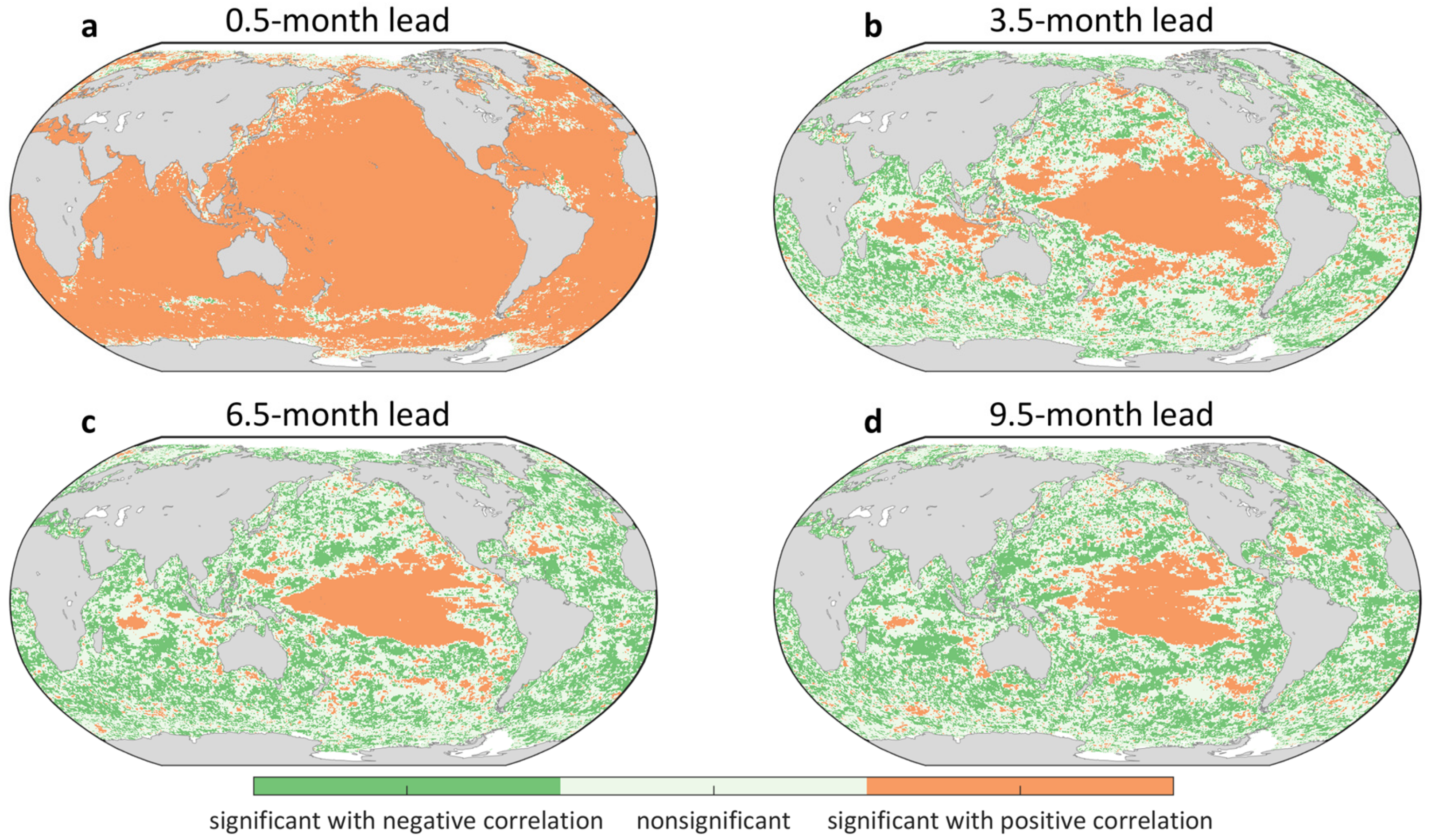
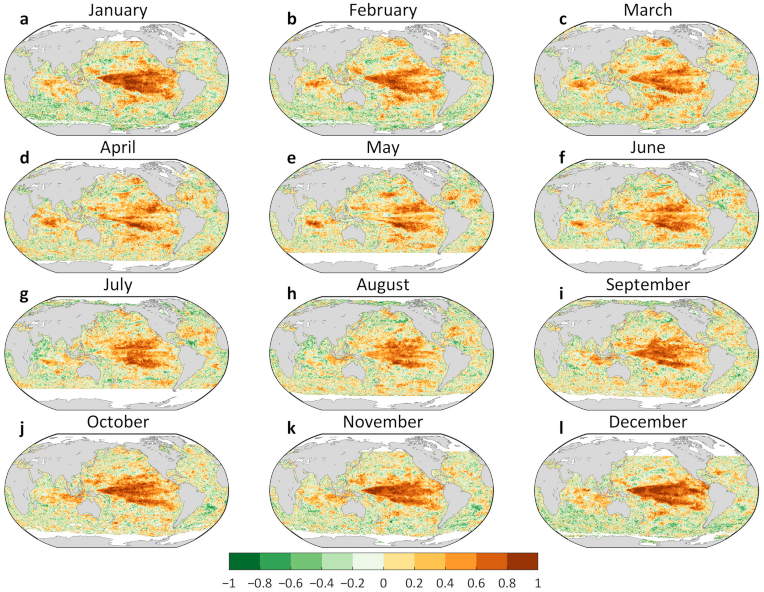
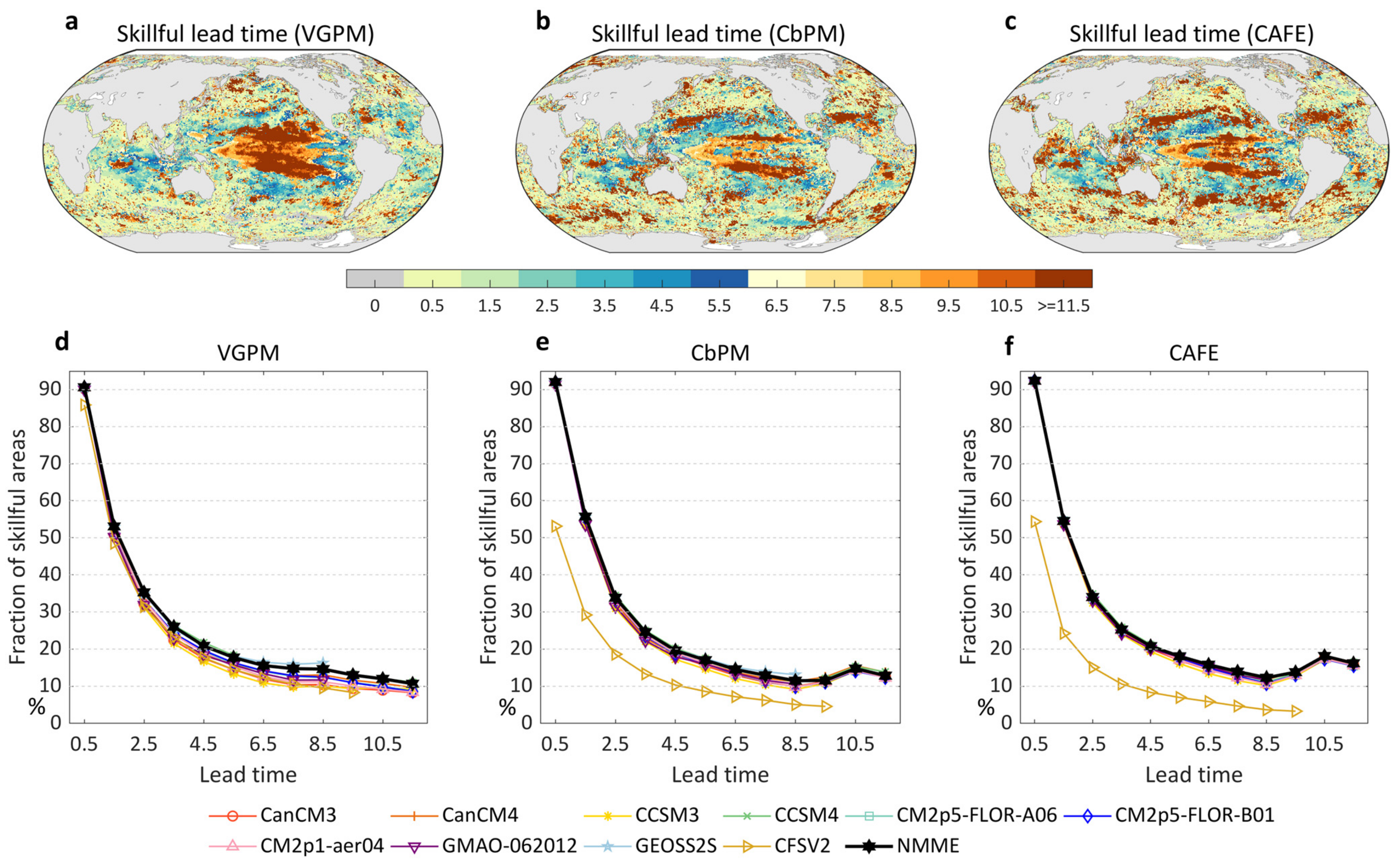
3.2. Spatiotemporal Patterns of Skillful Lead Time

Higher predictability is largely distributed over equatorial Pacific, equatorial Indian Ocean, North Atlantic and some scattered areas over the Pacific, South Atlantic, Indian Ocean and the Southern Ocean, with a skillful lead time more than 11.5 months (Figure 9a). The skillful areas are generally located at mid-low latitudes, which is related to nutrient and biomass advection and high SST predictability in these areas [7,8,52]. The ten heterogeneous NMME models show similar temporal patterns in terms of the fraction of skillful areas (Figure 9b), indicating a decreasing trend with the increase of lead time. There are ~90% and ~10% ocean NPP areas with significant forecasting skill at 0.5-month and 11.5-month lead times, respectively. The NMME model indicates some improvements over most of the heterogeneous models after equal weighting (Figure 9b), partly because the random biases and errors in each model are averaged to increase the signal-to-noise ratio [17,41]. Although the GEOSS2S and CCSM4 models demonstrate similar skill with NMME, the advantages of NMME relative to most of the involved models are evident from 0.5- to 11.5-month lead times. The advantage of multi-model ensemble is also highlighted in previous studies for precipitation forecasting [17], SST prediction [41] and wildfire forecasting [18]. It is not surprising that the averaged NMME may not always perform the best over all the lead times, due to the spatiotemporal heterogeneity of forecasting biases and gaps in each model. The increasing advances in climate and ocean models could further enhance the SST prediction and NPP forecasting skills [16].
There are some similarities and differences in the spatiotemporal patterns of forecasting skill using VGPM, CbPM and CAFÉ NPP datasets (Figure 10). The skillful areas are largely distributed over mid-low latitudes such as the equatorial Pacific and Indian oceans, and the skillful areas are generally consistent from 0.5- to 11.5-month leads for the three NPP datasets. For example, approximately 20% productive ocean areas demonstrate significant skills at 4.5-month lead time for each of the three datasets. However, the most skillful regions based on CbPM and CAFÉ datasets seem more scattered versus VGPM data, as the skillful areas at a 11.5-month lead time are distributed unevenly across many oceans (e.g., the Southern Ocean) for the former two NPP datasets. The differences of the spatial patterns of forecasting skill for the three NPP datasets are expected because they are retrieved with different algorithms and inputs [10,11,12], and the correlations between NPP and the used predictors exhibit different spatial patterns (Figure 11).

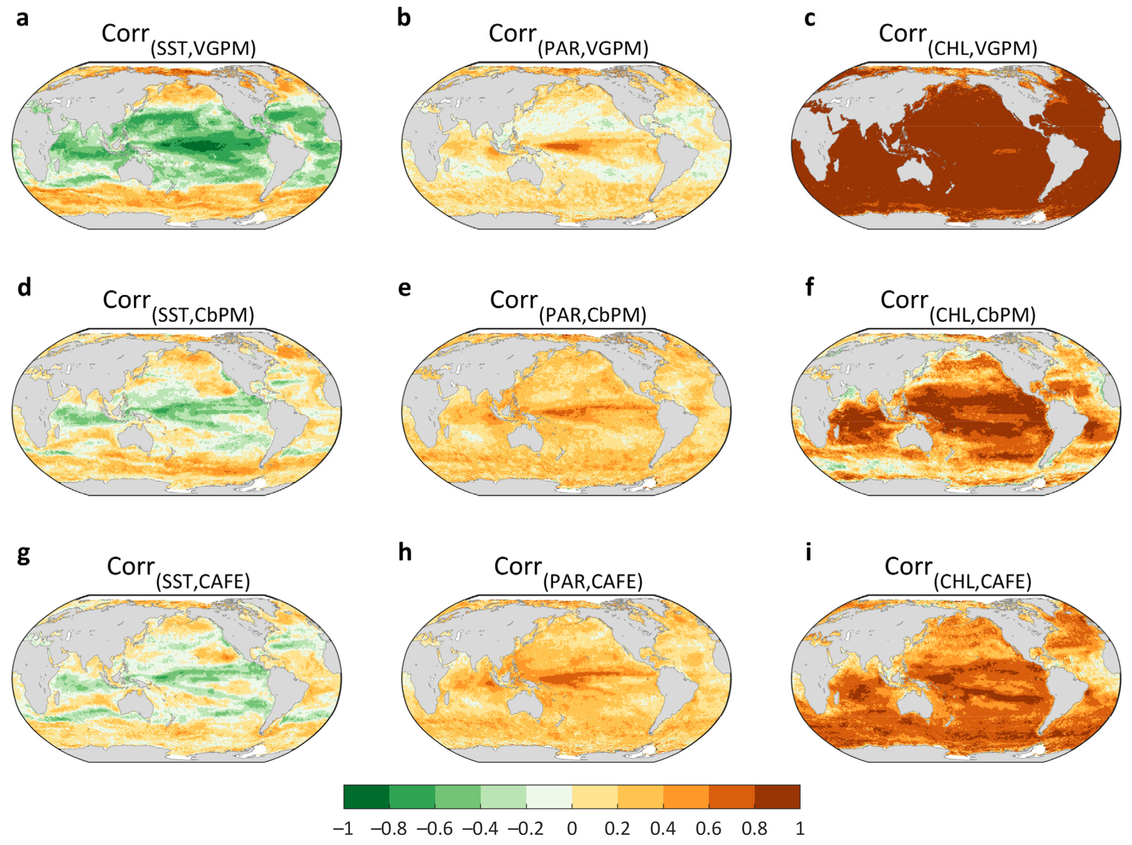
3.3. Attribution of the Forecasting Skill

Figure 12 presents the comparisons of the forecasting skill based on temporal memory, climate predictions and their combination in space and time. The combined forecasting improves the forecasting skill by NPP memory over many areas (Figure 12a), especially for the equatorial Pacific and Indian oceans. When all the temporal memories are considered in forecasting, the skill improvement for joint forecasting over memory is centralized over equatorial areas (Figure 12b), suggesting an added value of climate predictions versus temporal memory, consistent with the spatial pattern of the SST forecasting skill (Figure 13). The integrated forecasting shows substantial skill improvement versus solely climate predictions over numerous regions (Figure 12c), indicating the dominance of the memory information from historical data in NPP forecasting [8,13]. A spatial comparison of the absolute forecasting skills between individual and integrated predictions in space is presented in Figure 14. It is also found that the joint use of climate prediction and temporal memory may slightly degrade the forecasting skill for some small areas (Figure 12a–c), likely due to overfitting by including more predictors or the nonstationarity of predictor-predictand relationship [38,53,54,55].
The memory-based forecasting from NPP and chlorophyll dominates in the first several lead months, while the climate prediction is secondary (Figure 12). Approximately 90% (45%) and 29% (20%) of the productive areas are skillfully predicted (significant at 5% significance level) for memory-based (NMME_sst) model at 0.5 and 2.5 lead months, respectively. The memory-based prediction by NPP is superior to univariate forecasting using SST, PAR and CHL predictors and climate prediction from 0.5 to 3.5 lead months, but fails to outperform climate prediction (NMME_sst) from 4.5 to 9.5 lead months, suggesting a quick dropping rate of the forecasting skill in the former than the latter. Combining the memory of four predictors help improve the memory-based forecasting skill relative to the solely use of NPP predictor, because of long-term memories from SST and satellite-based chlorophyll [43,52,56]. For example, a ~4% increase of skillful areas is highlighted at 5.5-month lead for multivariate memory-based prediction (HisALL) versus NPP memory (HisNPP). The climate prediction complements the memory-based prediction by relating SST forecasting to NPP, especially at longer leads. An improvement of 5% skillful areas is expected by the joint use of temporal memory and climate prediction (Combined) versus memory-based prediction from 3.5 to 8.5 months (Figure 12d). The magnitudes of skill improvements for joint forecasting versus individual forecasting vary with three NPP datasets (Figure 15). The SST-based NPP predictions from NMME contribute limited skill improvement to memory-based forecasting for CbPM and CAFÉ versus VGPM datasets, because the VGPM NPP dataset exhibits a higher correlation with SST relative to CbPM and CAFÉ datasets in space (Figure 11).

3.4. The Uncertainty of the Forecasting Skill

We calculated the RMSE to represent the prediction error of ocean NPP forecasting (Figure 16). The prediction error is relatively larger over polar regions and the coastal regions versus other areas, which is possibly related to data uncertainty, sample size, NPP distribution and the model imperfection. The RMSE demonstrates similar spatial patterns over different lead times, and shows no obvious increase with lead time, suggesting the RMSE generally constrained within a specific range by the forecasting model. We also plotted the averaged RMSE and Bias (gC m−2 month−1) over the equatorial Pacific to see how the uncertainty changes over time (Figure 17). The averaged RMSE over the equatorial Pacific demonstrates an increasing trend with the increase of lead time, which is expected because the predictive error usually accumulates by time. The RMSE uncertainty is well controlled within a specific range and the bias uncertainty range includes zero for a few lead times while exceeds zero for 5- to 8-month leads, demonstrating the underlying potential for ocean forecasting while still having room for improvement.

4. Discussion

Ocean productivity forecasting is a challenging issue due to complex physical and biogeochemical interactions of underlying drivers and uncertainties in data and models [8,13,14]. The NPP predictability is explored here by combining climate predictions and temporal memory information at seasonal scales over global oceans. Compared with previous studies [7,8,14], we innovatively integrate the state-of-the-art climate predictions and the long-term memory from historical data in a regression-based model to improve ocean productivity predictability. Substantial areas are expected to be predictable for several months in advance, although the forecasting skill varies with climate models and NPP data [10,11,12,17]. The SST predictability at longer leads contributes to the skill improvement of NPP forecasting largely over the tropics, and this contribution is likely to increase with the advance of horizon and time of SST predictability [52,56]. The NPP forecasting skill comes mainly from temporal memory of chlorophyll and productivity over extratropical oceans, which is related to local persistence of nutrient anomalies, advection and the possible propagation of climate modes on biome boundaries [7,8,13,14], such as ENSO. Further improvement of NPP predictability over extratropical oceans requires a deep understanding and modeling of the advection pattern, reemergence, the remote effect of climate modes and the new predictability sources such as sea surface salinity and sea ice process [14].
The predictive skills greatly improved as shown by the developed forecasting model versus productivity persistence and the skillfully predicted areas increase by ~10% (from 5% to 15%) over global oceans at 6.5-month lead. The substantial improvement demonstrates the effectiveness of the developed model by combining climate predictions and temporal memories. The skill improvement is related to two major refinements: the inclusion of multifactor memories and the integration of climate predictions. The skillfully predicted areas increase by ~5% after including the multifactor memories at 6.5-month lead and by another ~5% by adding the climate predictions further. Therefore, the multifactor temporal memories and the climate predictions contribute equally to the skills at this lead, highlighting the importance of the two new strategies. For the temporal memories, the contributions are relatively less at shorter leads and more at longer leads, which may be explained by the high persistence at smaller lead times. The contribution of climate predictions demonstrates similar trend with multifactor memories, suggesting great potential for long-lead ocean condition prediction by climate models.
The ten NMME models demonstrate similar performance and vary from model to model. For example, a ~8% skill improvement is seen for GEOSS2S model versus CFSV2 at 8.5-month lead, which is related to their differences in model structure, parameters and prediction process. With the advance of numerical climate models, the SST predictability can be further expanded [16,39]. Apart from the numerical models, the heuristic machine learning or deep learning methods provide strong predictive capability of SST [52,57,58], such as convolutional neural network (CNN) or recurrent neural network (RNN). The SST predictions by deep learning models can also be incorporated into the developed forecasting model. The ensemble mean of the ten models demonstrate superior performance versus most of individual models, highlighting the benefit of ensemble forecasting, which is consistent with previous studies [22,39,40,41].
The proposed joint forecasting model is a flexible framework and much more predictors can be adaptively included, such as nutrient and biome, when data are available. Currently, the SST, CHL, PAR and NPP are included as predictors and this may not be enough to capture the complex long-term dependences between ocean productivity and its influential factors. The stratification, upwelling and vertical mixing are also potential predictors for dynamic integration into the forecasting model [59,60,61]. The regression-based framework is a simple but effective way to incorporate new predictability sources without tremendous increase of calculation effort. Although the used predictors may not cover all the important predictability sources, significant improvements are shown in the joint forecasting model versus productivity persistence. It is expected that the predictive skills would be further improved when suitable predictability sources are incorporated.
The predictive performances using three NPP data demonstrate similar but different spatiotemporal patterns. For the VGPM NPP data, the SST is a key variable for deriving the physiological variability parameter based on daily integrated production measurements (Pb_opt) [10]. The SST variable is not considered in CbPM NPP data [11] and is used to get the backscattering by pure water parameter in CAFÉ NPP [12]. Therefore, it is expected that the contributions of NMME to the joint forecasting model for CbPM and CAFÉ NPP data may not be as high as that of VGPM NPP. However, the joint forecasting model could still demonstrate some improvements over productivity persistence, which is appealing for the ocean productivity forecasting.
The regression-based forecasting model captures the linear dependence between NPP and its predictors explicitly and can prevent overfitting versus extremely complex models [15,18]. However, the relationship between NPP and its drivers is natively nonlinear and the linear regression method may be insufficient to extract high-level features from the data. Therefore, the predictability may be further improved by incorporating sophisticated deep learning methods to learn nonlinear plausible features from massive data [43,52]. A limitation of this study is the neglect of nonstationarity of the predictor–predictand relationship over space and time [62,63], which will weaken the robustness and generalization of out-of-sample forecasting skill. The predictor-predictand relationship is assumed to be unchanged during the study period, which is not practically true because climate change is shifting the patterns of ocean cycle [64,65,66]. Therefore, the dynamic integration of statistical or heuristic and process-based biogeochemical models may shed new light on the improvement of NPP predictability in the ocean [23,26,27,28,67].
The uncertainties of the developed model are related to the uncertainties in data and the used predictors. Specifically, the uncertainties come from measurement, representation, and prediction errors [68]. The measurement error is the potential systematic and random errors from data retrieval and sampling. The NPP data may not be precise due to the measurement error and the retrieval algorithm and this uncertainty can be partly estimated using triple collocation method or in-situ validation [69]. The representation error exists when the spatial resolutions between the grid observation and the in-situ samples mismatch. The in-situ phytoplankton data used for validation may not be representative of the 0.5° × 0.5° grids used in prediction and the representative error can be estimated by comparing the grid observations with enough in-situ samples within a grid cell [70]. The prediction errors are related to the evaluation of the statistical model using independent test data, such as the evaluations using RMSE and Bias. The three types of errors may be correlated with each other as the measurement error may be propagated into parameters and then the prediction errors. For simplicity, here we only estimate the prediction errors based on RMSE and Bias statistics. The remote sensing-based NPP datasets demonstrate some differences in the predictive skills spatiotemporally. The uncertainties in predictor data such as SST and PAR may also bring uncertainty into the model. Therefore, accurate retrieval of ocean and biophysical parameters are critical for the improvement of predictive accuracy. On the other hand, new predictability factors, such as the phytoplankton community composition, upwelling, salinity and nutrient, may be well incorporated into the forecasting model to enhance the predictive skill. As for the model itself, attention should be paid to the overfitting problem and the important predictors should be selected to avoid overselection.
The ocean NPP or chlorophyll forecasting is generally conducted by statistical or physically-based models. The Ocean Biogeochemical Model (NOBM) achieves an anomaly correlation coefficient (ACC) of 0.33 and 0.15 for 1-month and 6-month chlorophyll forecasting over the equatorial Pacific [71], which is lower than our skill in Figure 2 (0.50 and 0.22 at 1.5-month and 6.5-month leads, respectively, averaged over the equatorial Pacific). Another model-based prediction shows an ACC value of 0.09 for chlorophyll forecasting over the equatorial Pacific at 9-month lead [72], while our skill is 0.15 at this lead, suggesting an added value of the developed model. Given the strong correlations (close to 1) between chlorophyll and NPP in Figure 11 for VGPM NPP, the predictive skills for NPP and CHL are comparable. A previous study demonstrated that more than 50% areas of the equatorial Pacific cannot achieve an ACC of 0.1 in practice for NPP forecasting [8], while our model suggests that ~66% of the equatorial Pacific have an ACC larger than 0.1. Therefore, the developed joint forecasting model is effective in improving the accuracy of NPP prediction.
The R2 value between in-situ data and grid-based NPP is 0.51 over the tropical oceans. Given the sparse characteristic of the distribution of in-situ phytoplankton data, the results are expected due to the limited sample size (245) and the representation error between in-situ data and remote sensing productivity data. In fact, we could not find any relevant literature that uses the very sparse in-situ phytoplankton data for validation of grid-based prediction. It would be more convincing if there are enough spatially evenly-distributed in-situ samples for validating the grid-based prediction. However, it is difficult to judge how the model performs over the vast oceans for now, while it could be concluded that the R2 value by in-situ validation of grid-based forecasting does not deviate away from that of the value between in-situ data and observed gridded data over the available point locations. We then compare the developed model with the persistence-based baseline model, in terms of the R2 value in NPP forecasting. The persistence-based model is used in previous studies for NPP forecasting, which assumes the observation in previous time steps as prediction. The R2 value for the persistence-based model is 0.40 and 0.07 for 1-month and 10-month lead, respectively, which is worse than our developed model (0.52 and 0.47 for 1-month and 10-month leads, respectively). Therefore, it is likely that the developed forecasting model is better than the persistence-based baseline model for NPP forecasting, in terms of the in-situ validation over the tropical oceans.
Compared with previous studies [7,8,13], this study not only highlights the promising predictive skills over the equatorial Pacific and Indian oceans, but also demonstrates the added values of ensemble climate prediction and multi-factor memories over persistence, which may provide new insights into further improvement of phytoplankton productivity forecasting. This study focuses on the joint use of climate prediction and multi-factor memories for NPP forecasting and highlights the complemental roles of the two forecasting parts, which is generally lacking in existing studies [7,8,26]. This study also reveals the spatiotemporal patterns of the predictive skills for different lead times, seasons and datasets, which provides a relatively complete depiction of phytoplankton productivity predictability. As this experiment is conducted over global oceans, the spatial resolution of productivity forecasting may be lower relative to those of local and coastal studies [4,14]. In addition, the regression-based forecasting model may also be further refined by some machine learning methods with parameter optimization [32,34,35].

5. Conclusions

In this study, we propose an integrated model for ocean productivity forecasting by joint use of seasonal climate predictions and temporal memory information from historical months. The developed model combines the SST predictions from NMME and memory-based predictors to predict ocean productivity in a regression model. Compared with individual predictions, the joint forecasting absorbs the strengths from the temporal similarity and propagation of time series and the dynamic simulations of SST from atmosphere-ocean models. The memory-based information provides the predictability over many extratropical oceans and the dynamic SST predictions enhances the predictability over equatorial oceans. Therefore, the subtle integration of data-driven and model-driven predictions suggests promising potential for hybrid ocean productivity forecasting for a couple of months in advance.
In the joint forecasting model, the SST predictions from climate models are used as predictors to integrate with multifactor memories in NPP forecasting. In fact, the biogeochemical models driven with climate forecasts can also be directly integrated into the joint forecasting model together with temporal memory. The physically-based biogeochemical models have advantages in subtle process modeling and is appealing for long-term extrapolation with the advances of observations, model representation and data assimilation techniques [73,74,75,76]. Further, the new predictability sources, such as the light distribution, upwelling, mixed layer depth, biome activity, etc., can be flexibly incorporated into the forecasting model when the relevant data are available. Therefore, it would be expected that the ocean productivity predictability would be gradually improved with the development of data and models.
This research has some limitations which need to be further resolved in the future. First, only the SST, CHL, PAR and NPP data are utilized as predictors and much more predictors should be incorporated such as the MLD, light, nutrient and biome distribution. The predictive skills of the joint forecasting model would further be refined by including more factors. Second, the predictive skills at longer lead time decrease quickly at some extratropical regions, which need to be paid much attention. Although the extratropical predictability may not be as high as that of tropical areas, the extratropical prediction would be improved by elaborate modeling of underlying key driving factors.

Author Contributions

Conceptualization, L.X.; methodology, L.X.; formal analysis, L.X.; writing—original draft preparation, L.X.; writing—review and editing, L.X., H.Y., Z.C., W.D., N.C. and C.Z.; supervision, L.X.; funding acquisition, L.X. and H.Y. All authors have read and agreed to the published version of the manuscript.

Funding

This research was supported by the National Natural Science Foundation of China (42201509, 42101429), the National Key Research and Development Program for Young Scientist (2021YFF0704400), the Fundamental Research Funds for the Central Universities, China University of Geosciences (Wuhan) (162301212687, 2642022009) and the Special Fund of Hubei Luojia Laboratory (220100034).

Data Availability Statement

All of the used data in this work are publicly available from their official sites. The VGPM, CbPM and CAFÉ NPP datasets and their ancillary inputs are available from http://sites.science.oregonstate.edu/ocean.productivity/index.php, accessed on 25 October 2022. The NMME predictions are available from the International Research Institute for Climate and Society (IRI) data library website (https://iridl.ldeo.columbia.edu/SOURCES/.Models/.NMME/, accessed on 3 November 2022). The processed data and results are available for interested readers upon request from the corresponding author. The programming codes for processing the data and analyzing the results are available upon reasonable request from the corresponding author. The data processing, analysis and plotting codes are written based on MATLAB Version 9.4 (R2018a). The MATLAB product is available from https://www.mathworks.com/products/matlab.html, accessed on 18 October 2022.

Conflicts of Interest

The authors declare no conflict of interest.

References

  1. Field, C.B.; Behrenfeld, M.J.; Randerson, J.T.; Falkowski, P. Primary production of the biosphere: Integrating terrestrial and oceanic components. Science 1998, 281, 237–240. [Google Scholar] [CrossRef] [PubMed] [Green Version]
  2. Boyd, P.W.; Sundby, S.; Pörtner, H.-O. Cross-chapter box on net primary production in the ocean. In Climate Change 2014: Impacts, Adaptation, and Vulnerability. Part A: Global and Sectoral Aspects. Contribution of Working Group II to the Fifth Assessment Report of the Intergovernmental Panel of Climate Change; Cambridge University Press: Cambridge, UK, 2014; pp. 133–136. [Google Scholar]
  3. Sigman, D.M.; Hain, M.P. The biological productivity of the ocean. Nat. Educ. Knowl. 2012, 3, 21. [Google Scholar]
  4. Stock, C.A.; John, J.G.; Rykaczewski, R.R.; Asch, R.G.; Cheung, W.W.; Dunne, J.P.; Friedland, K.D.; Lam, V.W.; Sarmiento, J.L.; Watson, R.A. Reconciling fisheries catch and ocean productivity. Proc. Natl. Acad. Sci. USA 2017, 114, E1441–E1449. [Google Scholar] [CrossRef] [PubMed] [Green Version]
  5. Moore, J.K.; Fu, W.; Primeau, F.; Britten, G.L.; Lindsay, K.; Long, M.; Doney, S.C.; Mahowald, N.; Hoffman, F.; Randerson, J.T. Sustained climate warming drives declining marine biological productivity. Science 2018, 359, 1139–1143. [Google Scholar] [CrossRef] [Green Version]
  6. Brander, K.M. Global fish production and climate change. Proc. Natl. Acad. Sci. USA 2007, 104, 19709–19714. [Google Scholar] [CrossRef] [Green Version]
  7. Krumhardt, K.M.; Lovenduski, N.S.; Long, M.C.; Luo, J.; Lindsay, K.; Yeager, S.; Harrison, C. Potential predictability of net primary production in the ocean. Glob. Biogeochem. Cycles 2020, 34, e2020GB006531. [Google Scholar] [CrossRef]
  8. Taboada, F.G.; Barton, A.D.; Stock, C.A.; Dunne, J.; John, J.G. Seasonal to interannual predictability of oceanic net primary production inferred from satellite observations. Prog. Oceanogr. 2019, 170, 28–39. [Google Scholar] [CrossRef]
  9. Pitcher, G.; Figueiras, F.; Hickey, B.; Moita, M. The physical oceanography of upwelling systems and the development of harmful algal blooms. Prog. Oceanogr. 2010, 85, 5–32. [Google Scholar] [CrossRef] [Green Version]
  10. Behrenfeld, M.J.; Falkowski, P.G. Photosynthetic rates derived from satellite-based chlorophyll concentration. Limnol. Oceanogr. 1997, 42, 1–20. [Google Scholar] [CrossRef]
  11. Westberry, T.; Behrenfeld, M.; Siegel, D.; Boss, E. Carbon-based primary productivity modeling with vertically resolved photoacclimation. Glob. Biogeochem. Cycles 2008, 22, 3078. [Google Scholar] [CrossRef] [Green Version]
  12. Silsbe, G.M.; Behrenfeld, M.J.; Halsey, K.H.; Milligan, A.J.; Westberry, T.K. The CAFE model: A net production model for global ocean phytoplankton. Glob. Biogeochem. Cycles 2016, 30, 1756–1777. [Google Scholar] [CrossRef]
  13. Séférian, R.; Bopp, L.; Gehlen, M.; Swingedouw, D.; Mignot, J.; Guilyardi, E.; Servonnat, J. Multiyear predictability of tropical marine productivity. Proc. Natl. Acad. Sci. USA 2014, 111, 11646–11651. [Google Scholar] [CrossRef] [PubMed] [Green Version]
  14. Jacox, M.G.; Alexander, M.A.; Siedlecki, S.; Chen, K.; Kwon, Y.-O.; Brodie, S.; Ortiz, I.; Tommasi, D.; Widlansky, M.J.; Barrie, D.; et al. Seasonal-to-interannual prediction of North American coastal marine ecosystems: Forecast methods, mechanisms of predictability, and priority developments. Prog. Oceanogr. 2020, 183, 102307. [Google Scholar] [CrossRef]
  15. Tian, S.; Van Dijk, A.I.; Tregoning, P.; Renzullo, L.J. Forecasting dryland vegetation condition months in advance through satellite data assimilation. Nat. Commun. 2019, 10, 469. [Google Scholar] [CrossRef] [PubMed] [Green Version]
  16. Lee, E.; Koster, R.D.; Ott, L.E.; Joiner, J.; Zeng, F.-W.; Kolassa, J.; Reichle, R.H.; Arsenault, K.R.; Hazra, A.; Shukla, S. Skillful Seasonal Forecasts of Land Carbon Uptake in Northern Mid- and High Latitudes. Geophys. Res. Lett. 2022, 49, e2021GL097117. [Google Scholar] [CrossRef]
  17. Kirtman, B.P.; Min, D.; Infanti, J.M.; Kinter, J.L.; Paolino, D.A.; Zhang, Q.; Van Den Dool, H.; Saha, S.; Mendez, M.P.; Becker, E. The North American multimodel ensemble: Phase-1 seasonal-to-interannual prediction; phase-2 toward developing intraseasonal prediction. Bull. Am. Meteorol. Soc. 2014, 95, 585–601. [Google Scholar] [CrossRef] [Green Version]
  18. Turco, M.; Jerez, S.; Doblas-Reyes, F.J.; AghaKouchak, A.; Llasat, M.C.; Provenzale, A. Skilful forecasting of global fire activity using seasonal climate predictions. Nat. Commun. 2018, 9, 1–9. [Google Scholar] [CrossRef] [PubMed] [Green Version]
  19. Jacox, M.G.; Alexander, M.A.; Amaya, D.; Becker, E.; Bograd, S.J.; Brodie, S.; Hazen, E.L.; Pozo Buil, M.; Tommasi, D. Global seasonal forecasts of marine heatwaves. Nature 2022, 604, 486–490. [Google Scholar] [CrossRef]
  20. Gregg, W.W. Tracking the SeaWiFS record with a coupled physical/biogeochemical/radiative model of the global oceans. Deep. Sea Res. Part II Top. Stud. Oceanogr. 2001, 49, 81–105. [Google Scholar] [CrossRef]
  21. Thiboult, A.; Anctil, F.; Boucher, M.-A. Accounting for three sources of uncertainty in ensemble hydrological forecasting. Hydrol. Earth Syst. Sci. 2016, 20, 1809–1825. [Google Scholar] [CrossRef] [Green Version]
  22. Tebaldi, C.; Knutti, R. The use of the multi-model ensemble in probabilistic climate projections. Philos. Trans. R. Soc. A: Math. Phys. Eng. Sci. 2007, 365, 2053–2075. [Google Scholar] [CrossRef] [PubMed]
  23. Xu, L.; Chen, N.; Chen, Z.; Zhang, C.; Yu, H. Spatiotemporal forecasting in earth system science: Methods, uncertainties, predictability and future directions. Earth Sci. Rev. 2021, 222, 103828. [Google Scholar] [CrossRef]
  24. Xu, L.; Chen, N.; Zhang, X.; Chen, Z. A data-driven multi-model ensemble for deterministic and probabilistic precipitation forecasting at seasonal scale. Clim. Dyn. 2020, 54, 3355–3374. [Google Scholar] [CrossRef]
  25. Yuan, X.; Wood, E.F. Multimodel seasonal forecasting of global drought onset. Geophys. Res. Lett. 2013, 40, 4900–4905. [Google Scholar] [CrossRef]
  26. Irrgang, C.; Boers, N.; Sonnewald, M.; Barnes, E.A.; Kadow, C.; Staneva, J.; Saynisch-Wagner, J. Towards neural Earth system modelling by integrating artificial intelligence in Earth system science. Nat. Mach. Intell. 2021, 3, 667–674. [Google Scholar] [CrossRef]
  27. AghaKouchak, A.; Pan, B.; Mazdiyasni, O.; Sadegh, M.; Jiwa, S.; Zhang, W.; Love, C.; Madadgar, S.; Papalexiou, S.; Davis, S. Status and prospects for drought forecasting: Opportunities in artificial intelligence and hybrid physical–statistical forecasting. Philos. Trans. R. Soc. A 2022, 380, 20210288. [Google Scholar] [CrossRef]
  28. Slater, L.; Arnal, L.; Boucher, M.-A.; Chang, A.Y.-Y.; Moulds, S.; Murphy, C.; Nearing, G.; Shalev, G.; Shen, C.; Speight, L. Hybrid forecasting: Using statistics and machine learning to integrate predictions from dynamical models. Hydrol. Earth Syst. Sci. Discuss. 2022, preprint. [Google Scholar]
  29. Xu, L.; Chen, N.; Zhang, X.; Chen, Z. An evaluation of statistical, NMME and hybrid models for drought prediction in China. J. Hydrol. 2018, 566, 235–249. [Google Scholar] [CrossRef] [Green Version]
  30. Adnan, R.M.; Mostafa, R.R.; Kisi, O.; Yaseen, Z.M.; Shahid, S.; Zounemat-Kermani, M. Improving streamflow prediction using a new hybrid ELM model combined with hybrid particle swarm optimization and grey wolf optimization. Knowl. Based Syst. 2021, 230, 107379. [Google Scholar] [CrossRef]
  31. Adnan, R.M.; Kisi, O.; Mostafa, R.R.; Ahmed, A.N.; El-Shafie, A. The potential of a novel support vector machine trained with modified mayfly optimization algorithm for streamflow prediction. Hydrol. Sci. J. 2022, 67, 161–174. [Google Scholar] [CrossRef]
  32. Adnan, R.M.; Mostafa, R.R.; Elbeltagi, A.; Yaseen, Z.M.; Shahid, S.; Kisi, O. Development of new machine learning model for streamflow prediction: Case studies in Pakistan. Stoch. Environ. Res. Risk Assess. 2022, 36, 999–1033. [Google Scholar] [CrossRef]
  33. Ikram, R.M.A.; Ewees, A.A.; Parmar, K.S.; Yaseen, Z.M.; Shahid, S.; Kisi, O. The viability of extended marine predators algorithm-based artificial neural networks for streamflow prediction. Appl. Soft Comput. 2022, 131, 109739. [Google Scholar] [CrossRef]
  34. Ikram, R.M.A.; Dai, H.-L.; Al-Bahrani, M.; Mamlooki, M. Prediction of the FRP Reinforced Concrete Beam shear capacity by using ELM-CRFOA. Measurement 2022, 205, 112230. [Google Scholar] [CrossRef]
  35. Espeholt, L.; Agrawal, S.; Sønderby, C.; Kumar, M.; Heek, J.; Bromberg, C.; Gazen, C.; Carver, R.; Andrychowicz, M.; Hickey, J.; et al. Deep learning for twelve hour precipitation forecasts. Nat. Commun. 2022, 13, 5145. [Google Scholar] [CrossRef]
  36. Xiao, C.; Chen, N.; Hu, C.; Wang, K.; Xu, Z.; Cai, Y.; Xu, L.; Chen, Z.; Gong, J. A spatiotemporal deep learning model for sea surface temperature field prediction using time-series satellite data. Environ. Model. Softw. 2019, 120, 104502. [Google Scholar] [CrossRef]
  37. Xu, L.; Chen, N.; Zhang, X.; Chen, Z.; Hu, C.; Wang, C. Improving the North American multi-model ensemble (NMME) precipitation forecasts at local areas using wavelet and machine learning. Clim. Dyn. 2019, 53, 601–615. [Google Scholar] [CrossRef]
  38. Liu, T.; Schmitt, R.W.; Li, L. Global Search for Autumn-Lead Sea Surface Salinity Predictors of Winter Precipitation in Southwestern United States. Geophys. Res. Lett. 2018, 45, 8445–8454. [Google Scholar] [CrossRef]
  39. Becker, E.J.; Kirtman, B.P.; L’Heureux, M.; Muñoz, Á.G.; Pegion, K. A Decade of the North American Multimodel Ensemble (NMME): Research, Application, and Future Directions. Bull. Am. Meteorol. Soc. 2022, 103, E973–E995. [Google Scholar] [CrossRef]
  40. Roy, T.; He, X.; Lin, P.; Beck, H.E.; Castro, C.; Wood, E.F. Global evaluation of seasonal precipitation and temperature forecasts from NMME. J. Hydrometeorol. 2020, 21, 2473–2486. [Google Scholar] [CrossRef]
  41. Becker, E.; den Dool, H.v.; Zhang, Q. Predictability and Forecast Skill in NMME. J. Clim. 2014, 27, 5891–5906. [Google Scholar] [CrossRef]
  42. Shin, S.-I.; Newman, M. Seasonal Predictability of Global and North American Coastal Sea Surface Temperature and Height Anomalies. Geophys. Res. Lett. 2021, 48, e2020GL091886. [Google Scholar] [CrossRef]
  43. Na, L.; Shaoyang, C.; Zhenyan, C.; Xing, W.; Yun, X.; Li, X.; Yanwei, G.; Tingting, W.; Xuefeng, Z.; Siqi, L. Long-term prediction of sea surface chlorophyll-a concentration based on the combination of spatio-temporal features. Water Res. 2022, 211, 118040. [Google Scholar] [CrossRef] [PubMed]
  44. Justice, C.O.; Vermote, E.; Townshend, J.R.; Defries, R.; Roy, D.P.; Hall, D.K.; Salomonson, V.V.; Privette, J.L.; Riggs, G.; Strahler, A. The Moderate Resolution Imaging Spectroradiometer (MODIS): Land remote sensing for global change research. IEEE Trans. Geosci. Remote Sens. 1998, 36, 1228–1249. [Google Scholar] [CrossRef] [Green Version]
  45. Mattei, F.; Scardi, M. Collection and analysis of a global marine phytoplankton primary-production dataset. Earth Syst. Sci. Data 2021, 13, 4967–4985. [Google Scholar] [CrossRef]
  46. Harnos, D.S.; Schemm, J.-K.E.; Wang, H.; Finan, C.A. NMME-based hybrid prediction of Atlantic hurricane season activity. Clim. Dyn. 2019, 53, 7267–7285. [Google Scholar] [CrossRef]
  47. Zhang, W.; Villarini, G.; Slater, L.; Vecchi, G.A.; Bradley, A.A. Improved ENSO forecasting using bayesian updating and the North American multimodel ensemble (NMME). J. Clim. 2017, 30, 9007–9025. [Google Scholar] [CrossRef]
  48. Li, H.; Sheffield, J.; Wood, E.F. Bias correction of monthly precipitation and temperature fields from Intergovernmental Panel on Climate Change AR4 models using equidistant quantile matching. J. Geophys. Res. Atmos. 2010, 115, 12882. [Google Scholar] [CrossRef]
  49. Bett, P.E.; Williams, K.E.; Burton, C.; Scaife, A.A.; Wiltshire, A.J.; Gilham, R. Skillful seasonal prediction of key carbon cycle components: NPP and fire risk. Environ. Res. Commun. 2020, 2, 055002. [Google Scholar] [CrossRef]
  50. Smith, A.; Atkinson, N.; Bell, W.; Doherty, A. An initial assessment of observations from the Suomi-NPP satellite: Data from the Cross-track Infrared Sounder (CrIS). Atmos. Sci. Lett. 2015, 16, 260–266. [Google Scholar] [CrossRef]
  51. Kostenko, A.V.; Hyndman, R.J. Forecasting without Significance Tests? Monash University: Melbourne, Australia, 2008. [Google Scholar]
  52. Ham, Y.-G.; Kim, J.-H.; Luo, J.-J. Deep learning for multi-year ENSO forecasts. Nature 2019, 573, 568–572. [Google Scholar] [CrossRef]
  53. Bartlett, P.L.; Long, P.M.; Lugosi, G.; Tsigler, A. Benign overfitting in linear regression. Proc. Natl. Acad. Sci. USA 2020, 117, 30063–30070. [Google Scholar] [CrossRef] [PubMed] [Green Version]
  54. Sahai, A.; Chattopadhyay, R.; Goswami, B.N. A SST based large multi-model ensemble forecasting system for Indian summer monsoon rainfall. Geophys. Res. Lett. 2008, 35, 35461. [Google Scholar] [CrossRef] [Green Version]
  55. Schmith, T. Stationarity of regression relationships: Application to empirical downscaling. J. Clim. 2008, 21, 4529–4537. [Google Scholar] [CrossRef]
  56. Newman, M.; Sardeshmukh, P.D. Are we near the predictability limit of tropical Indo-Pacific sea surface temperatures? Geophys. Res. Lett. 2017, 44, 8520–8529. [Google Scholar] [CrossRef]
  57. Liu, J.; Tang, Y.; Wu, Y.; Li, T.; Wang, Q.; Chen, D. Forecasting the Indian Ocean Dipole with deep learning techniques. Geophys. Res. Lett. 2021, 48, e2021GL094407. [Google Scholar] [CrossRef]
  58. Zheng, G.; Li, X.; Zhang, R.-H.; Liu, B. Purely satellite data–driven deep learning forecast of complicated tropical instability waves. Sci. Adv. 2020, 6, eaba1482. [Google Scholar] [CrossRef]
  59. Slagstad, D.; Wassmann, P.F.; Ellingsen, I. Physical constrains and productivity in the future Arctic Ocean. Front. Mar. Sci. 2015, 2, 85. [Google Scholar] [CrossRef] [Green Version]
  60. He, J.; Mahadevan, A. How the source depth of coastal upwelling relates to stratification and wind. J. Geophys. Res. Ocean. 2021, 126, e2021JC017621. [Google Scholar] [CrossRef]
  61. Randelhoff, A.; Sundfjord, A. Short commentary on marine productivity at Arctic shelf breaks: Upwelling, advection and vertical mixing. Ocean Sci. 2018, 14, 293–300. [Google Scholar] [CrossRef] [Green Version]
  62. Wang, Y.; Zhang, J.; Zhu, H.; Long, M.; Wang, J.; Yu, P.S. Memory in memory: A predictive neural network for learning higher-order non-stationarity from spatiotemporal dynamics. In Proceedings of the IEEE/CVF Conference on Computer Vision and Pattern Recognition, Long Beach, CA, USA, 15–20 June 2019; pp. 9154–9162. [Google Scholar]
  63. Slater, L.J.; Anderson, B.; Buechel, M.; Dadson, S.; Han, S.; Harrigan, S.; Kelder, T.; Kowal, K.; Lees, T.; Matthews, T. Nonstationary weather and water extremes: A review of methods for their detection, attribution, and management. Hydrol. Earth Syst. Sci. 2021, 25, 3897–3935. [Google Scholar] [CrossRef]
  64. Perry, A.L.; Low, P.J.; Ellis, J.R.; Reynolds, J.D. Climate change and distribution shifts in marine fishes. Science 2005, 308, 1912–1915. [Google Scholar] [CrossRef] [PubMed]
  65. Barton, A.D.; Irwin, A.J.; Finkel, Z.V.; Stock, C.A. Anthropogenic climate change drives shift and shuffle in North Atlantic phytoplankton communities. Proc. Natl. Acad. Sci. USA 2016, 113, 2964–2969. [Google Scholar] [CrossRef] [PubMed] [Green Version]
  66. Doney, S.C.; Ruckelshaus, M.; Emmett Duffy, J.; Barry, J.P.; Chan, F.; English, C.A.; Galindo, H.M.; Grebmeier, J.M.; Hollowed, A.B.; Knowlton, N. Climate change impacts on marine ecosystems. Annu. Rev. Mar. Sci. 2012, 4, 11–37. [Google Scholar] [CrossRef] [Green Version]
  67. Reichstein, M.; Camps-Valls, G.; Stevens, B.; Jung, M.; Denzler, J.; Carvalhais, N. Deep learning and process understanding for data-driven Earth system science. Nature 2019, 566, 195–204. [Google Scholar] [CrossRef]
  68. Gregor, L.; Gruber, N. OceanSODA-ETHZ: A global gridded data set of the surface ocean carbonate system for seasonal to decadal studies of ocean acidification. Earth Syst. Sci. Data 2021, 13, 777–808. [Google Scholar] [CrossRef]
  69. Xu, L.; Chen, N.; Zhang, X.; Moradkhani, H.; Zhang, C.; Hu, C. In-situ and triple-collocation based evaluations of eight global root zone soil moisture products. Remote. Sens. Environ. 2021, 254, 112248. [Google Scholar] [CrossRef]
  70. Xu, L.; Abbaszadeh, P.; Moradkhani, H.; Chen, N.; Zhang, X. Continental drought monitoring using satellite soil moisture, data assimilation and an integrated drought index. Remote. Sens. Environ. 2020, 250, 112028. [Google Scholar] [CrossRef]
  71. Rousseaux, C.S.; Gregg, W.W. Forecasting ocean chlorophyll in the Equatorial Pacific. Front. Mar. Sci. 2017, 4, 236. [Google Scholar] [CrossRef] [Green Version]
  72. Rousseaux, C.S.; Gregg, W.W.; Ott, L. Assessing the Skills of a Seasonal Forecast of Chlorophyll in the Global Pelagic Oceans. Remote. Sens. 2021, 13, 1051. [Google Scholar] [CrossRef]
  73. Castro de la Guardia, L.; Garcia-Quintana, Y.; Claret, M.; Hu, X.; Galbraith, E.; Myers, P. Assessing the role of high-frequency winds and sea ice loss on Arctic phytoplankton blooms in an ice-ocean-biogeochemical model. J. Geophys. Res. Biogeosciences 2019, 124, 2728–2750. [Google Scholar] [CrossRef]
  74. Schourup-Kristensen, V.; Sidorenko, D.; Wolf-Gladrow, D.A.; Völker, C. A skill assessment of the biogeochemical model REcoM2 coupled to the Finite Element Sea Ice–Ocean Model (FESOM 1.3). Geosci. Model Dev. 2014, 7, 2769–2802. [Google Scholar] [CrossRef] [Green Version]
  75. Lee, Y.J.; Matrai, P.A.; Friedrichs, M.A.M.; Saba, V.S.; Aumont, O.; Babin, M.; Buitenhuis, E.T.; Chevallier, M.; de Mora, L.; Dessert, M.; et al. Net primary productivity estimates and environmental variables in the Arctic Ocean: An assessment of coupled physical-biogeochemical models. J. Geophys. Res. Ocean. 2016, 121, 8635–8669. [Google Scholar] [CrossRef] [PubMed]
  76. Buitenhuis, E.T.; Hashioka, T.; Quéré, C.L. Combined constraints on global ocean primary production using observations and models. Glob. Biogeochem. Cycles 2013, 27, 847–858. [Google Scholar] [CrossRef]
Figure 1. The spatial distribution of the in-situ phytoplankton productivity data from 2003 to 2021.
Remotesensing 15 01417 g001
Figure 2. The forecasting skill of ocean productivity at different lead times. The correlation coefficient is used to measure the forecasting skill between observed and predicted NPP anomalies. Four lead times are presented, including (a) 0.5-month, (b) 3.5-month, (c) 6.5-month and (d) 9.5-month.
Remotesensing 15 01417 g002
Figure 3. The statistical significance of ocean productivity forecasting at (a) 0.5-month, (b) 3.5-month, (c) 6.5-month and (d) 9.5-month lead times. The statistical significance is calculated as the significance of correlation between observations and forecasts by a two-tailed hypothesis test at 5% significance level.
Remotesensing 15 01417 g003
Figure 4. The forecasting skill of ocean productivity for each NMME model and their average at 3.5-month lead time. The subfigures (aj) represent the ten NMME models and the subfigure (k) denotes the average. The forecasting skill is calculated as the correlation between the predicted and the observed NPP anomalies.
Remotesensing 15 01417 g004
Figure 5. The forecasting skill of ocean productivity for each month at 3.5-month lead time. The subfigures (al) represent the skills for January to December, respectively.
Remotesensing 15 01417 g005
Figure 6. The forecasting skill of ocean productivity validated by the phytoplankton primary productivity data over the tropical oceans (N = 245).
Remotesensing 15 01417 g006
Figure 7. The forecasting skill of ocean productivity for the year 2021.
Remotesensing 15 01417 g007
Figure 8. The distributions of the observed NPP anomaly, predicted NPP anomaly and their differences over the equatorial Pacific for the year 2021.
Remotesensing 15 01417 g008
Figure 9. The forecasting skill of ocean productivity in space and time, including (a) the skillful lead time over space and (b) the fraction of skillful areas with lead time. The skillful lead time is the maximum lead that the forecasts are significantly correlated with observations over a specific region. The fraction of skillful areas is calculated as the ratio of skillfully predicted areas to the total productive ocean areas. The productive areas are defined as the areas with a monthly-averaged productivity larger than zero in the NPP dataset. The forecasting skill in (b) represents the joint performance by combining climate prediction from each model and temporal memory.
Remotesensing 15 01417 g009
Figure 10. The spatiotemporal patterns of the forecasting skill based on three different NPP datasets. The subfigures (ac) present the spatial patterns and the subfigures (df) present the temporal patterns of the forecasting skill for VGPM, CbPM and CAFÉ NPP datasets, respectively.
Remotesensing 15 01417 g010
Figure 11. The correlations between NPP anomaly and de-seasonalized SST, PAR and CHL predictors. The subfigures (ac) present the correlations between VGPM NPP and SST, PAR and CHL predictors, respectively. The subfigures (df) present the correlations between CbPM NPP and SST, PAR and CHL predictors, respectively. The subfigures (gi) present the correlations between CAFE NPP and SST, PAR and CHL predictors, respectively.
Remotesensing 15 01417 g011
Figure 12. A comparison of the forecasting skills by climate predictions, temporal memory and their combination. The spatial patterns of skillful lead time (SLT) difference between the combined forecasting and the predictions based on (a) NPP memory, (b) all temporal memories and (c) NMME_sst are presented. The last subfigure (d) is the fraction of skillful areas for each forecasting model. For the memory-based prediction, the historical SST, PAR, CHL and NPP data are used as predictors in both univariate and multivariate ways. The ‘HisALL’ forecasting refers to the prediction using the four memory-based predictors. The ‘Combined’ forecasting represents the integration of temporal memory and climate predictions.
Remotesensing 15 01417 g012
Figure 13. The spatial skill of SST forecasting for NMME models. The skill is calculated by the correlation coefficient between the observed and predicted SST anomalies.
Remotesensing 15 01417 g013
Figure 14. The forecasting skill of ocean productivity based on temporal memory, climate predictions and their combination. The subfigures (ac) represent the skills for memory-based prediction, climate predictions and combined predictions at 0.5-month lead time, respectively. The subfigures (df) are for the 3.5-month lead time, (gi) for the 6.5-month lead time and (j–l) for the 9.5-month lead time, respectively.
Remotesensing 15 01417 g014
Figure 15. The fraction of skillful areas for ocean NPP prediction using (a) VGPM, (b) CbPM and (c) CAFÉ datasets.
Remotesensing 15 01417 g015
Figure 16. The RMSE for ocean NPP prediction at different lead times.
Remotesensing 15 01417 g016
Figure 17. The averaged RMSE and Bias (gC m−2 month−1) over the equatorial Pacific for ocean NPP prediction at different lead times. The shading areas represent the one standard deviation.
Remotesensing 15 01417 g017
Table 1. A list of the NMME models used in this study.
ModelOrganizationEnsemble MembersLead Time
CMC1-CanCM3Canadian Meteorological Center1011.5
CMC2-CanCM4Canadian Meteorological Center1011.5
COLA-RSMAS-CCSM3National Center for Atmospheric Research611.5
COLA-RSMAS-CCSM4National Center for Atmospheric Research611.5
GFDL-CM2p1-aer04Geophysical Fluid Dynamics Laboratory1011.5
GFDL-CM2p5-FLOR-A06Geophysical Fluid Dynamics Laboratory1211.5
GFDL-CM2p5-FLOR-B01Geophysical Fluid Dynamics Laboratory1211.5
NASA-GEOSS2SGlobal Modeling and Assimilation Office48.5
NASA-GMAO-062012Global Modeling and Assimilation Office128.5
NCEP-CFSv2National Centers for Environmental Prediction24/289.5
Disclaimer/Publisher’s Note: The statements, opinions and data contained in all publications are solely those of the individual author(s) and contributor(s) and not of MDPI and/or the editor(s). MDPI and/or the editor(s) disclaim responsibility for any injury to people or property resulting from any ideas, methods, instructions or products referred to in the content.

