1. Introduction
Semantic segmentation is a method that is used in computer vision applications to assist computers to recognize the class and the location of presented objects. In deep learning technology, semantic segmentation results from a fully convolutional neural network (FCN)-based encoder–decoder architecture.
FCN is an end-to-end network that takes an arbitrarily sized input and produces a corresponding sized output. This architecture effectively labels each image pixel with the respective category representing the specific object [
1]. The most prevalent FCN is U-Net architecture, and in recent years, this architecture has played an important role in image segmentation, due to its ability to produce accurate images with little training data [
2].
Further increasing the depth of deep neural networks by adding additional layers is the most straightforward way to improve performance [
3]. However, additional layers usually exacerbate the vanishing gradients problem and increase the computational overhead [
4]. To overcome these bottlenecks, this paper produces a novel model that replaces a series of standard convolutional layers (CNNs) with a sparsely connected block (SCB) that consists of depth-wise separable convolutional layers with multiscale filters. This model aims to improve the quality of segmented images by increasing the network capacity without incurring additional computational resources. In order to evaluate our model’s performance, we created a dataset for sinkhole segmentation while also employing a benchmark dataset for nuclei segmentation to further gauge the reliability. Additionally, to overcome the issue of time-consuming preprocessing activities, such as the manual annotation of datasets, we propose a stacked, fully convolutional autoencoder to automatically conduct annotations. In this case, we used an autoencoder to generate sinkhole masks.
The major contributions of this paper are twofold. First, we developed a new, fully convolutional deep learning architecture with an optimized combination of depth-wise separable U-Net equipped with multiscale filters. This architecture uses a sparsely connected Inception-like block that utilizes depth-wise separable convolution to enhance learning and reduce computational complexity. The main challenge that is associated with developing a deep learning model is the non-availability of training data. To circumvent this, in the second stage of our research, we developed a sinkhole dataset by gathering 1001 sinkhole and 303 non-sinkhole images from various sources. Additionally, we utilized data augmentation techniques to balance the dataset while training our model. In order to reduce the time that was required for annotation while ensuring the accuracy of the produced masks, we opted to use automated annotation instead of manual annotation for the semantic segmentation tasks. This activity was conducted by building a deep autoencoder architecture that uses the proposed block where the sinkhole images are passed through a Gaussian noise (GN, also known as GS) layer before being progressively filtered and down-sampled at each layer in the encoder part. On the other hand, the decoder path performs up-sampling operations in order to reconstruct binary-masked images. The sinkhole dataset and the code of our proposed models are publicly accessible through the following link:
https://github.com/RashaAlshawi/Sinkhole-Detection-using-ML (accessed on 26 February 2023).
2. Literature Review and Relevant Revolution in Deep Learning Models
The previous literature on deep segmentation models has either focused on reducing the computational complexity, without achieving much improvement over the existing methods, or has concentrated largely on improving the model’s performance by increasing the network capacity. This approach comes with three major drawbacks. First, it increases the number of layers, typically increasing the number of trainable parameters; second, it makes the neural network more prone to overfitting; and, finally, it requires more training samples. The other, less pressing drawback is the increased use of computational resources.
Semantic segmentation is the pixel-level labeling of an image, which is often used to find the exact contour of a sinkhole mouth. This is performed by classifying each pixel into sinkhole pixels and non-sinkhole pixels. The semantic segmentation task is performed using U-Net architecture, an FCN that was initially developed primarily for biomedical image segmentation and later used in nearly all image segmentation areas [
2].
U-Net is a U-shaped network consisting of a contracting path (encoder) and an expansive path (decoder), which are connected via skip connections. The contracting path acts as the feature extractor and learns the abstract representations of the input images. It consists of the repeated application of convolutions, each followed by a rectified linear unit (ReLU) activation function and a max-pooling operation. During the contraction, the spatial information is reduced while the feature information is increased.
Subsequently, the expansive path applies up-sampling operations to generate semantic segmentation masks. It combines features and spatial information through a sequence of transposed convolutions and concatenations with high-resolution features from the contracting path. The variants of this basic design are prevalent in image segmentation tasks and have yielded remarkable results on different datasets.
Of those variants is the Attention U-Net, which features an improvement over the original U-Net with the introduction of a novel attention gate (AG) for image analysis [
5]. These AGs aim to improve the model sensitivity and accuracy by suppressing the feature activations in irrelevant regions and providing more weight to those that are of interest. These gates are added at each skip connection in order to improve the quality of the segmented images. U-Net’s skip connections combine the feature maps from the contracting path with the expansive path to retrieve lost spatial information during the pooling operations. However, this process brings about poor feature representations, especially from the initial layers that extract the generic features. Applying AGs to these skip connections filters the poor features and highlights the relevant ones.
To reduce U-Net’s computational complexity, a Depth-Separable U-Net was proposed, replacing the convolutional blocks with depth-wise separable convolutions [
6]. This proposed network has fewer trainable parameters than the original U-Net with almost the same performance. A depth-wise separable convolution consists of spatial convolutions that are performed independently over each channel of an input, followed by a point-wise convolution (i.e., a 1 × 1 convolution) that projects the spatial convolution’s outputs into a new channel space [
7].
Iterative Loop U-Net (IterLU-Net) is a new FCN that was designed to address the overfitting problem and the large number of parameters that result in an increased model size and slow performance [
8]. The architecture uses depth-wise separable convolution and an iterative loop-like structure to optimize the architecture and achieve higher performance. The decoder and the feature maps are iteratively concatenated to the encoder’s input using skip connections in a U-like shape.
Several studies have reported the effectiveness of U-Net and its variants in detecting and isolating different types of objects, such as surface deformations that are similar to levee cracks and seepage [
9]. These results highlight the versatility and potential of U-Net architecture in solving a wide range of segmentation problems, including the detection of sinkholes in our proposed method.
Apart from U-Net and its variants, GoogLeNet is a deep convolutional neural network that we heavily used in our architecture. It consists of twenty-two layers, and a part of these layers consists of nine Inception blocks [
3]. An Inception block is a sparsely connected network that consists of a parallel max-pooling layer and convolutional layers with different scale filters. These filters enable the internal layers to select a relevant size to enhance the learning of the input information. Since semantic segmentation tasks usually deal with different scale objects, using an Inception block can improve the recognition of these objects accordingly. However, the block is resource-expensive, thus, it adds computational overhead to the segmentation models.
Other studies have utilized machine learning algorithms, such as support vector machine (SVM), gradient boosting classifier (GBC), random decision forest (RF), and stacking methods, to identify and isolate geological features such as sand boils and other types of surface distortions and irregularities. Additionally, deep learning algorithms have been employed to generate bounding boxes that isolate these required distortions instead of using pixel-wise segmentation [
10].
In the context of sinkhole dataset creation, researchers have explored different methods to compile the required data, including the use of remote sensing and hyperspectral images. A study was conducted on coastline extraction and the analysis of spatial–temporal dynamics [
11]. The study presented a method that utilizes remote sensing images to extract coastline information and analyze the temporal and spatial evolution of the coastline more accurately. Remote sensing images are vital for understanding and monitoring the earth’s environment by detecting and measuring the electromagnetic radiation that is reflected or emitted from the earth’s surface and atmosphere. Another study [
12] proposed a new enhanced mangrove vegetation index (EMVI) based on hyperspectral images. Hyperspectral images are remote sensing images that capture the reflectance of the earth’s surface in many narrow and contiguous spectral bands. These images have a much higher spectral resolution than remote sensing images and can provide more detailed surface spectral information. Other types of remote sensing images are multispectral and hyperspectral images, which can be combined to create a high-resolution hyperspectral (HrHS) image [
13]. The authors describe a method named ‘multispectral and hyperspectral image fusion’ (MS/HS fusion), which is used to combine a high-resolution multispectral (HrMS) image with a low-resolution hyperspectral (LrHS) image in order to create a high-resolution hyperspectral (HrHS) image. The authors propose a new network architecture called MHF-net, which is designed to address this task. Unlike other network structures, each module in MHF-net has a specific physical meaning, making it easier to understand what is happening during the training process. The network is also able to generalize well to different spectral and spatial responses. The authors conducted synthetic and real data experiments and found that their method outperformed other state-of-the-art methods. Sinkholes are often visible in aerial and satellite imagery because they can cause distinctive changes in the ground surface, such as depressions or subsidence. Hyperspectral and multispectral remote sensing data have been used to identify sinkholes and other land subsidence features. This could be a space for exploring the use of these types of images in future studies [
14].
This brief overview of the U-Net segmentation model and its various variants highlights the limitations that are associated with each model. To this end, our proposed model seeks to address these limitations by improving the resolution of the segmented images through increased network capacity and reduced computational overhead. In order to achieve this, our model replaces U-Net’s CNNs with SBCs that consist of depth-wise separable convolutional layers with multiscale filters. The use of depth-wise separable convolutions reduces the number of trainable parameters and makes the training faster. To assess our model’s performance, we generated a new dataset that looks at sinkhole segmentation images. We employed a benchmark dataset for cell nuclei segmentation in order to further gauge the model’s reliability. The proposed block and model architecture are discussed in
Section 3.
3. Data and Methods
This section is subsequently divided into four sections.
Section 3.1 proposes the depth-wise separable U-Net model with multiscale filters, while
Section 3.2 discusses the autoencoder architecture that is used for automated annotation.
Section 3.3 and
Section 3.4 describe the creation of the sinkhole dataset process and the tests that were conducted on the model’s reliability against a benchmark nuclei segmentation dataset, respectively.
3.1. Depth-Wise Separable U-Net Architecture with Multiscale Filters
We propose a fully convolutional segmentation model based on sparsely connected encoder–decoder blocks with depth-wise separable convolutions that have fewer parameters than the standard convolution. Using relatively fewer data, depth-wise separable convolution learns better feature representations than the standard convolutions. After reducing the number of trainable parameters, we increased the capacity of the model to enhance its performance. This included increasing the network depth (the number of levels) and its width (the number of convolutions at each level). It was shown in the GoogLeNet paper [
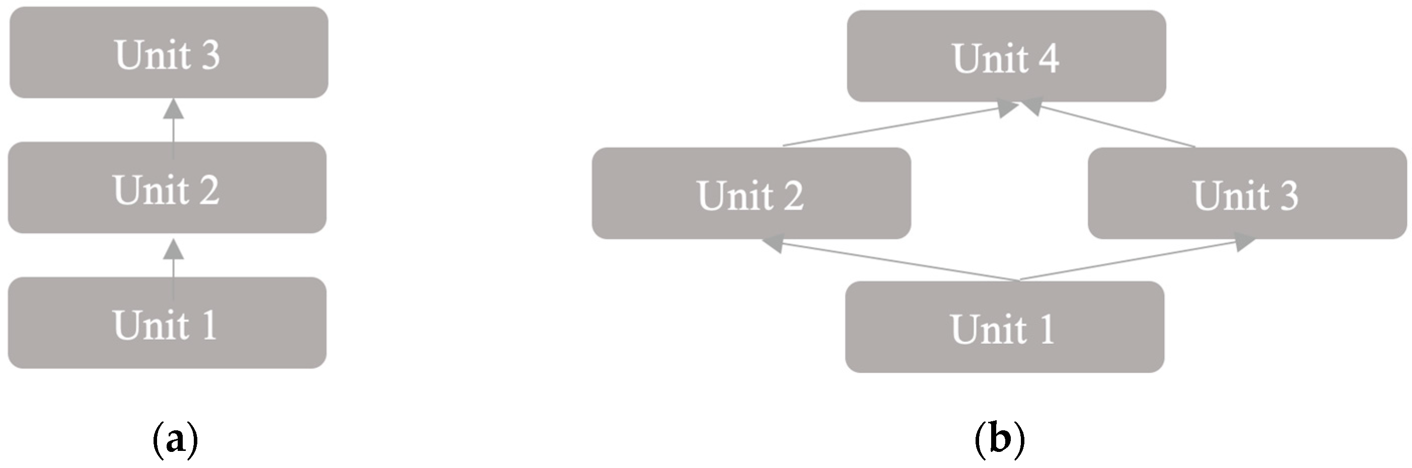
3] that moving from fully connected to sparsely connected architectures, even inside of the convolutions, gives a more accurate performance. This idea is based on Arora and his colleagues’ initial theoretical contribution, who stated that sparsity could be exploited by clustering correlated outputs [
15]. Sparse architecture involves increasing the network’s width instead of stacking connected layers. This approach contrasts with the fully connected architecture, where the layers are stacked on top of each other. The conceptual differences between the two architectures are illustrated in
Figure 1.
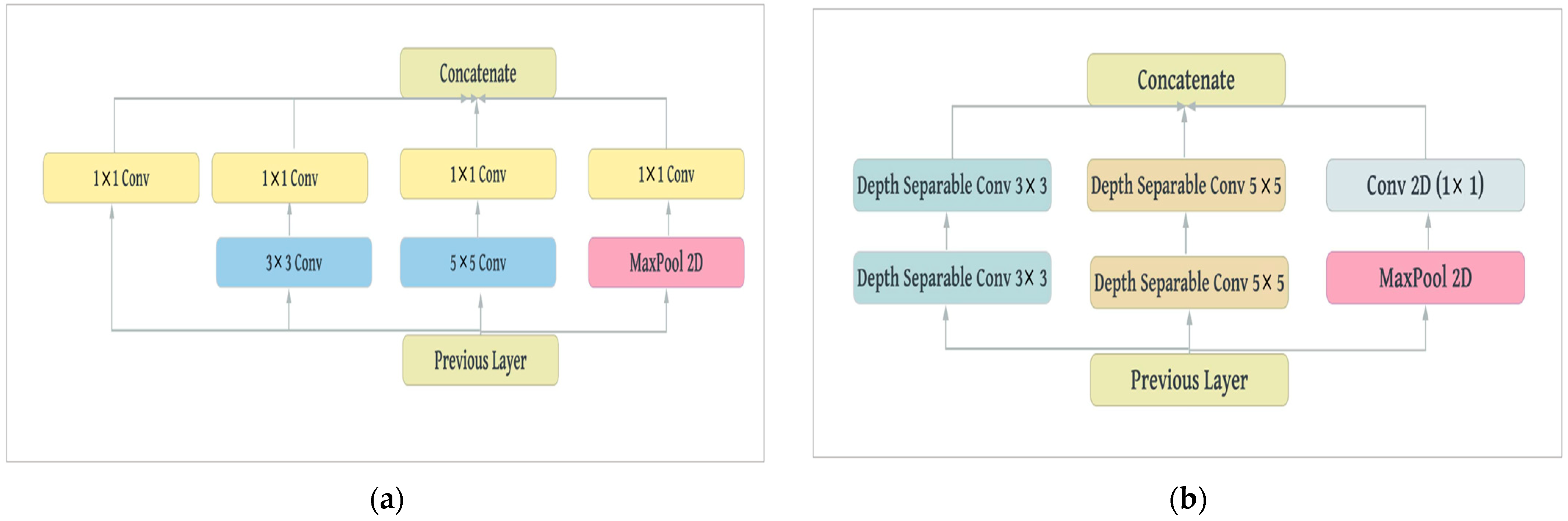
The next step is choosing the right filter sizes inside of these sparsely connected blocks. The salient parts in the images can significantly vary in size, and the area occupied by the object of interest can differ from one image to another. Due to this huge variation in object locations, choosing the appropriate filter size for the convolution operation becomes more challenging. A filter with a large dimension is preferred for information that occupies a larger space, while a smaller filter dimension is preferred for information that takes up a smaller space. Inception solves this issue by using different scale filters in one block in order to enable the internal layers to select the relevant scale to learn information. Inception uses 1 × 1, 3 × 3, and 5 × 5 filters and a parallel max-pooling layer, followed by 1 × 1 convolution, to reduce the complexity. These filters are useful for localization and object detection. To reduce the computational complexity of the Inception block, regular convolutions are replaced with depth-wise separable convolutions. We removed all of the 1 × 1 convolutional layers, except for the one, which was used after the max-pooling layer. Since depth-wise separable convolutions can learn features better than regular convolutions, we removed the parallel 1 × 1 convolutional layer. The proposed block consists of two stacked 3 × 3 and two stacked 5 × 5 depth-wise separable convolutions, as well as a parallel max-pooling layer.
Comparing the proposed block to the Inception block, the former has two additional spatial detection layers than the latter. Despite this greater capacity, it has around 1500 (16.5% less) fewer parameters than the Inception block. With respect to the Inception block, both point-wise and depth-wise operations are followed by a ReLU non-linearity; however, depth-wise separable convolutions are usually implemented without non-linearities between these operations. The absence of any non-linearity leads to faster convergence and a better final performance. The experiments showed that the proposed depth-wise separable block performed better than the Inception block in terms of speed and accuracy.
Figure 2 shows both the proposed block and the Inception block.
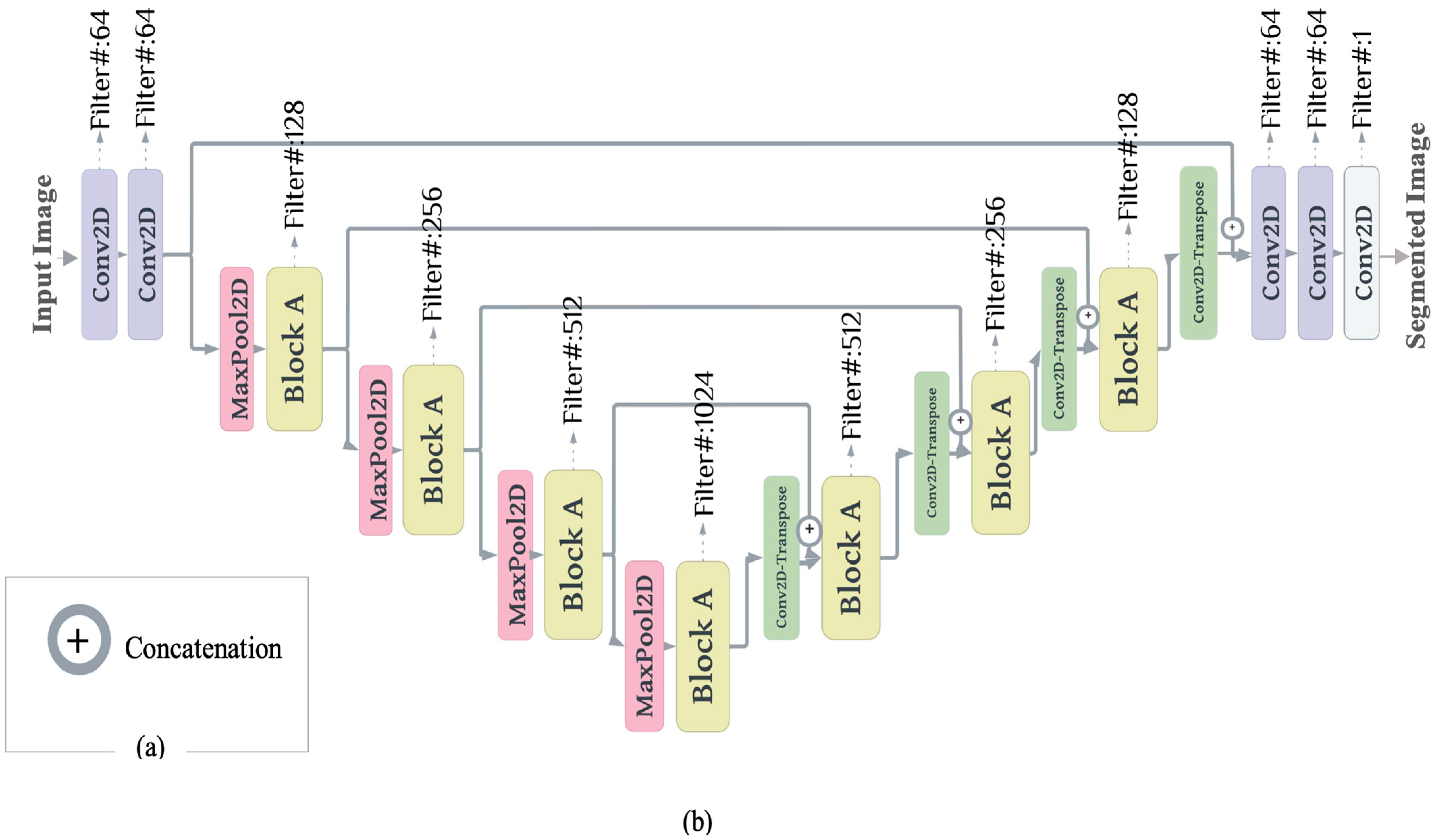
In general, the proposed depth-wise separable U-Net with multiscale filters starts with two 3 × 3 standard convolution blocks. It is suggested to avoid using depth-separable convolution in the initial layers; therefore, we used two standard convolutions instead, followed by three of the proposed blocks in the contracting path. Similar to U-Net, the output of each block acts as a skip connection for the corresponding decoder block. A max-pooling operation follows each block with stride two. The base layer contains one block, while the expansive path consists of three blocks, followed by two 3 × 3 standard convolutional layers. Each block in this path and the standard convolutional layers are preceded by a transposed convolutional layer. The final layer is a 1 × 1 convolution with sigmoid activation to generate the segmentation masks.
In sum, the proposed model consists of five standard convolutional layers and nine sparsely connected depth-wise separable blocks. We compare the proposed model’s performance with the original U-Net and three of its variants. For comparison purposes, we unified the number of filters in each layer for all of the models. The first layer starts with 64 filters and doubles after each max-pooling operation. The proposed block consists of multiple convolutional layers at each level; therefore, we divided the number of filters between each convolution in the internal block.
Figure 3 depicts the proposed model and the corresponding filter’s details.
3.2. Autoencoder Architecture
An autoencoder is an unsupervised artificial neural network that is capable of learning dense representations of the input data known as latent representations or coding. It consists of the following three parts: (a) the encoder network that acts as a feature detector; (b) the coding layer that saves the extracted features that typically have a much lower dimensionality than the input data; (c) and, finally, the decoder model that is used to reconstruct the original data. The autoencoder is useful for dimensionality reduction and visualization. It can further be used for pre-training a deep neural network, acting as a feature detector. The autoencoder can also randomly generate new data that appear similar to the training data, often known as the generative model [
16].
Annotating our sinkhole dataset for the semantic segmentation task was laborious and required expertise to identify the sinkholes. To automate the process, we built an autoencoder network and, in order to enable the autoencoder to reconstruct a binary mask image, binary cross-entropy loss was used. The reconstruction task was treated as a binary classification problem where each pixel’s intensity represents the probability that the pixel should be black or white.
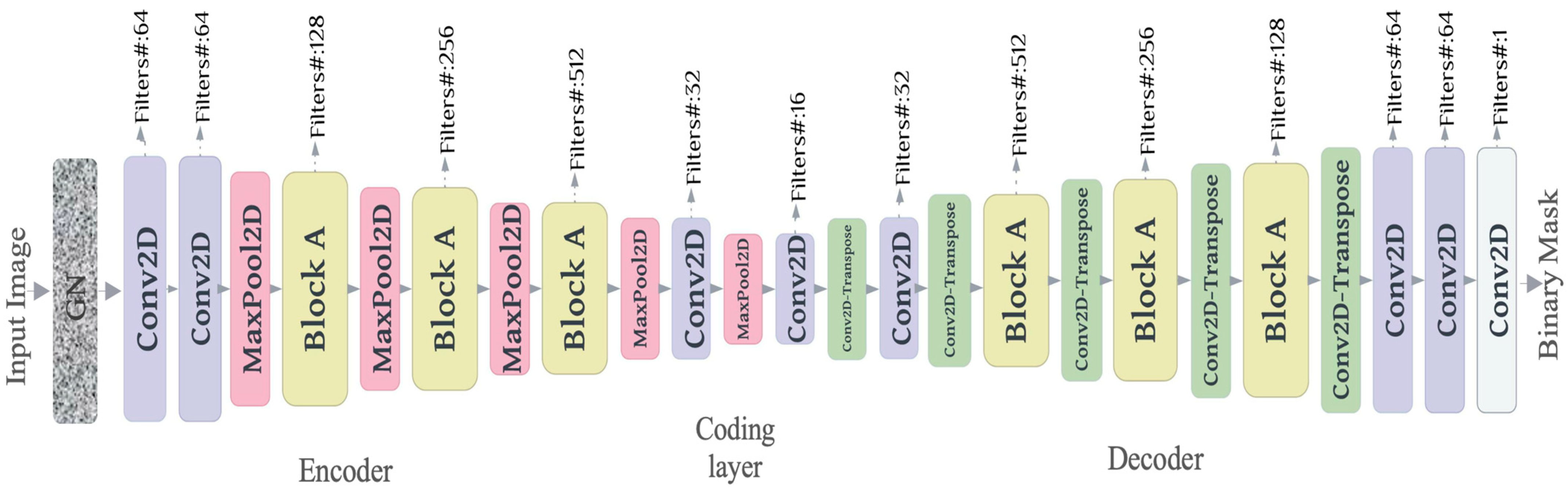
The decoder aims to reconstruct the original input as precisely as possible. It tries to copy the input; in this case, it may reconstruct a binary image that includes the sinkhole and all other background details. Two constraints are added to the network in order to force the autoencoder to focus, extract the sinkholes, and discard the other features. The first constraint is adding a GN layer—a natural choice of corruption method for real-valued inputs—after the autoencoder’s input layer. Adding noise to the autoencoder during training makes it learn useful features instead of copying and memorizing the input images. It is also useful to mitigate the overfitting problem, improving the network’s robustness.
The second constraint is limiting the size of the latent representations—the coding layer. The size of the latent representation is an important hyperparameter. When it is set to a small number, it forces the encoder to retain only the useful objects and discard any non-relevant or background features. The encoder consists of an input layer, followed by a GN layer, and three depth-wise separable blocks. A max-pooling layer for down-sampling follows each block. The decoder consists of the same encoder blocks, with each followed by a transposed convolution to reconstruct the input’s size. The autoencoder architecture is shown in
Figure 4.
3.3. Sinkhole Dataset Acquisition
The dataset is created by collecting 1001 positive and 303 negative samples of sinkhole images. The positive samples are simply images with sinkholes, whereas negative samples are composed of puddles, small ponds, potholes, and images without sinkholes. Sinkholes are surface deformations that involve either the collapse of the ground to form a depression or the slow subsidence of sediments near the surface, where water meets the land. They may form naturally or through human activities [
17] (for more information about sinkhole formation, see
Appendix A). A puddle is a small pool of water that forms on the ground after rainfall or near a water source. They are usually shallow and can be found on any flat surface. Ponds, on the other hand, are larger bodies of water that accumulate on the ground surface. They can be formed by rainfall, natural springs, or by human-made structures such as dams. Sometimes, ponds and puddles have features in common with sinkholes, such as depressions or a hole in the ground. Therefore, it is essential to carefully examine the characteristics and causes of a land depression before identifying it as a sinkhole. Potholes are minor ground deformations that are usually caused by degradation and wear and tear. They are usually formed on paved surfaces, such as roads, sidewalks, or parking lots, as a result of freeze–thaw cycles, heavy traffic, or poor construction quality. In terms of their physical appearance, both sinkholes and potholes can have similar characteristics, such as circular or irregular shapes and depth; however, sinkholes are generally much deeper and wider than potholes. Additionally, sinkholes can be caused by a variety of factors, such as natural geological processes or human activities, while potholes are mainly caused by natural weathering and erosion. The images without sinkholes, which comprise the fourth category in the negative samples, were created by removing the sinkholes from some of the positive images and keeping the background using Photoshop. This was carried out in order to ensure that the negative samples closely resembled the positive samples in terms of the surrounding background and terrain features while still being distinctly different from the positive samples in terms of the absence of sinkholes.
Having the model trained on negative samples as well as positive samples increases the success of the training. The negative image samples are chosen carefully in order to create a robust model that is capable of efficiently distinguishing between the sinkhole and non-sinkhole areas. Initially, we trained the model solely on positive samples, but when it was tested on negative samples, it failed to distinguish between sinkholes and non-sinkhole images. To address this, we collected the above-mentioned types of ground deformations and added them to the negative samples in order to teach the model their distinctive features and enable accurate discrimination.
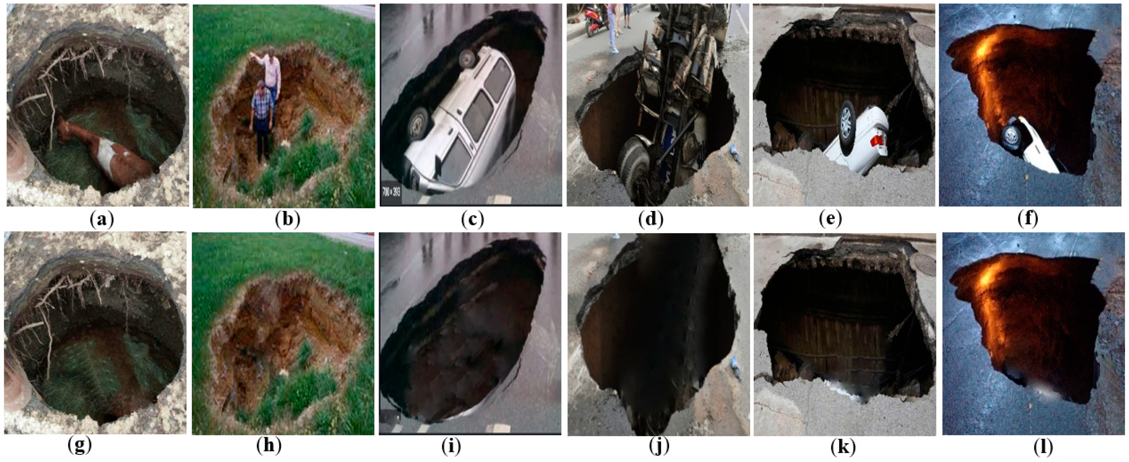
Sinkholes emerge suddenly in different areas; therefore, they may swallow the above surface objects. Most of the collected positive images contain objects such as vehicles, animals, traffic cones, and even humans inside sinkholes. We used Photoshop to remove these objects manually to enable the segmentation models to learn and extract sinkhole features rather than non-useful features for segmentation tasks. The presence of objects in the image could lead to the model learning features of those objects instead of the sinkholes, which would result in inaccurate or incomplete segmentation. Therefore, removing the objects helped to improve the accuracy and reliability of the model’s segmentation results. The images are resized into 256 × 256. Some samples are shown below in
Figure 5.
As previously stated, the dataset is quite large, and using it for supervised training requires annotation. Manual annotation can be a time-consuming process. Therefore, to address this challenge, we propose using an autoencoder that is capable of learning to reconstruct binary masks through the minimization of binary cross-entropy loss, as described in
Section 3.2. By utilizing this approach, we can automatically annotate the dataset.
3.4. Measuring the Model’s Reliability Using a Benchmark Cell Nuclei Segmentation Dataset
To further evaluate our model’s performance, in addition to the sinkhole dataset, we used the 2018 Data Science Bowl dataset for cell nuclei segmentation [
18]. The nuclei segmentation dataset contains around 700 segmented cell images in its first stage. The images were acquired under various conditions, cell types, magnifications, and imaging modalities. Biomedical image segmentation requires accurate image partitioning into multiple regions representing the anatomical objects of interest. It presents significant technical challenges, including shape, size, and texture variations, noisy boundaries, and/or a lack of consistency in source data acquisition. Therefore, the cell nuclei dataset was deemed to have a great degree of complexity, providing a suitable reliability test to gauge our model’s performance.
4. Implementation
This section discusses the data augmentation, optimization, and regularization methods that were applied to set the autoencoder and the segmentation models to training. By implementing these techniques, we aimed to improve the models’ ability to extract the relevant features from the images and prevent overfitting during the training process.
4.1. Data Augmentation
Data augmentation is a set of techniques used to artificially increase the amount of data by generating new samples from the existing ones. This is performed by applying some random transformations that yield plausible images, such as rotations, zooming, and flipping. The aim of the model was to never encounter the same image twice during training. This helps the model to gain exposure to additional aspects of the data and achieve better generalization [
4]. Data augmentation acts as a regularizer and helps to reduce the risk of overfitting [
19]. By applying data augmentation, we increased the diversity of the training data and reduced the chance of the model memorizing the training data, which can lead to a poor performance on new data. We used various augmentation techniques, including rotation, flipping, scaling, and shifting, which helped the model to learn invariance to these transformations and improved its performance on unaltered images. Three augmentation techniques were used on the positive dataset to train and improve the autoencoder annotation since the autoencoder was trained only on positive images. These techniques were rotation, horizontal flipping, and cropping of the original images. The size of the positive image dataset following augmentation was 2000 images.
Figure 6 shows an example of these techniques.
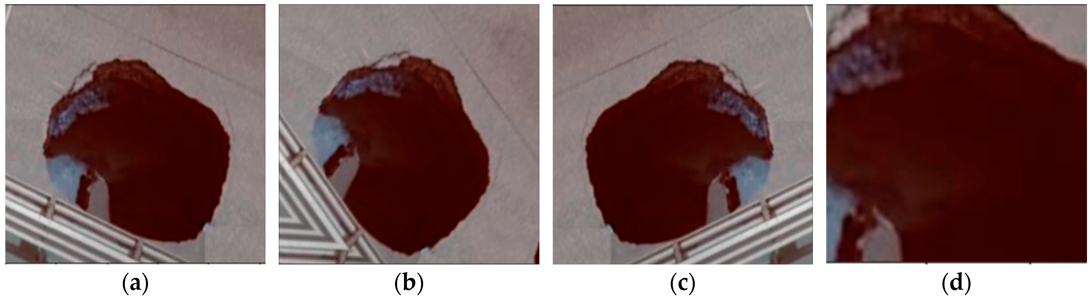
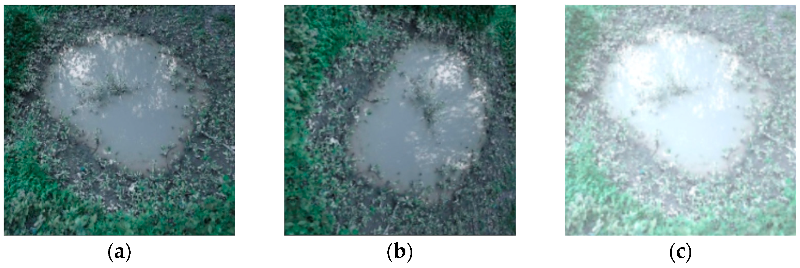
As mentioned earlier, the sinkhole dataset was imbalanced, with 1001 positive samples and only 303 negative samples. Training models on imbalanced data can cause them to be biased towards predicting the larger class and ignore the smaller class. To address this issue, we applied rotation and brightness augmentation techniques to the negative samples. These techniques resulted in the creation of 1001 new images, doubling the total number of images in the dataset to 2002. The augmented dataset was then used to train the segmentation models.
Augmenting the data not only balanced the dataset, but also introduced more variability and diversity, allowing the model to learn and generalize better.
Figure 7 illustrates an example of the augmentation techniques that were used on the negative samples, showing the original image and its rotated and brightened versions.
4.2. Optimization and Regularization
4.2.1. Dropout
In order to achieve a balance between model performance and overfitting, we included a dropout layer rate before the output layer in the segmentation models. We experimented with different dropout rates during the model training process and ultimately chose a rate of 0.1 for both of the dataset experiments. We selected this rate because it effectively prevented overfitting without compromising the model’s ability to accurately identify the sinkholes.
4.2.2. Optimization
For the autoencoder optimization, an Adam optimizer with a 0.001 learning rate was used. An Adam optimizer was also used to optimize the segmentation models on both of the datasets; the initial learning rate was set at 0.001, with an exponential learning rate decay of 10-4. The decay began after the first 20 epochs.
5. Results
This section discusses the autoencoder results and the proposed segmentation model’s results compared to U-Net and three other variants.
5.1. Autoencoder Annotation Results
Automated image annotation using an autoencoder model significantly reduced the time and effort required compared to manual annotation. As discussed in
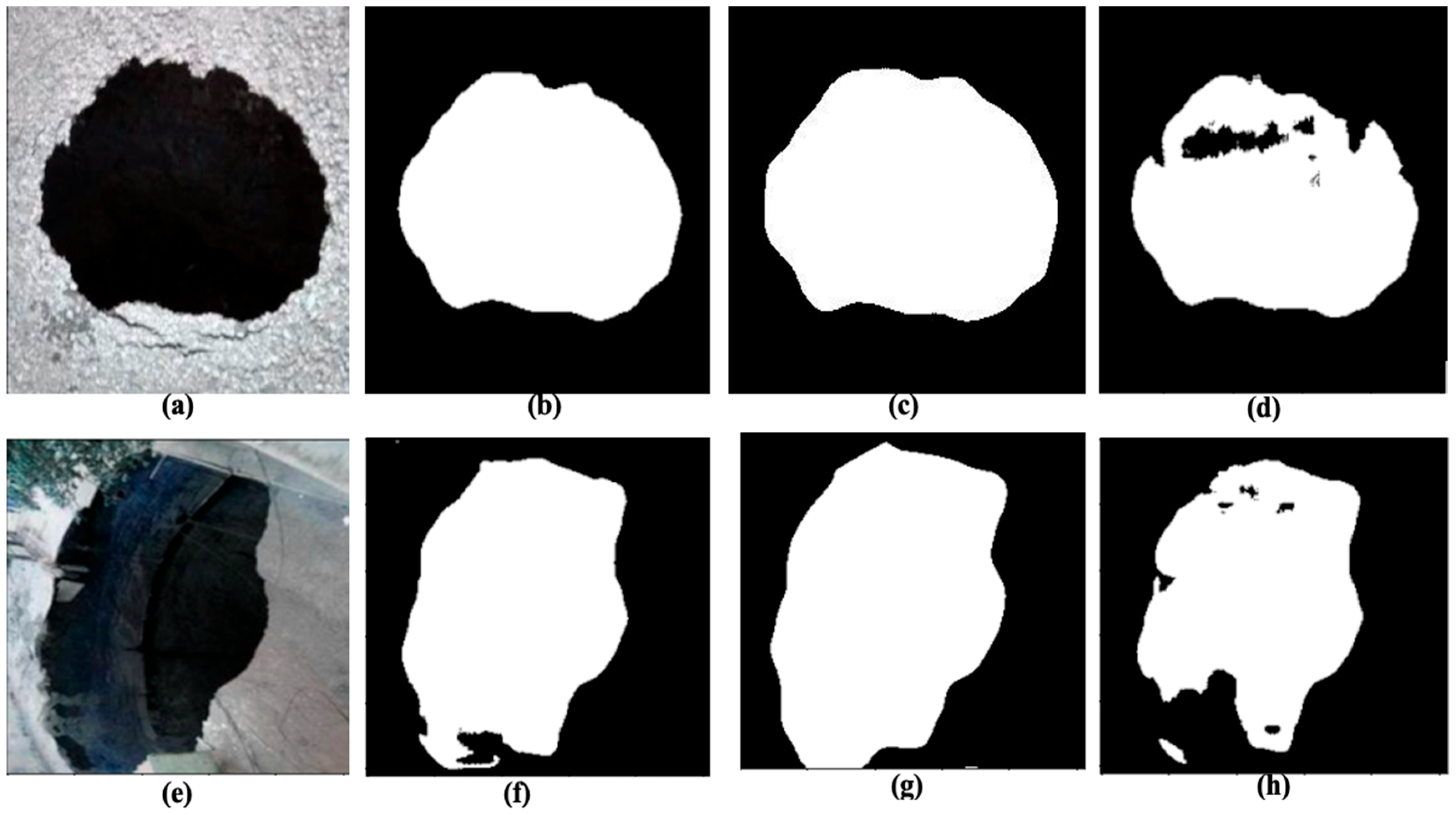
Section 3.2, the size of the autoencoder’s coding layer is an important hyperparameter. Therefore, an experiment with three different sizes was conducted to find the optimal size: 8 × 8, 4 × 4, and 16 × 16. The results of the autoencoder annotation with three different coding sizes are shown in
Figure 8.
5.2. The Proposed Model Results
Our model’s results have been compared to U-Net, Attention U-Net, Depth-Separable U-Net, and Inception U-Net. The latter is created by replacing the proposed block with the Inception block to study the effect of depth-separable convolution. The 1 × 1 layers of the Inception block are set to 40 filters to reduce the computation complexity. The number of filters in each convolution is unified in order to compare the models. The models start with 3 × 3 repeated convolutional blocks with 64 filters, doubling the number of filters after each max-pooling operation. The performance is evaluated in terms of IoU. The proposed model has a significantly smaller number of parameters than the other models. The proposed model’s parameters are approximately 5.1 M, which is 83%, 84%, 13%, and 76% less than U-Net, Attention U-Net, Depth-Separable U-Net, and Inception U-Net, respectively, as shown in
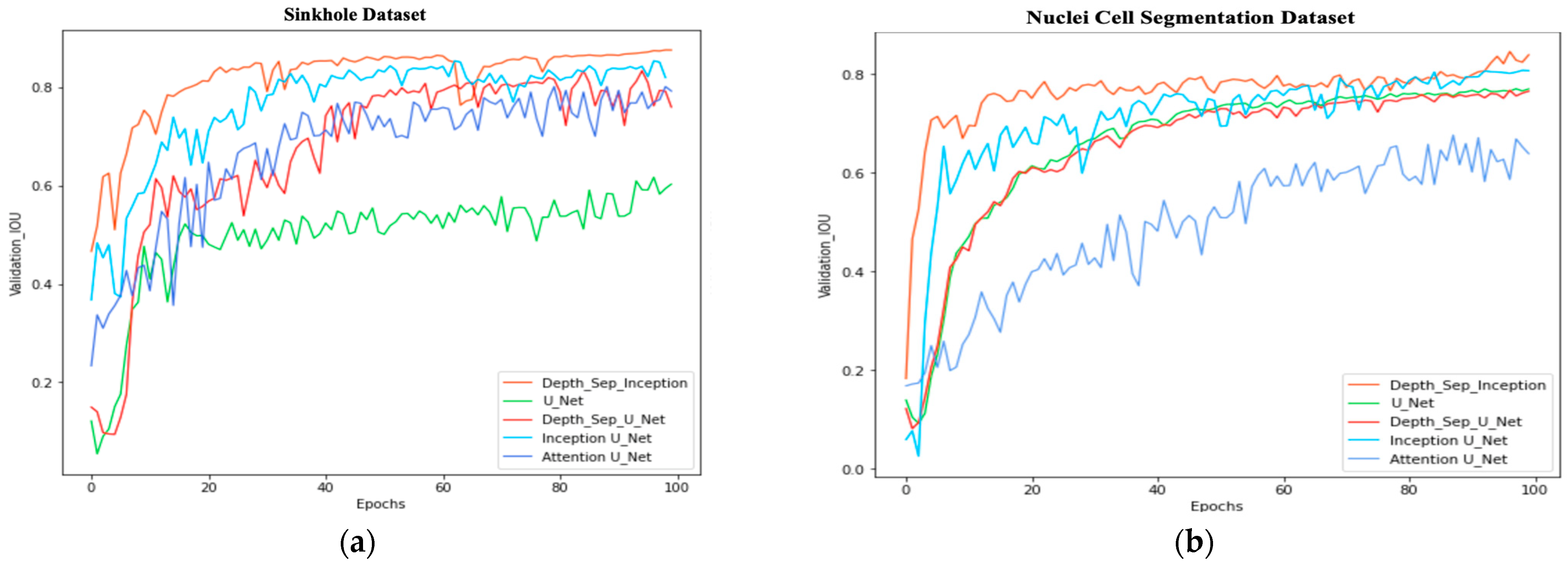
Table 1. The proposed model outperformed the other models on the two datasets; however, the Inception model’s results nearly paralleled our results. A validation graph is depicted in
Figure 9 for the sinkhole and nuclei segmentation datasets. The results are presented in
Table 2 and
Table 3, respectively.
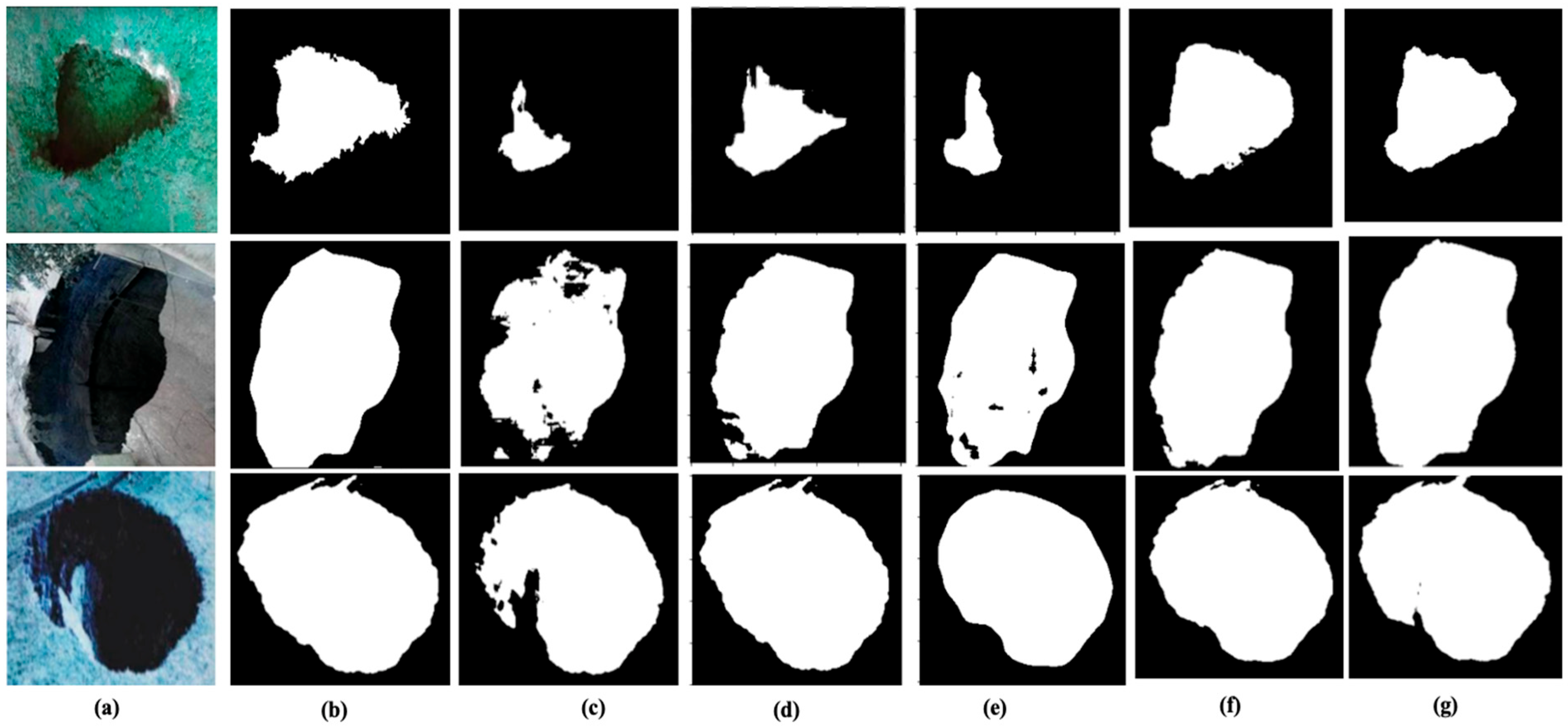
The experiments show that the proposed model can accurately localize and segment the objects.
Figure 10 compares the segmentation models on some of the samples from the sinkhole dataset. In the first row, the sinkhole has different lighting conditions. While U-Net, Attention U-Net, and Depth-Separable U-Net failed to segment the entire region, Inception U-Net and our model accurately segmented the region.
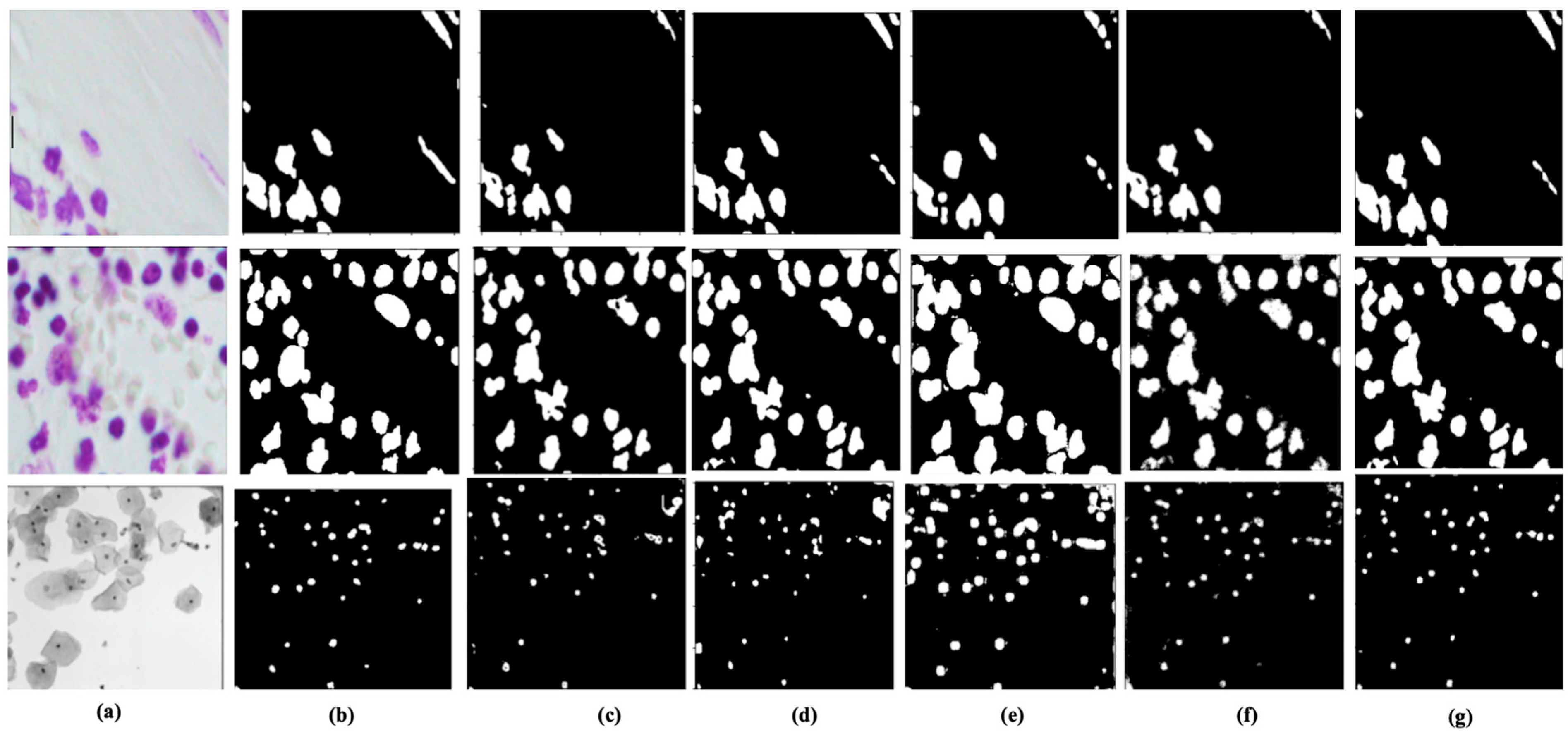
Figure 11 shows the model’s visual results on the biomedical nuclei segmentation datasets.
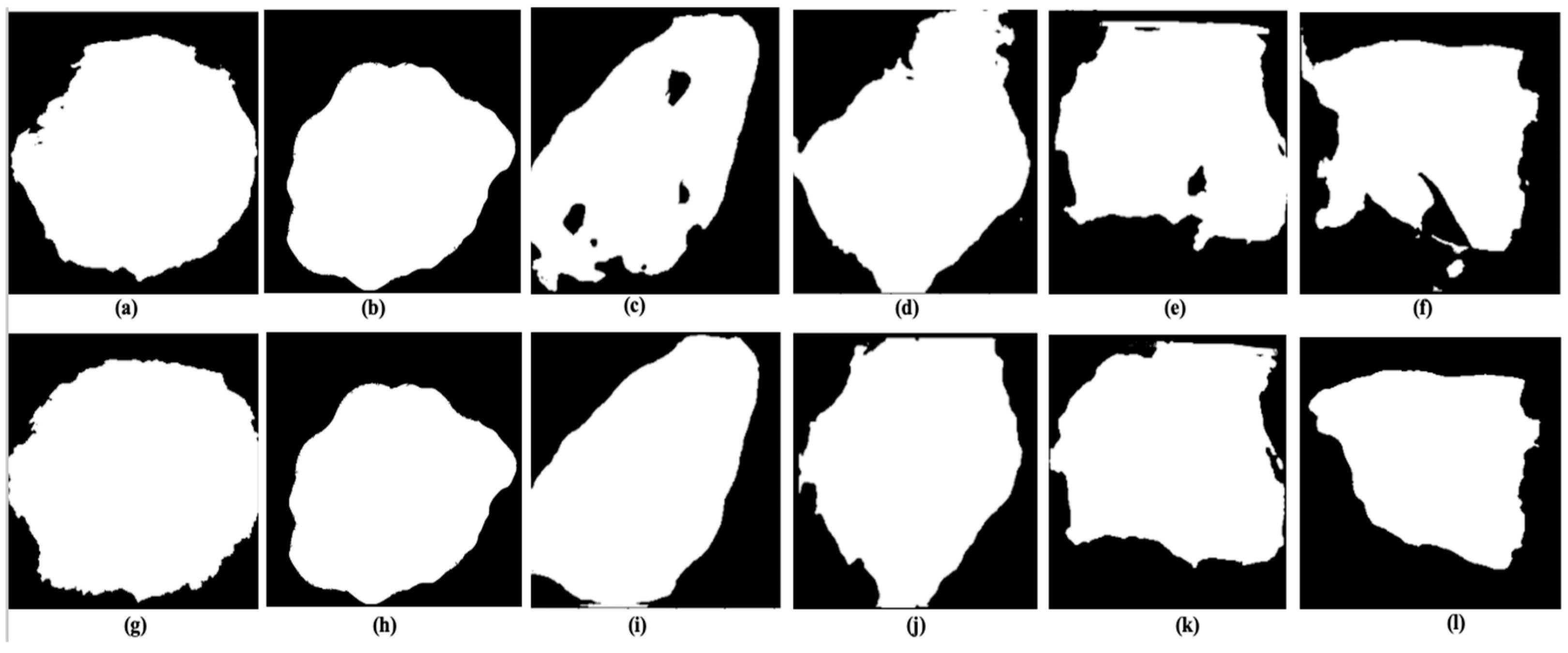
In order to optimize the performance of the sinkhole detection models, the sinkhole images were carefully curated using Photoshop to remove the non-sinkhole objects, as discussed in detail in
Section 3.3. However, in real-time inference, the images are usually not preprocessed in this way before being fed to the model. Therefore, it is important to evaluate the model’s performance on un-curated images, which more closely resemble the type of input that the model would receive in a real-world scenario.
The experiments that were conducted in this study demonstrate that the sinkhole detection model is capable of accurately segmenting and identifying sinkholes even when they are presented through un-curated images. The results of these experiments are presented in
Figure 12.
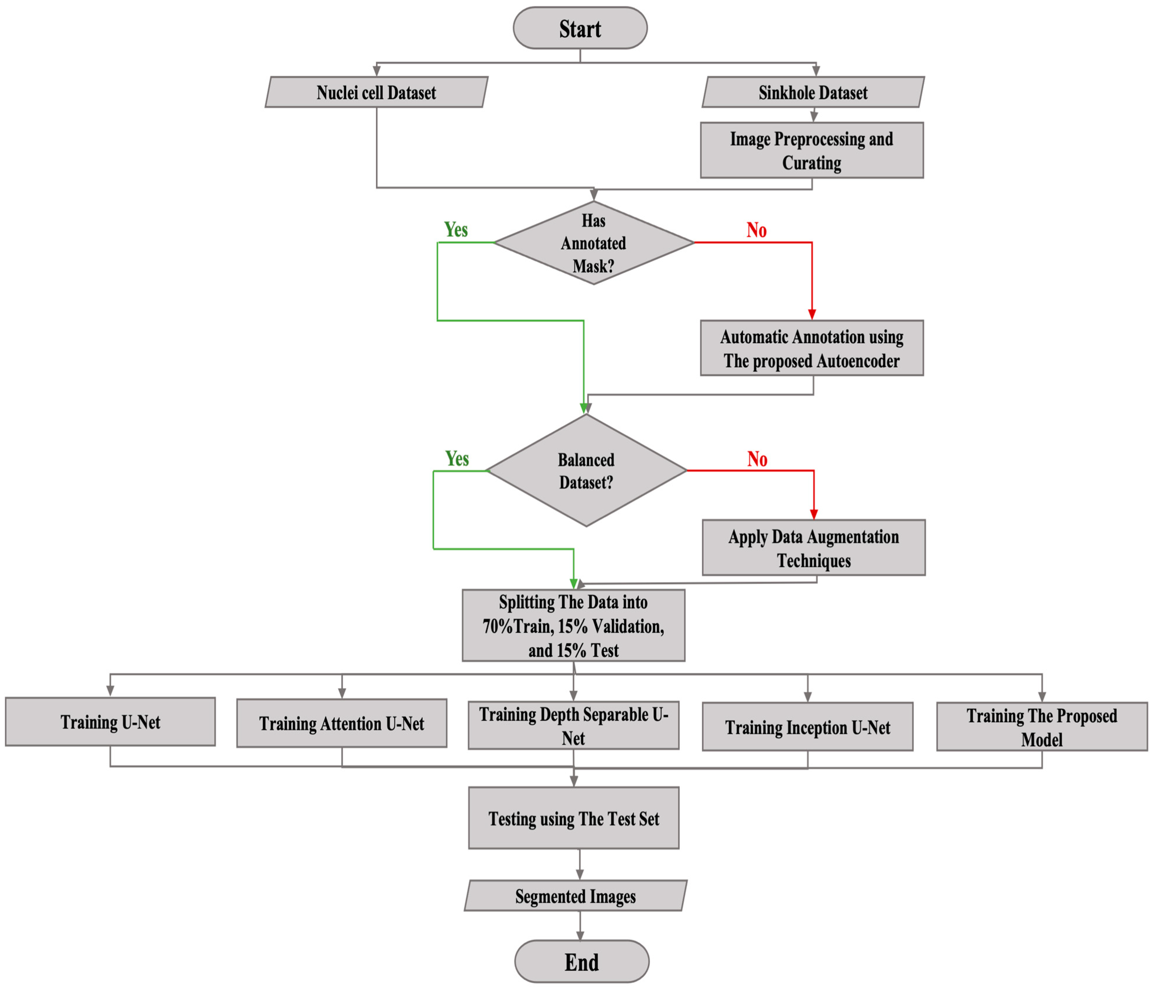
For a better understanding of the workflow that is involved in the model’s operation, we have provided a detailed workflow diagram in
Figure 13. This diagram illustrates the different stages that are involved in the sinkhole detection process, from image acquisition and preprocessing to final sinkhole detection and segmentation. Overall, our experiments show that our sinkhole detection model is effective and can be applied in real-world scenarios without the need for extensive preprocessing of images.
6. Discussion
We demonstrate that the proposed autoencoder is an effective and efficient method for automated image annotation, showcasing the potential of deep learning techniques in significantly reducing the time and effort required compared to manual annotation. The conducted experiment involved testing the autoencoder model with three different sizes of coding layers to identify the optimal size, which was determined to be 8 × 8, as shown in
Figure 8. The results showed that an 8 × 8 size yielded better quality annotated images. The autoencoder annotation results were verified manually. Most of the images were accurately annotated, except for nearly 60 images. These images reconstructed the sinkhole alongside some background noise. The noise was removed manually.
The proposed segmentation model’s performance was compared to U-Net, Attention U-Net, Depth-Separable U-Net, and Inception U-Net, and it outperformed the other models on both of the datasets with a higher validation IoU than the other models. However, the Inception model’s results were comparable to the proposed model’s, given that we designed it to be similar to our proposed model in order to investigate the effect of standard convolutions compared to depth-wise separable convolutions.
The visual results show that the proposed model has the highest quality predicted binary mask and can accurately detect and segment the required objects, even under varying lighting conditions, as shown in
Figure 10. Therefore, we suggest using it for biomedical image segmentation, where the accuracy of the predicted regions is crucial.
Additionally, the proposed model has significantly fewer parameters than the other models, as shown in
Table 2, resulting in faster training and less space consumption.
Our experiments have demonstrated that the proposed model is robust and capable of identifying and segmenting sinkholes, even with real-world un-curated images, as illustrated in
Figure 12.
7. Conclusions
In sum, this paper proposes a deep learning model for semantic segmentation tasks, which is an improved version of U-Net that uses a sparsely connected block with multiscale filters to achieve a greater performance with a reduced capacity. To evaluate our model, a sinkhole dataset was manually collected from different sources, curated, and automatically annotated using the proposed autoencoder that reduced the annotation time while producing accurate masks. A benchmark nuclei dataset was then used to further evaluate the model’s performance and reliability.
The proposed model can be extended to other deep learning areas, including challenging biomedical imaging segmentation tasks. The main advantage of our model is a significant gain in quality without the increased computational resources. In comparison to U-Net, Attention U-Net, Depth-Separable U-Net, and Inception U-Net, our model performed better on both the sinkhole and the nuclei segmentation datasets, achieving an average improvement of 1.2% and 1.4%, respectively, with a 94% and 92% accuracy, respectively. Furthermore, our model achieved 83% and 80% IoU on the two datasets—an average improvement of 11.8% and 9.3% over the above-mentioned models, respectively.
Experimentally, it was found that the depth-wise separable convolution learns better features when compared to the standard convolution. This conclusion is based on two experiments. The first was conducted by comparing the U-Net visual and numerical results with the depth-wise separable U-Net, with both having the same architecture. The only difference was the use of depth-wise separable convolution in the latter model. The second experiment was conducted by comparing the proposed model with the Inception model, which also had a similar architecture. The Inception model was built by replacing the proposed block with the Inception block, which differed from the former in the use of standard convolutions, in addition to having two additional 1 × 1 convolutional layers after the 3 × 3 and the 5 × 5 layers in order to reduce the computational complexity. The results showed that the use of depth-wise separable convolutions is effective enough to improve the IoU score, in addition to the advantage of reducing the network’s complexity.
The experiments also showed the robustness of the proposed model in predicting un-curated images, as well as images with different objects inside the sinkholes, which makes the model efficient in predicting real-time images, such as those that are used by drone systems, without the need for additional preprocessing steps.
This is a significant finding because it suggests that the proposed model could be used in practical applications, such as drone-based surveillance systems for sinkhole detection and monitoring. These systems could play a crucial role in mitigating the risk of harm and economic losses that are caused by sinkholes by enabling early detection and prompting action.
The fact that the model can predict sinkholes from un-curated images and images with different objects inside sinkholes means that it could be used in a wide range of scenarios without requiring significant manual intervention or additional preprocessing. Overall, the experiments have provided strong evidence for the effectiveness and practicality of the proposed model.
Author Contributions
Conceptualization, R.A. and M.T.H.; methodology, R.A.; software, R.A.; validation, R.A., M.C.F. and M.T.H.; formal analysis, R.A. and M.T.H.; investigation, R.A.; resources, M.C.F. and M.T.H.; data curation, R.A.; writing—original draft preparation, R.A. and M.T.H.; writing—review and editing, R.A., M.T.H., M.C.F.; visualization, R.A.; supervision, M.T.H.; project administration, M.T.H.; funding acquisition, M.T.H. All authors have read and agreed to the published version of the manuscript.
Funding
This research received no external funding.
Informed Consent Statement
Not applicable.
Data Availability Statement
Acknowledgments
We gratefully acknowledge Mostafa Mashhad for reviewing this paper. We are also thankful to Murtada Mousa, P.E., for his expertise and thorough assessment of the reliability of the sinkhole dataset.
Conflicts of Interest
The authors declare no conflict of interest.
Appendix A. Sinkholes Formation
Sinkholes, also known as dolines [
20], are common in karst geographical terrains. Karst is associated with soluble rocks, such as limestone, dolomite, and other carbonate rocks, which can create sinkholes by dissolving the bedrock. Besides solution sinkholes, there could also be cover–subsidence sinkholes or cover–collapse sinkholes. Sinkholes may also form naturally or through human activities [
17]. Natural sinkholes form from underground water flow, levee seepage, or excess rainwater infiltrating the soil. Human-induced sinkholes result from human activities such as unsealed sewers or water leakages in underground pipelines and drainage systems [
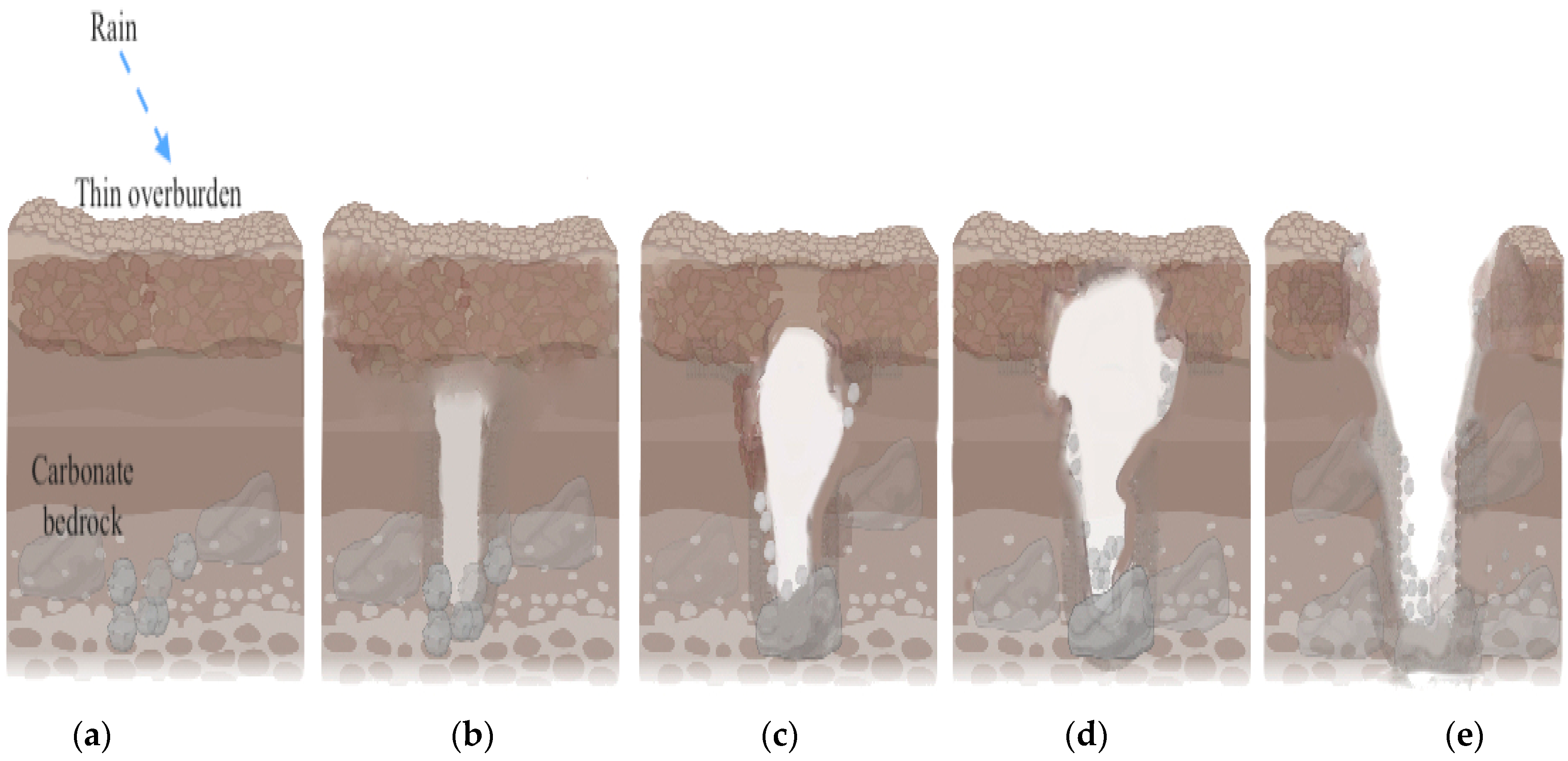
21]. When water percolates through the soil, the underground bedrocks absorb the water and begin to erode, forming underground spaces and cavities. The erosion of the carbonate bedrock will develop upward through the overlying sediments toward the land surface. When there is insufficient support from the underlying ground, the surface eventually collapses, creating sudden and catastrophic sinkholes. The formation process is depicted in
Figure A1 [
17].
Figure A1.
The gradual formation of a sinkhole from rainwater: (
a) water gathers in thin overburden; (
b–
d) the water percolates through the soil, causing erosion and dissolution of carbonate bedrocks overtime; and (
e) surface collapse forming sinkhole [
17].
Figure A1.
The gradual formation of a sinkhole from rainwater: (
a) water gathers in thin overburden; (
b–
d) the water percolates through the soil, causing erosion and dissolution of carbonate bedrocks overtime; and (
e) surface collapse forming sinkhole [
17].
The United States Geological Survey (USGS) reports that approximately 20% of land in the US is at risk of sinkholes [
22]. Studies have found that many of these sinkholes are caused by human activities, such as drilling, mining, construction, and broken drainpipes [
20]. One particularly notable example occurred on 3 August 2012, in Bayou Corne, Louisiana, where a massive sinkhole was accidentally created while drilling for concentrated salt. The collapse resulted in the release of oil and methane gas from underground, which appeared as visible bubbles on the surface of the water. The sinkhole initially covered an area of 2.5 acres, but, by 2014, it had expanded to cover 26 acres [
23]. The area was evacuated, and some residents were unable to return [
24].
The economic damages that are caused by sinkholes have been estimated to be at least USD 300 million per year. However, because there is no national tracking system for sinkhole damage costs, this estimate is likely to be much lower than the actual damage cost [
25]. As a result, it is crucial to develop methods for detecting and monitoring sinkholes in order to mitigate the risk of harm and economic losses.
References
- Bali, A.; Singh, S.N. A Review on the Strategies and Techniques of Image Segmentation. In Proceedings of the Fifth International Conference on Advanced Computing & Communication Technologies, Haryana, India, 21–22 February 2015; pp. 113–120. [Google Scholar]
- Ronneberger, O.; Fischer, P.; Brox, T. U-net: Convolutional Networks for Biomedical Image Segmentation. In Proceedings of the International Conference on Medical Image Computing and Computer-Assisted Intervention, Munich, Germany, 5–9 October 2015; Springer: Cham, Switzerland; pp. 234–241. [Google Scholar]
- Szegedy, C.; Liu, W.; Jia, Y.; Sermanet, P.; Reed, S.; Anguelov, D.; Erhan, D.; Vanhoucke, V.; Rabinovich, A. Going Deeper with Convolutions. In Proceedings of the IEEE Conference on Computer Vision and Pattern Recognition, Boston, MA, USA, 7–12 June 2015; pp. 1–9. [Google Scholar]
- Chollet, F. Deep Learning with Python, 1st ed.; Manning Publications: New York, NY, USA, 2018. [Google Scholar]
- Oktay, O.; Schlemper, J.; Folgoc, L.L.; Lee, M.; Heinrich, M.; Misawa, K.; Mori, K.; McDonagh, S.; Hammerla, N.Y.; Kainz, B.; et al. Attention u-net: Learning where to look for the pancreas. arXiv 2018, arXiv:1804.03999. [Google Scholar]
- Liu, R.; Jiang, D.; Zhang, L.; Zhang, Z. Deep depthwise separable convolutional network for change detection in optical aerial images. IEEE J. Sel. Top. Appl. Earth Obs. Remote Sens. 2020, 13, 1109–1118. [Google Scholar] [CrossRef]
- Vanhoucke, V. Learning visual representations at scale. ICLR Invit. Talk 2014, 1. [Google Scholar]
- Panta, M.; Hoque, M.; Abdelguerfi, M.; Flanagin, M.C. IterLUNet: Deep Learning Architecture for Pixel-Wise Crack Detection in Levee Systems. IEEE Access 2023, 20, 6. [Google Scholar] [CrossRef]
- Panta, M.; Hoque, M.; Abdelguerfi, M.; Flanagin, M.C. Pixel-Level Crack Detection in Levee Systems: A Comparative Study. In Proceedings of the IGARSS 2022-2022 IEEE International Geoscience and Remote Sensing Symposium, Kuala Lumpur, Malaysia, 17–22 July 2022; pp. 3059–3062. [Google Scholar]
- Kuchi, A.; Hoque, M.; Abdelguerfi, M.; Flanagin, M.C. Machine learning applications in detecting sand boils from images. Array 2019, 3, 100012. [Google Scholar] [CrossRef]
- Chen, C.; Liang, J.; Xie, F.; Hu, Z.; Sun, W.; Yang, G.; Yu, J.; Chen, L.; Wang, L.; Wang, L.; et al. Temporal and spatial variation of coastline using remote sensing images for Zhoushan archipelago, China. Int. J. Appl. Earth Obs. Geoinf. 2022, 107, 102711. [Google Scholar] [CrossRef]
- Yang, G.; Huang, K.; Sun, W.; Meng, X.; Mao, D.; Ge, Y. Enhanced mangrove vegetation index based on hyperspectral images for mapping mangrove. ISPRS J. Photogramm. Remote Sens. 2022, 189, 236–254. [Google Scholar] [CrossRef]
- Sun, W.; Ren, K.; Meng, X.; Yang, G.; Xiao, C.; Peng, J.; Huang, J. MLR-DBPFN: A multi-scale low rank deep back projection fusion network for anti-noise hyperspectral and multispectral image fusion. IEEE Trans. Geosci. Remote Sens. 2022, 60, 1–14. [Google Scholar] [CrossRef]
- Al-Kouri, O.; Al-Rawashdeh, S.; Sadoun, B.; Sadoun, B.; Pradhan, B. Geospatial modeling for sinkholes hazard map based on GIS & RS data. J. Geogr. Inf. Syst. 2013, 5, 41238. [Google Scholar]
- Arora, S.; Bhaskara, A.; Ge, R.; Ma, T. Provable Bounds for Learning Some Deep Representations. In Proceedings of the International Conference on Machine Learning, Beijing, China, 21–26 June 2014; International Machine Learning Society (IMLS): Bellevue, WA, USA; pp. 584–592. [Google Scholar]
- Géron, A. Hands-on Machine Learning with Scikit-Learn, Keras, and TensorFlow: Concepts, Tools, and Techniques to Build Intelligent Systems; O’Reilly Media, Inc.: Sebastopol, CA, USA, 2019. [Google Scholar]
- Tihansky, A.B. Sinkholes, West-Central Florida; USGS: Reston, VA, USA, 1999; Volume 1182, pp. 121–140. [Google Scholar]
- Caicedo, J.C.; Goodman, A.; Karhohs, K.W.; Cimini, B.A.; Ackerman, J.; Haghighi, M.; Heng, C.; Becker, T.; Doan, M.; McQuin, C.; et al. Nucleus segmentation across imaging experiments: The 2018 Data Science Bowl. Nat. Methods 2019, 16, 1247–1253. [Google Scholar] [CrossRef] [PubMed] [Green Version]
- Shanthamallu, U.S.; Spanias, A.; Tepedelenlioglu, C.; Stanley, M. A Brief Survey of Machine Learning Methods and Their Sensor and IoT Applications. In Proceedings of the 2017 8th International Conference on Information, Intelligence, Systems & Applications (IISA), Larnaca, Cyprus, 27–30 August 2017; pp. 1–8. [Google Scholar]
- Gutiérrez, F.; Cooper, A. Surface Morphology of Gypsum Karst. Treatise Geomorphol. 2013, 6, 425–437. [Google Scholar]
- Ali, H.; Choi, J. A review of underground pipeline leakage and sinkhole monitoring methods based on wireless sensor networking. Sustainability 2019, 11, 4007. [Google Scholar] [CrossRef] [Green Version]
- Water Science School, Sinkholes, USA. Geological Survey, Scientific Agency. 2018. Available online: https://www.usgs.gov/special-topics/water-science-school/science/sinkholes#overview (accessed on 9 August 2022).
- Stanley, C. Bayou Corne Sinkhole: An Update on the Louisiana Environmental Disaster. Jonathan Turley. 2014. Available online: https://jonathanturley.org/2014/01/11/bayou-corne-sinkhole-an-update-on-the-louisiana-enviornmental-disaster/ (accessed on 9 August 2022).
- Jones, C.; Blom, R. Measurement of Sinkhole Formation and Progression with InSAR. In AGU Fall Meeting Abstracts; American Geophysical Union: Washington, DC, USA, 2013. [Google Scholar]
- USGS. Water Science School, Sinkhole Damages, USA. Geological Survey, Scientific Agency. Available online: https://www.usgs.gov/faqs/how-much-does-sinkhole-damage-cost-each-year-united-states#:~:text=Frequently%20Asked%20Questions-,How%20much%20does%20sinkhole%20damage%20cost%20each%20year%20in%20the,lower%20than%20the%20actual%20cost (accessed on 9 August 2022).
Figure 1.
The difference between fully (a) and sparsely (b) connected architectures.
Figure 1.
The difference between fully (a) and sparsely (b) connected architectures.
Figure 2.
(a) Inception block; and (b) Block A is the proposed depth-separable block. The proposed block has more spatial detector layers (3 × 3 and 5 × 5) with fewer trainable parameters.
Figure 2.
(a) Inception block; and (b) Block A is the proposed depth-separable block. The proposed block has more spatial detector layers (3 × 3 and 5 × 5) with fewer trainable parameters.
Figure 3.
The proposed multiscale depth-wise separable U-Net. Block A is the proposed depth-separable block shown in
Figure 2: (
a) concatenation operation; and (
b) the proposed multiscale depth-wise separable U-Net. The input image is progressively filtered and down-sampled by a factor of 2 at each layer in the contracting path on the left. The expansive path on the right performs up-sampling operations to reconstruct a binary-masked image. The number of filters at each layer is denoted on top of the block.
Figure 4.
The autoencoder’s architecture is used to annotate the sinkhole dataset. The input image is passed through a GN layer, progressively filtered, and down-sampled at each layer in the encoder part. The decoder path on the right performs up-sampling operations to reconstruct a binary-masked image. Block A is the separable depth block shown in
Figure 2. The coding layer size is 8 × 8, with 16 filters.
Figure 5.
The first row (a–f) shows the collected raw sample images, while the second row (g–l) shows the corresponding preprocessed and curated sample images. The corresponding curated image of the raw sample (a) is given in the sample column (g).
Figure 5.
The first row (a–f) shows the collected raw sample images, while the second row (g–l) shows the corresponding preprocessed and curated sample images. The corresponding curated image of the raw sample (a) is given in the sample column (g).
Figure 6.
Applying data augmentation techniques to increase training data while training the autoencoder: (a) is the original image; (b) random rotation; (c) horizontal flipping; and (d) random cropping.
Figure 6.
Applying data augmentation techniques to increase training data while training the autoencoder: (a) is the original image; (b) random rotation; (c) horizontal flipping; and (d) random cropping.
Figure 7.
Applying data augmentation techniques to increase the negative samples to balance the sinkhole dataset while training the segmentation models. (a) The original image; (b) random rotation; and (c) adjusted brightness. The figure shows a small puddle drawn from the negative samples.
Figure 7.
Applying data augmentation techniques to increase the negative samples to balance the sinkhole dataset while training the segmentation models. (a) The original image; (b) random rotation; and (c) adjusted brightness. The figure shows a small puddle drawn from the negative samples.
Figure 8.
Two examples of the autoencoder annotation results using three different coding layer sizes: (a) on the first row is the original image of the first sample; and (b–d) are the results of the autoencoder with a coding layer of size 4 × 4, 8 × 8, and 16 × 16, respectively. (e) On the second row is the original image of the second sample; and samples (f–h) are the results of the autoencoder with a coding layer of size 4 × 4, 8 × 8, and 16 × 16, respectively.
Figure 9.
Validation graphs of the segmentation models: (a) the IoU validation graph of the sinkhole dataset graph; and (b) the IoU validation graph of the Data Science Bowl dataset for nuclei cell segmentation. The proposed, depth-wise separable U-Net in the orange color shows the highest validation IoU compared to the other models.
Figure 10.
Visual comparisons among the segmentation models on the sinkhole dataset: (a) the original images; (b) the ground truth; (c) U-Net; (d) Depth-Separable U-Net; (e) Attention U-Net; (f) Inception U-Net; and (g) our model’s results.
Figure 10.
Visual comparisons among the segmentation models on the sinkhole dataset: (a) the original images; (b) the ground truth; (c) U-Net; (d) Depth-Separable U-Net; (e) Attention U-Net; (f) Inception U-Net; and (g) our model’s results.
Figure 11.
Visual comparisons among the segmentation models on the nuclei cell segmentation dataset: (a) the original images; (b) the ground truth; (c) U-Net; (d) Depth-Separable U-Net; (e) Attention U-Net; (f) Inception U-Net; and (g) the proposed model results.
Figure 11.
Visual comparisons among the segmentation models on the nuclei cell segmentation dataset: (a) the original images; (b) the ground truth; (c) U-Net; (d) Depth-Separable U-Net; (e) Attention U-Net; (f) Inception U-Net; and (g) the proposed model results.
Figure 12.
The robustness of the proposed model in predicting the un-curated images. The first row (
a–
f) shows the predicted masks of un-curated images from
Figure 5a–f, and the second row (
g–
l) shows the related predicted masks of curated images from
Figure 5g–l.
Figure 12.
The robustness of the proposed model in predicting the un-curated images. The first row (
a–
f) shows the predicted masks of un-curated images from
Figure 5a–f, and the second row (
g–
l) shows the related predicted masks of curated images from
Figure 5g–l.
Figure 13.
The workflow diagram. After preprocessing and curating the images, the next step is automatically annotating the dataset using the proposed autoencoder, balancing the dataset using data augmentation techniques, and training and evaluating the segmentation models, including the proposed model, using the training and validation sets. The final step is testing the models using the test set.
Table 1.
Comparisons of the Number of Trainable Parameters for the Segmentation Models.
Table 1.
Comparisons of the Number of Trainable Parameters for the Segmentation Models.
| Model | Trainable Parameters |
|---|
| U-Net | 31,031,745 |
| Attention U-Net | 32,430,151 |
| Depth-Separable U-Net | 5,983,873 |
| Inception U-Net | 21,635,897 |
| The proposed model | 5,185,817 |
Table 2.
Performance Evaluations of the Segmentation Models on the Sinkhole Dataset.
Table 2.
Performance Evaluations of the Segmentation Models on the Sinkhole Dataset.
| Model | IoU | Accuracy | Loss |
|---|
| U-Net | 0.7004 | 0.9132 | 0.2012 |
| Attention U-Net | 0.7256 | 0.9201 | 0.1968 |
| Depth-Separable U-Net | 0.7514 | 0.9392 | 0.1513 |
| Inception U-Net | 0.8038 | 0.9316 | 0.1288 |
| The proposed model | 0.8317 | 0.9446 | 0.1215 |
Table 3.
Performance Evaluations of the Segmentation Models on the Nuclei Cell Segmentation Dataset.
Table 3.
Performance Evaluations of the Segmentation Models on the Nuclei Cell Segmentation Dataset.
| Model | IoU | Accuracy | Loss |
|---|
| U-Net | 0.7435 | 0.9214 | 0.0703 |
| Attention U-Net | 0.6745 | 0.9034 | 0.1268 |
| Depth-Separable U-Net | 0.7616 | 0.9172 | 0.0659 |
| Inception U-Net | 0.7805 | 0.9139 | 0.1112 |
| The proposed model | 0.8067 | 0.9273 | 0.0554 |
| Disclaimer/Publisher’s Note: The statements, opinions and data contained in all publications are solely those of the individual author(s) and contributor(s) and not of MDPI and/or the editor(s). MDPI and/or the editor(s) disclaim responsibility for any injury to people or property resulting from any ideas, methods, instructions or products referred to in the content. |
© 2023 by the authors. Licensee MDPI, Basel, Switzerland. This article is an open access article distributed under the terms and conditions of the Creative Commons Attribution (CC BY) license (https://creativecommons.org/licenses/by/4.0/).


