
Characterizing Uncertainty and Enhancing Utility in Remotely Sensed Land Cover Using Error Matrices Localized in Canonical Correspondence Analysis Ordination Space
 , ,
, ,
Abstract
:1. Introduction
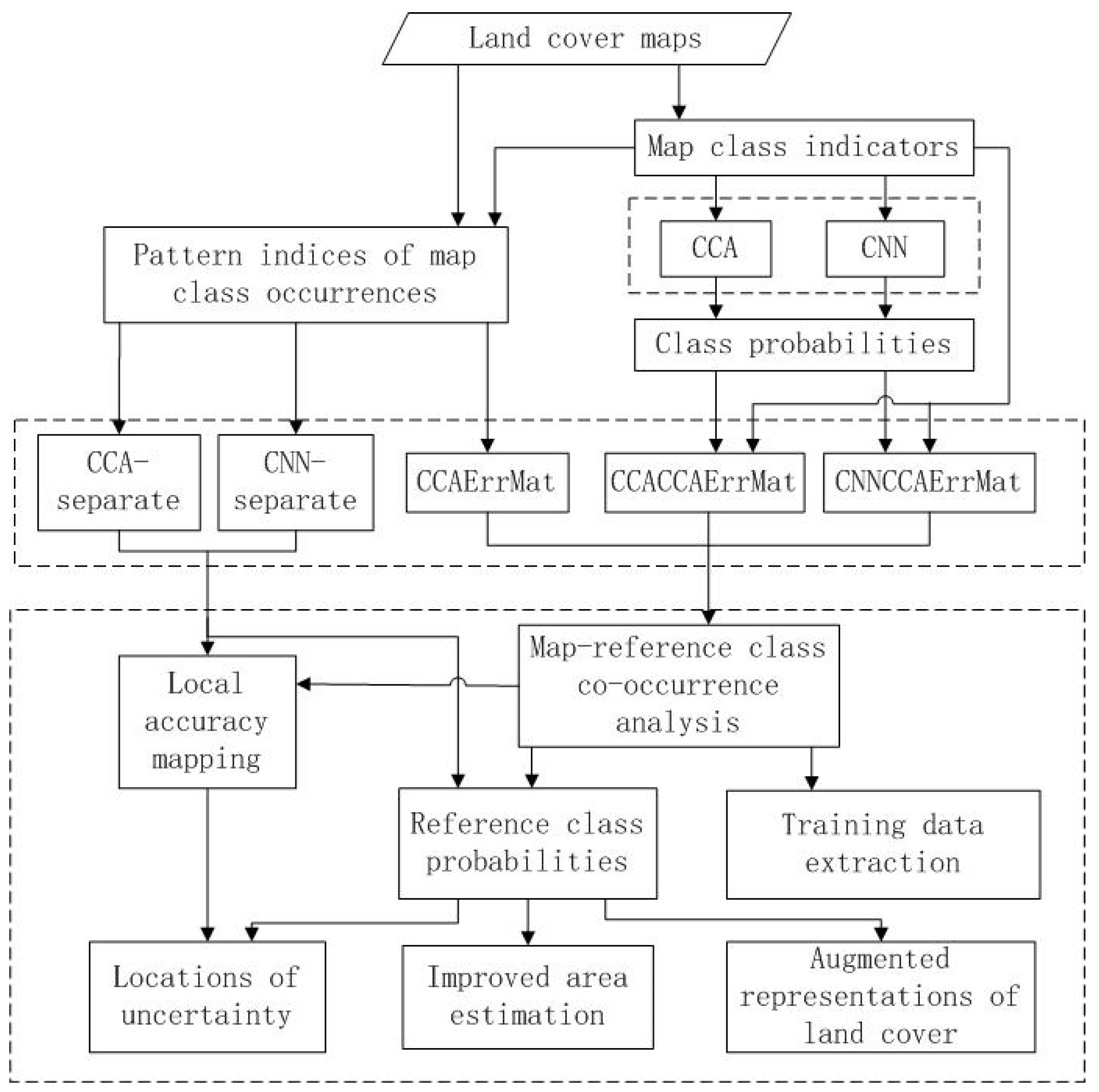
2. Methods
2.1. CCA Feature Space Local Error Matrices: CCAErrMat
2.2. CCA and CNN Used as Feature Extractors for CCAErrMat: CCACCAErrMat and CNNCCAErrMat
2.3. Improved Model-Assisted Area Estimation
3. Experiments
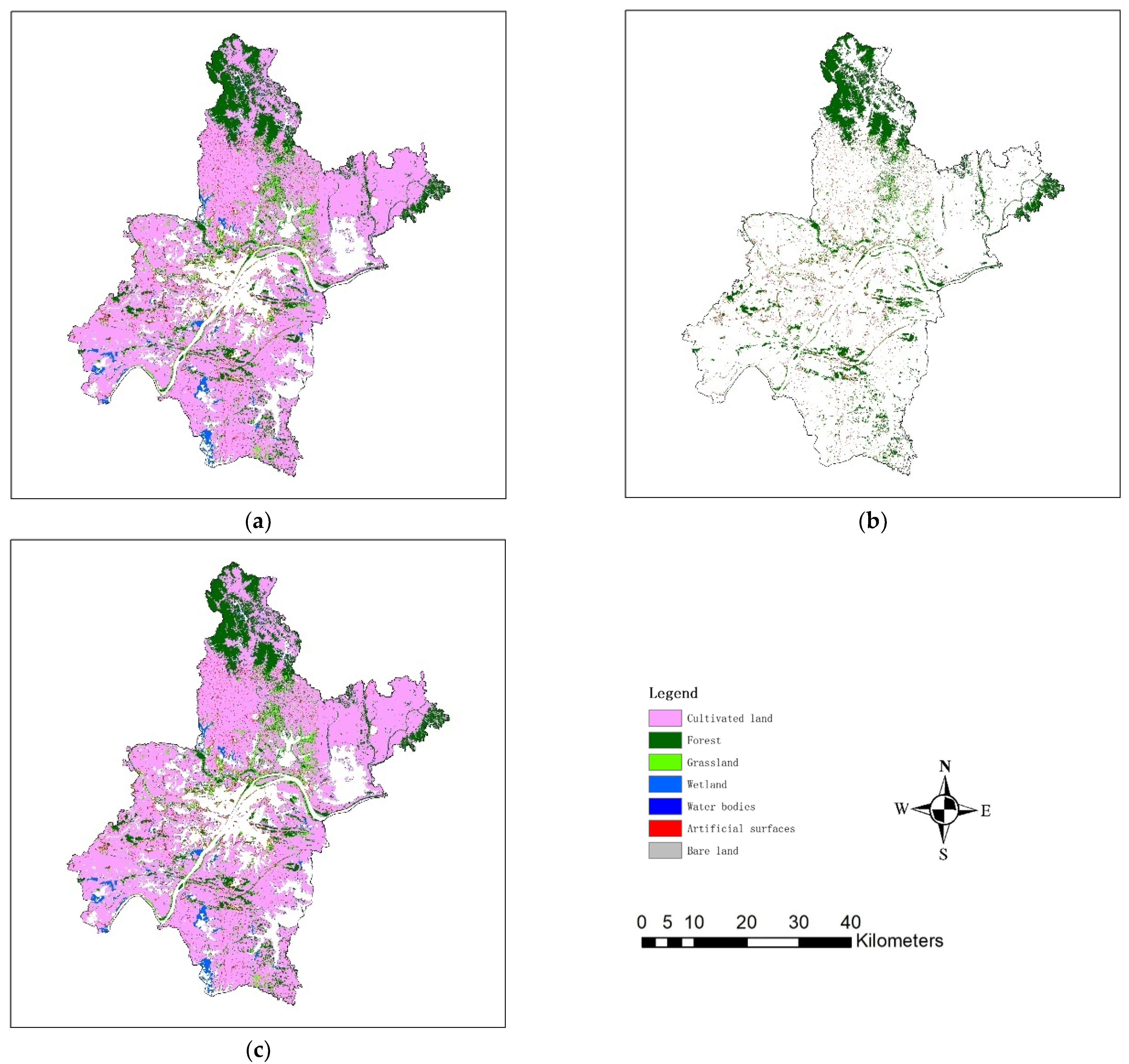
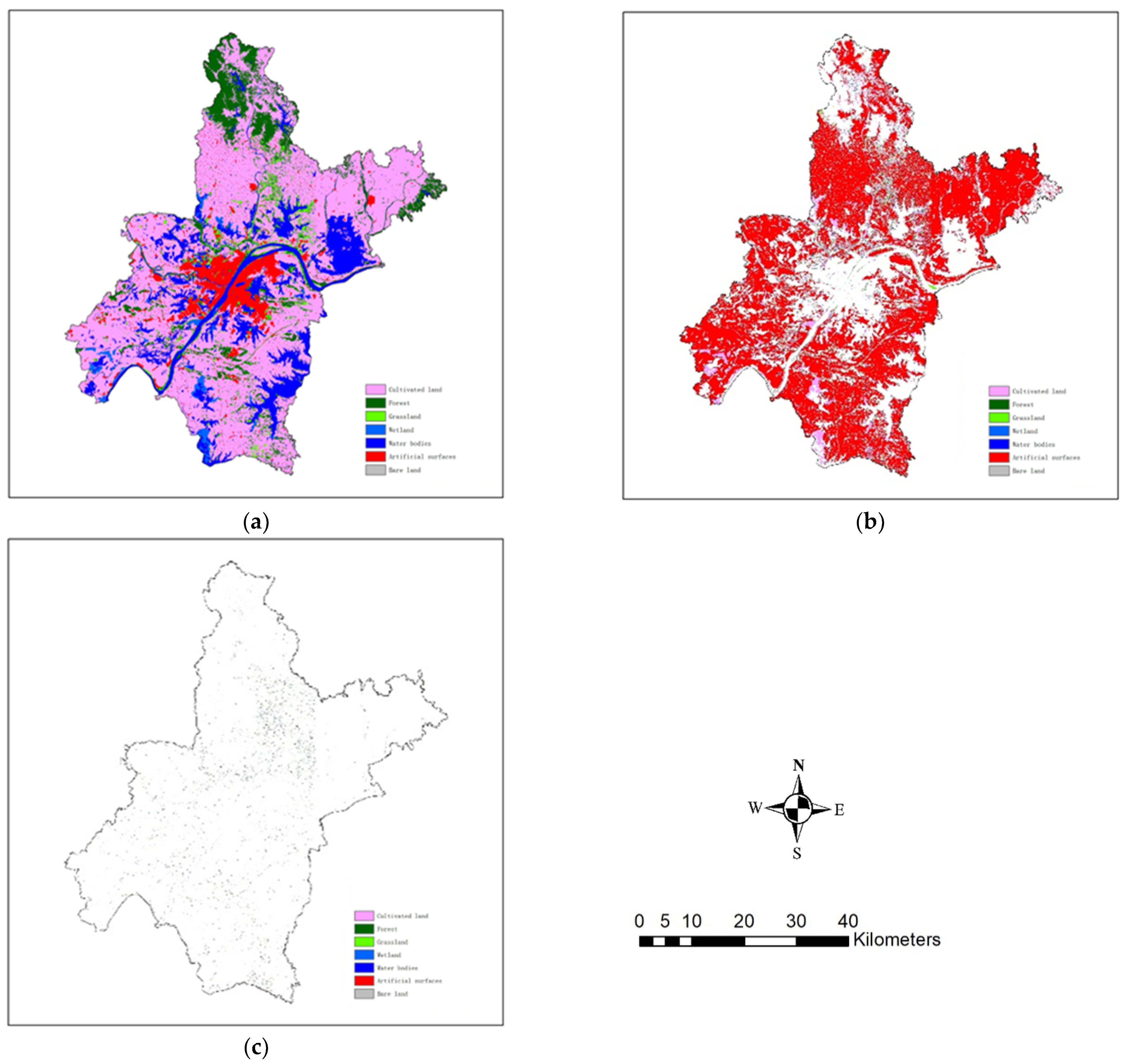
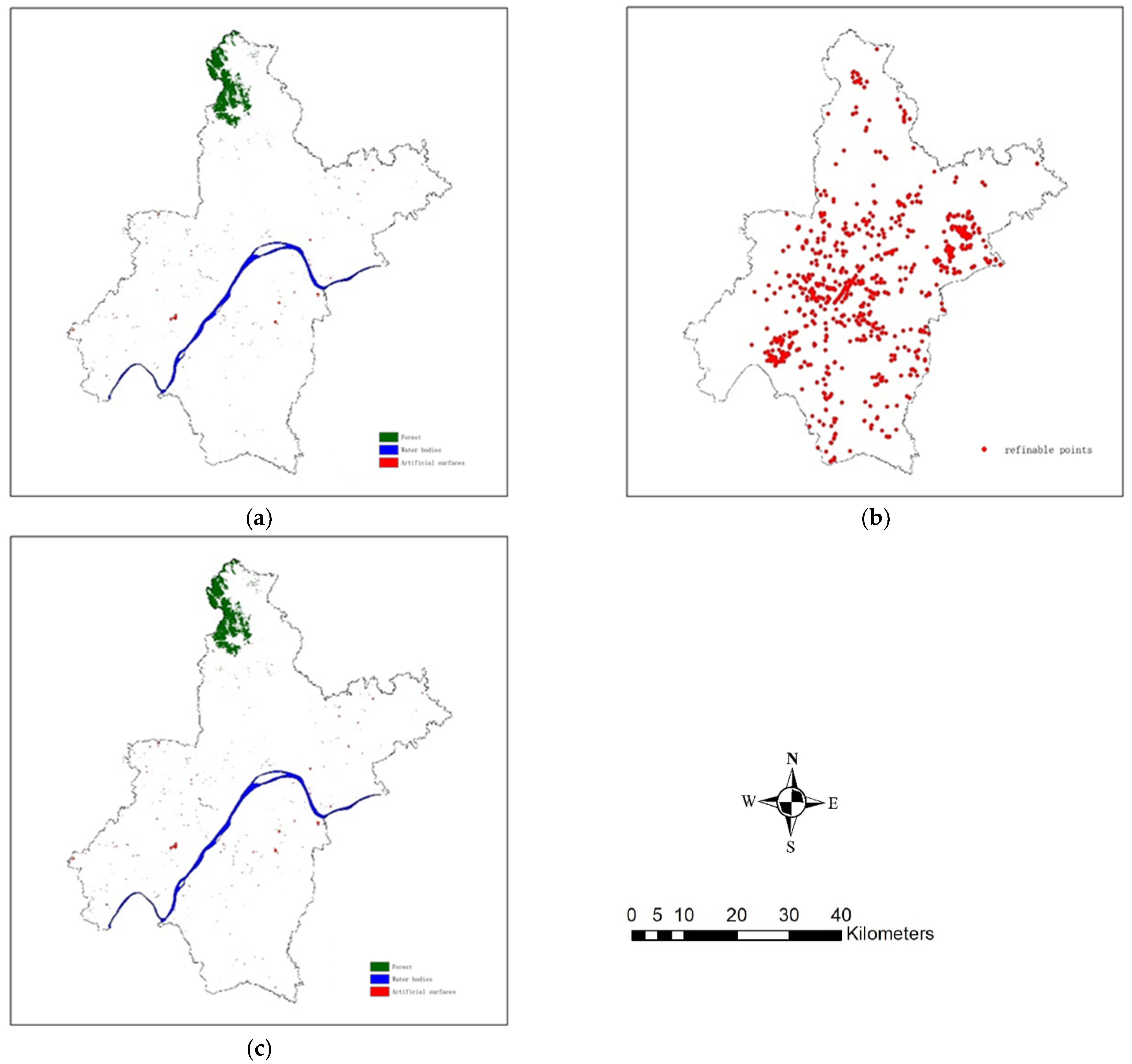
3.1. The Study Site and Datasets
3.2. Results
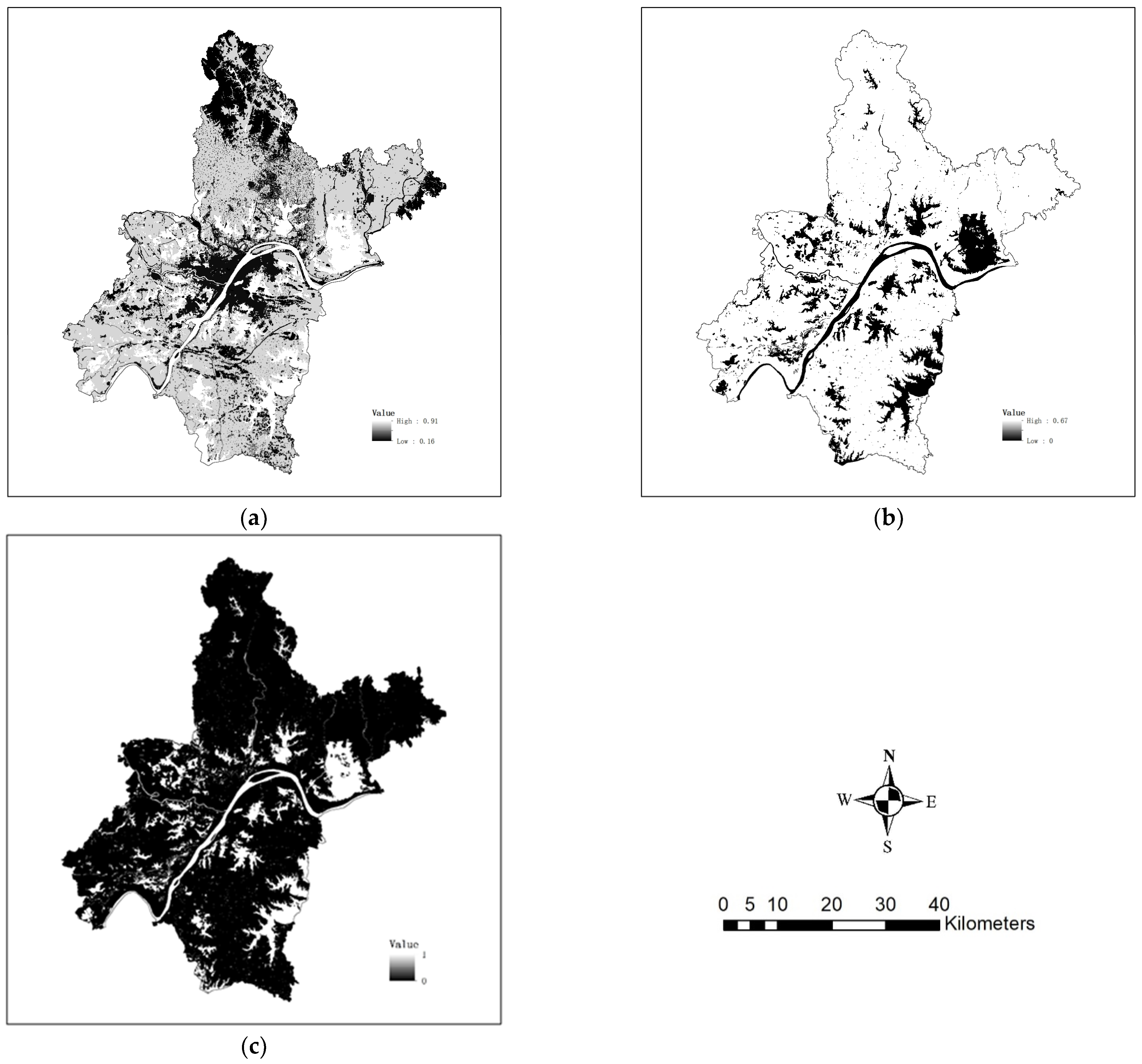
3.2.1. Mapping Local Accuracy
3.2.2. Analyzing Map-Reference Class Co-Occurrences
3.2.3. Improved Area Estimation
4. Discussions
4.1. Comparisons with Related Work
4.2. Recommendation for Further Research
5. Conclusions
Author Contributions
Funding
Data Availability Statement
Conflicts of Interest
Appendix A. CCA Modeling
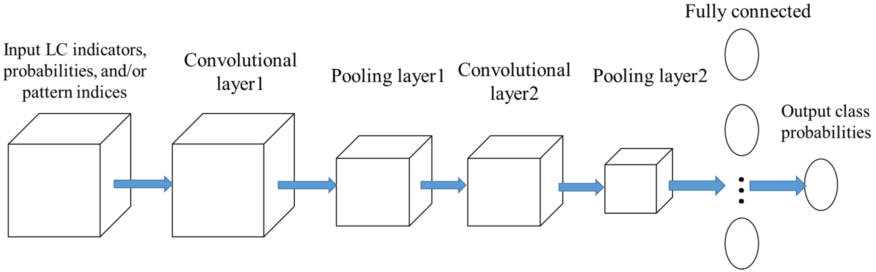
Appendix B. CNN

Appendix C. The π Area Estimator and Some of Model-Assisted Area Estimators
Appendix D. Some of Experiment Results
Appendix D.1. An Error Matrix Estimated for the Original Map

| Map Class | Reference Class | ||||||||
|---|---|---|---|---|---|---|---|---|---|
| Cultivt | Forest | Grass | Wetland | Water | Artfct | Bare | Strata Accuracy | UA | |
| Cultivt (E) | 0.2 | 4.5−2 | 6.4−2 | 3.5−2 | 0.1 | 0.1 | 2.5−2 | 36.7 | 71.8 |
| Cultivt (O) | 43.4 | 2.5 | 1.8 | 2.3 | 5.8 | 3.6 | 0.8 | 72.1 | |
| Forest (E) | 0.3 | 0.4 | 0.2 | 0.1 | 0.4 | 0.1 | 3.0−2 | 26.4 | 73.1 |
| Forest (O) | 0.8 | 8.3 | 0.8 | 0.2 | 0.3 | 0.1 | 3.8−2 | 79.3 | |
| Grass (E) | 0.1 | 0.1 | 0.3 | 3.7−2 | 0.1 | 3.1−2 | 6.1−3 | 38.3 | 48.3 |
| Grass (O) | 0.3 | 0.2 | 1.3 | 4.6−2 | 0.4 | 0.2 | 0.1 | 51.2 | |
| Wetland (E) | 2.7−4 | 0 | 5.3−4 | 1.1−2 | 9.1−3 | 0 | 0 | 53.8 | 69.1 |
| Wetland (O) | 0.1 | 1.0−2 | 2.0−2 | 1.0 | 0.3 | 0 | 0 | 69.3 | |
| Water (E) | 2.3−2 | 7.5−3 | 1.3−2 | 3.0−2 | 0.2 | 0 | 0 | 71.0 | 85.4 |
| Water (O) | 0.4 | 0.1 | 0.6 | 0.6 | 12.5 | 0.1 | 0.4 | 85.6 | |
| Artfct (E) | 2.0−2 | 3.9−2 | 1.6−2 | 0 | 1.6−2 | 0.1 | 6.1−3 | 52.0 | 83.1 |
| Artfct (O) | 0.2 | 0.1 | 0.4 | 0 | 0.1 | 6.2 | 0.4 | 84.0 | |
| Bare (E) | 7.2−3 | 9.6−3 | 8.2−3 | 0 | 4.8−4 | 0 | 1.3−2 | 33.8 | 45.1 |
| Bare (O) | 9.0−3 | 1.2−2 | 1.3−2 | 0 | 1.6−3 | 0 | 3.7−2 | 51.1 | |
| PA | 95.1 | 73.0 | 29.5 | 22.9 | 62.8 | 59.8 | 2.9 | 73.9 | |
Appendix D.2. Variable Selection and Optimum k for k Nearest Neighbors
| Re-mapping | Sample Sets | Selected Variables | k |
| 360 pixels | mapclass1+mapclass2+mapclass3+mapclass4+mapclass5+ | 20 | |
| 1020 pixels | mapclass6+hom3+con3+het3+dom3+ent3+p1w3+p2w3+ | 47 | |
| Local accuracy mapping (360 sample pixels) | Selected Variables | k | |
| OA | ent3+mapclass6+mapclass5+p6w9+mapclass4+p5w7+p2w5 | 43 | |
| UA Cultivt | p6w7 | 3 | |
| UA_Forest | con3+patch5+hom3 | 8 | |
| UA_Grass | con5+patch2 | 10 | |
| UA_Wetland | patch3+patch4+dom3+p5w3+con3+het3+patch1+p2w7 | 7 | |
| UA_Water | p1w7+het5+het7+area+patch3+con9 | 6 | |
| UA_Artfct | p8w3 | 20 | |
| UA_Bare | con5+het5+patch4+dom3+het7+p9w3+ent5+patch2+area+ patch5+patch1+dom7+con3+p6w9+ent3+p2w3+patch3+ hom9+het9+p2w5+p2w7+p1w9+hom3 | 7 | |
| PA Cultivt | mapclass1+p1w3+p1w5+p1w7+p1w9 | 1 | |
| PA_Forest | mapclass2+p1w3+p1w5+p1w7+p1w9 | 1 | |
| PA_Grass | mapclass3+p1w3+p1w5+p1w7+p1w9 | 1 | |
| PA_Wetland | mapclass4+p1w3+p1w5+p1w7+p1w9 | 1 | |
| PA_Water | mapclass5+p1w3+p1w5+p1w7+p1w9 | 1 | |
| PA_Artfct | mapclass6+p1w3+p1w5+p1w7+p1w9 | 1 | |
| PA_Bare | mapclass7+p1w3+p1w5+p1w7+p1w9 | 1 | |
| Local accuracy mapping (1020 sample pixels) | Selected Variables | k | |
| OA | ent3+mapclass5+mapclass6+lsihet2_3+mapclass4+ mapclass1+p6w9+p5w7+POINT_Y+hom9+p5w3+p5w9 | 37 | |
| UA Cultivt | ent3+het3+p5w9+p6w5 | 21 | |
| UA_Forest | hom9+patch5+p3w9+p8w3+con3 | 40 | |
| UA_Grass | p1w5+dom5+dom9+patch2+area | 44 | |
| UA_Wetland | p6w3+patch4+patch3+patch1+p3w9+p1w3 | 36 | |
| UA_Water | p1w3+dom3+p3w5+patch6+p2w3 | 14 | |
| UA_Artfct | patch4+dom3+p8w5+hom3+p8w3 | 19 | |
| UA_Bare | patch3+p1w3+hom5+area | 14 | |
| PA Cultivt | mapclass1+p1w3+p1w5+p1w7+p1w9 | 1 | |
| PA_Forest | mapclass2+p1w3+p1w5+p1w7+p1w9 | 1 | |
| PA_Grass | mapclass3+p1w3+p1w5+p1w7+p1w9 | 1 | |
| PA_Wetland | mapclass4+p1w3+p1w5+p1w7+p1w9 | 1 | |
| PA_Water | mapclass5+p1w3+p1w5+p1w7+p1w9 | 1 | |
| PA_Artfct | mapclass6+p1w3+p1w5+p1w7+p1w9 | 1 | |
| PA_Bare | mapclass7+p1w3+p1w5+p1w7+p1w9 | 1 |
| 360 Sample Pixels | OA | UA Cultivt | UA Forest | UA Grass | UA Wetland | UA Water | UA Artfct | UA Bare |
|---|---|---|---|---|---|---|---|---|
| K | 12 | 8 | 6 | 8 | 10 | 23 | 23 | 7 |
| PA Cultivt | PA Forest | PA Grass | PA Wetland | PA Water | PA Artfct | PA Bare | ||
| K | 6 | 24 | 2 | 1 | 5 | 1 | 5 | |
| 1020 Sample Pixels | OA | UA Cultivt | UA Forest | UA Grass | UA Wetland | UA Water | UA Artfct | UA Bare |
| K | 42 | 50 | 22 | 2 | 48 | 12 | 46 | 48 |
| PA Cultivt | PA Forest | PA Grass | PA Wetland | PA Water | PA Artfct | PA Bare | ||
| k | 1 | 24 | 2 | 1 | 5 | 1 | 5 |
References
- Chen, J.; Chen, J.; Liao, A.; Cao, X.; Chen, L.; Chen, X.; He, C.; Han, G.; Peng, S.; Lu, M.; et al. Global land cover mapping at 30 m resolution: A POK-based operational approach. ISPRS J. Photogramm. Remote Sens. 2015, 103, 7–27. [Google Scholar] [CrossRef] [Green Version]
- Brown, J.F.; Tollerud, H.J.; Barber, C.P.; Zhou, Q.; Dwyer, J.L.; Vogelmann, J.E.; Loveland, T.R.; Woodcock, C.E.; Stehman, S.V.; Zhu, Z.; et al. Lessons learned implementing an operational continuous United States national land change monitoring capability—The Land Change Monitoring, Assessment, and Projection (LCMAP) approach. Remote Sens. Environ. 2020, 238, 111356. [Google Scholar] [CrossRef]
- Buchhorn, M.; Lesiv, M.; Tsendbazar, N.-E.; Herold, M.; Bertels, L.; Smets, B. Copernicus global land cover layers-collection 2. Remote Sens. 2020, 12, 1044. [Google Scholar] [CrossRef] [Green Version]
- Friedl, M.A.; McIver, D.K.; Hodges, J.C.F.; Zhang, X.Y.; Muchoney, D.; Strahler, A.H.; Woodcock, C.E.; Gopal, S.; Schneider, A.; Cooper, A.; et al. Global land cover mapping from MODIS: Algorithms and early results. Remote Sens. Environ. 2002, 83, 287–302. [Google Scholar] [CrossRef]
- Sulla-Menashe, D.; Gray, J.M.; Abercrombie, S.P.; Friedl, M.A. Hierarchical mapping of annual global land cover 2001 to present: The MODIS collection 6 land cover product. Remote Sens. Environ. 2019, 222, 183–194. [Google Scholar] [CrossRef]
- Yang, Y.; Xiao, P.; Feng, X.; Li, H. Accuracy assessment of seven global land cover datasets over China. ISPRS J. Photogramm. Remote Sens. 2017, 125, 156–173. [Google Scholar] [CrossRef]
- Hua, T.; Zhao, W.; Liu, Y.; Wang, S.; Yang, S. Spatial consistency assessments for global land-cover datasets: A comparison among GLC2000, CCI LC, MCD12, GLOBCOVER and GLCNMO. Remote Sens. 2018, 10, 1846. [Google Scholar] [CrossRef] [Green Version]
- Stehman, S.V. Estimating area from an accuracy assessment error matrix. Remote Sens. Environ. 2013, 132, 202–211. [Google Scholar] [CrossRef]
- Ebrahimy, H.; Mirbagheri, B.; Matkan, A.A.; Azadbakht, M. Per-pixel land cover accuracy prediction: A random forest-based method with limited reference sample data. ISPRS J. Photogramm. Remote Sens. 2021, 172, 17–27. [Google Scholar] [CrossRef]
- Smith, J.H.; Stehman, S.V.; Wickham, J.D.; Yang, L. Effects of landscape characteristics on land-cover class accuracy. Remote Sens. Environ. 2003, 84, 342–349. [Google Scholar] [CrossRef]
- Foody, G.M. Local characterization of thematic classification accuracy through spatially constrained confusion matrices. Int. J. Remote Sens. 2005, 26, 1217–1228. [Google Scholar] [CrossRef]
- Khatami, R.; Mountrakis, G.; Stehman, S.V. Mapping per-pixel predicted accuracy of classified remote sensing images. Remote Sens. Environ. 2017, 191, 156–167. [Google Scholar] [CrossRef] [Green Version]
- Wickham, J.; Stehman, S.V.; Homer, C.G. Spatial patterns of the United States National Land Cover Dataset (NLCD) land-cover change thematic accuracy (2001-2011). Int. J. Remote Sens. 2018, 39, 1729–1743. [Google Scholar] [CrossRef] [Green Version]
- Stehman, S.V.; Foody, G.M. Key issues in rigorous accuracy assessment of land cover products. Remote Sens. Environ. 2019, 231, 111199. [Google Scholar] [CrossRef]
- Zhang, J.; Zhang, W.; Mei, Y.; Yang, W. Geostatistical characterization of local accuracies in remotely sensed land cover change categorization with complexly configured reference samples. Remote Sens. Environ. 2019, 223, 63–81. [Google Scholar] [CrossRef]
- Steele, B.M.; Winne, J.C.; Redmond, R.L. Estimation and mapping of misclassification probabilities for thematic land cover maps. Remote Sens. Environ. 1998, 66, 192–202. [Google Scholar] [CrossRef]
- Van Oort, P.A.J.; Bregt, A.K.; De Bruin, S.; De Wit, A.J.W.; Stein, A. Spatial variability in classification accuracy of agricultural crops in the Dutch national land-cover database. Int. J. Geogr. Inf. Sci. 2004, 18, 611–626. [Google Scholar] [CrossRef]
- Burnicki, A.C. Modeling the probability of misclassification in a map of land cover change. Photogramm. Eng. Remote Sens. 2011, 77, 39–50. [Google Scholar] [CrossRef]
- Comber, A.; Brunsdon, C.; Charlton, M.; Harris, P. Geographically weighted correspondence matrices for local error reporting and change analyses: Mapping the spatial distribution of errors and change. Remote Sens. Lett. 2017, 8, 234–243. [Google Scholar] [CrossRef] [Green Version]
- Huang, X.; Song, Y.H.; Yang, J.; Wang, W.R.; Ren, H.Q.; Dong, M.J.; Feng, Y.J.; Yin, H.D.; Li, J.Y. Toward accurate mapping of 30-m time-series global impervious surface area (GISA). Int. J. Appl. Earth Obs. Geoinf. 2022, 109, 102787. [Google Scholar] [CrossRef]
- Wan, Y.; Zhang, J.; Yang, W.; Tang, Y. Refining land-cover maps based on probabilistic re-classification in CCA ordination space. Remote Sens. 2020, 12, 2954. [Google Scholar] [CrossRef]
- Campos, J.C.; Brito, J.C. Mapping underrepresented land cover heterogeneity in arid regions: The Sahara-Sahel example. ISPRS J. Photogramm. Remote Sens. 2018, 146, 211–220. [Google Scholar] [CrossRef]
- Zhang, W.L.; Wang, J.W.; Lin, H.T.; Cong, M.; Wan, Y.; Zhang, J.X. Fusing multiple land cover products based on locally estimated map-reference cover type transition probabilities. Remote Sens. 2023, 15, 481. [Google Scholar] [CrossRef]
- Olofsson, P.; Foody, G.M.; Herold, M.; Stehman, S.V.; Woodcock, C.E.; Wulder, M.A. Good practices for estimating area and assessing accuracy of land change. Remote Sens. Environ. 2014, 148, 42–57. [Google Scholar] [CrossRef]
- Breidt, F.J.; Opsomer, J.D. Model-assisted survey estimation with modern prediction techniques. Stat. Sci. 2017, 32, 190–205. [Google Scholar] [CrossRef]
- McConville, K.S.; Moisen, G.G.; Frescino, T.S. A tutorial on model-assisted estimation with application to forest inventory. Forests 2020, 11, 244. [Google Scholar] [CrossRef] [Green Version]
- Ter Braak, C.J. The analysis of vegetation-environment relationships by canonical correspondence analysis. Vegetatio 1987, 69, 69–77. [Google Scholar] [CrossRef]
- Legendre, P.; Legendre, L. Numerical Ecology; Elsevier: Amsterdam, The Netherlands, 2012. [Google Scholar]
- Crookston, N.L.; Finley, A.O. yaImpute: An R Package for kNN Imputation. J. Stat. Softw. 2008, 23, 1–16. [Google Scholar] [CrossRef] [Green Version]
- Duveneck, M.J.; Thompson, J.R.; Wilson, B.T. An imputed forest composition map for New England screened by species range boundaries. For. Ecol. Manage 2015, 347, 107–115. [Google Scholar] [CrossRef]
- McRoberts, R.E.; Næsset, E.; Gobakken, T. Optimizing the k-Nearest neighbors technique for estimating forest aboveground biomass using airborne laser scanning data. Remote Sens. Environ. 2015, 163, 13–22. [Google Scholar] [CrossRef]
- Xu, C.; Manley, B.; Morgenroth, J. Evaluation of modelling approaches in predicting forest volume and stand age for small-scale plantation forests in New Zealand with RapidEye and LiDAR. Int. J. Appl. Earth Obs. Geoinf. 2018, 73, 386–396. [Google Scholar] [CrossRef]
- Feilhauer, H.; Zlinsky, A.; Kania, A.; Foody, G.M.; Doktor, D.; Lausch, A.; Schmidtlein, S. Let your maps be fuzzy!—Class probabilities and floristic gradients as alternatives to crisp mapping for remote sensing of vegetation. Remote Sens. Ecol. Conserv. 2020, 7, 292–305. [Google Scholar] [CrossRef]
- McGarigal, K.; Tagil, S.; Cushman, S.A. Surface metrics: An alternative to patch metrics for the quantification of landscape structure. Landsc. Ecol. 2009, 24, 433–450. [Google Scholar] [CrossRef]
- O’Neill, R.V.; Krummel, J.R.; Gardner, R.H.; Sugihara, G.; Jackson, B.; DeAngelis, D.L.; Milne, B.T.; Turner, M.G.; Zygmunt, B.; Christensen, S.W.; et al. Indices of landscape pattern. Landsc. Ecol. 1988, 1, 153–162. [Google Scholar] [CrossRef]
- Riitters, K.H.; O’Neill, R.V.; Wickham, J.D. A note on contagion indices for landscape analysis. Landsc. Ecol. 1996, 11, 197–202. [Google Scholar] [CrossRef]
- Särndal, C.E.; Swensson, B.; Wretman, J. Model-Assisted Survey Sampling; Springer: New York, NY, USA, 1992. [Google Scholar]
- Ståhl, G.; Saarela, S.; Schnell, S.; Holm, S.; Breidenbach, J.; Healey, S.P.; Patterson, P.L.; Magnussen, S.; Næsset, E.; McRoberts, R.E.; et al. Use of models in large-area forest surveys: Comparing model-assisted, model-based and hybrid estimation. For. Ecosyst. 2016, 3, 5. [Google Scholar] [CrossRef] [Green Version]
- Pickering, J.; Stehman, S.V.; Tyukavina, A.; Potapov, P.; Watt, P.; Jantz, S.M.; Bholanath, P.; Hansen, M.C. Quantifying the trade-off between cost and precision in estimating area of forest loss and degradation using probability sampling in Guyana. Remote Sens. Environ. 2019, 221, 122–135. [Google Scholar] [CrossRef]
- Zhang, J.; Yang, W.; Zhang, W.; Wang, Y.; Liu, D.; Xiu, Y. An explorative study on estimating local accuracies in land-cover information using logistic regression and class-heterogeneity-stratified data. Remote Sens. 2018, 10, 1581. [Google Scholar] [CrossRef] [Green Version]
- Sweeney, S.P.; Evans, T.P. An edge-oriented approach to thematic map error assessment. Geocarto Int. 2012, 27, 31–56. [Google Scholar] [CrossRef]
- Hanley, J.A.; McNeil, B.J. A method of comparing the areas under receiver operating characteristic curves derived from the same cases. Radiology 1983, 148, 839–843. [Google Scholar] [CrossRef] [Green Version]
- Yu, L.; Liu, X.; Zhao, Y.; Yu, C.; Gong, P. Difficult to map regions in 30 m global land cover mapping determined with a common validation dataset. Int. J. Remote Sens. 2018, 39, 4077–4087. [Google Scholar] [CrossRef]
- Sales, M.H.R.; De Bruin, S.; Souza, C.; Herold, M. Land use and land cover area estimates from class membership probability of a random forest classification. IEEE Trans. Geosci. Remote Sens. 2022, 60, 4402711. [Google Scholar] [CrossRef]
- Jung, M.; Henkel, K.; Herold, M.; Churkina, G. Exploiting synergies of global land cover products for carbon cycle modeling. Remote Sens. Environ. 2006, 101, 534–553. [Google Scholar] [CrossRef]
- Iwao, K.; Nasahara, K.N.; Kinoshita, T.; Yamagata, Y.; Patton, D.; Tsuchida, S. Creation of new global land cover map with map integration. J. Geogr. Inf. Syst. 2011, 3, 160–165. [Google Scholar] [CrossRef] [Green Version]
- Tuanmu, M.-N.; Jetz, W. A global 1-km consensus land-cover product for biodiversity and ecosystem modelling. Glob. Ecol. Biogeogr. 2014, 23, 1031–1045. [Google Scholar] [CrossRef]
- See, L.; Schepaschenko, D.; Lesiv, M.; Kraxner, F.; Obersteiner, M. Building a hybrid land cover map with crowdsourcing and geographically weighted regression. ISPRS J. Photogramm. Remote Sens. 2015, 103, 48–56. [Google Scholar] [CrossRef] [Green Version]
- Gengler, S.; Bogaert, P. Combining land cover products using a minimum divergence and a Bayesian data fusion approach. Int. J. Geogr. Inf. Sci. 2018, 32, 806–826. [Google Scholar] [CrossRef]
- Pérez-Hoyos, A.; Udías, A.; Rembold, F. Integrating multiple land cover maps through a multi-criteria analysis to improve agricultural monitoring in Africa. Int. J. Appl. Earth Obs. Geoinf. 2020, 88, 102064. [Google Scholar] [CrossRef]
- Li, Z.; White, J.C.; Wulder, M.A.; Hermosilla, T.; Davidson, A.M.; Comber, A.J. Land cover harmonization using Latent Dirichlet Allocation. Int. J. Geogr. Inf. Sci. 2021, 35, 348–374. [Google Scholar] [CrossRef]
- Saah, D.; Tenneson, K.; Poortinga, A.; Nguyen, Q.; Chishtie, F.; Aung, K.S.; Markert, K.N.; Clinton, N.; Anderson, E.R.; Cutter, P.; et al. Primitives as building blocks for constructing land cover maps. Int. J. Appl. Earth Obs. Geoinf. 2020, 85, 101979. [Google Scholar] [CrossRef]
- Healey, S.P.; Cohen, W.B.; Yang, Z.; Brewer, C.K.; Brooks, E.B.; Gorelick, N.; Hernandez, A.J.; Huang, C.; Hughes, M.J.; Kennedy, R.E.; et al. Mapping forest change using stacked generalization: An ensemble approach. Remote Sens. Environ. 2018, 204, 717–728. [Google Scholar] [CrossRef]
- Chughtai, A.H.; Abbasi, H.; Karas, I.R. A review on change detection method and accuracy assessment for land use land cover. Remote Sens. Appl. Soc. Environ. 2021, 22, 100482. [Google Scholar] [CrossRef]
- Xu, L.; Herold, M.; Tsendbazar, N.-E.; Masiliūnas, D.; Li, L.; Lesiv, M.; Fritz, S.; Verbesselt, J. Time series analysis for global land cover change monitoring: A comparison across sensors. Remote Sens. Environ. 2022, 271, 112905. [Google Scholar] [CrossRef]
- Olofsson, P.; Arévalo, P.; Espejo, A.B.; Green, C.; Lindquist, E.; McRoberts, R.E.; Sanz, M.J. Mitigating the effects of omission errors on area and area change estimates. Remote Sens. Environ. 2020, 236, 111492. [Google Scholar] [CrossRef]
- Masiliūnas, D.; Tsendbazar, N.E.; Herold, M.; Lesiv, M.; Buchhorn, M.; Verbesselt, J. Global land characterisation using land cover fractions at 100 m resolution. Remote Sens. Environ. 2021, 259, 112409. [Google Scholar] [CrossRef]
- Silván-Cárdenas, J.L.; Wang, L. Sub-pixel confusion-uncertainty matrix for assessing soft classifications. Remote Sens. Environ. 2008, 112, 1081–1095. [Google Scholar] [CrossRef]
- Carranza-García, M.; García-Gutiérrez, J.; Riquelme, J.C. A framework for evaluating land use and land cover classification using convolutional neural networks. Remote Sens. 2019, 11, 274. [Google Scholar] [CrossRef] [Green Version]
- McConville, K.; Tang, B.; Zhu, G.; Cheung, S.; Li, S. Mase: Model-Assisted Survey Estimation, Version 0.1.3. 2018; Available online: https://cran.r-project.org/package=mase (accessed on 26 February 2023).
- Lumley, T. Survey: Analysis of complex survey samples, R package version 4.0. J. Stat. Softw. 2020, 9, 1–19. [Google Scholar]
- Ma, Z.; Redmond, R.L. Tau coefficients for accuracy assessment of classification of remote sensing data. Photogramm. Eng. Remote Sens. 1995, 61, 435–439. [Google Scholar]


| Strata and Sub-Strata | Nstrata | Training Sample Full Set (Sampling Intensity) | Sample Subset I | Sample Subset II | Test Sample Full Set (Sampling Intensity) | Sample Subset III |
|---|---|---|---|---|---|---|
| Cultivt_E | 56,721 | 120 (0.21) | 15 | 60 | 60 (0.11) | 15 |
| Cultivt_O | 5,739,203 | 1095 (0.02) | 132 | 160 | 160 (0.003) | 132 |
| Forest_E | 133,655 | 140 (0.10) | 18 | 70 | 70 (0.05) | 18 |
| Forest_O | 1,001,767 | 280 (0.03) | 27 | 100 | 100 (0.01) | 27 |
| Grass_E | 70,366 | 120 (0.17) | 15 | 60 | 60 (0.09) | 15 |
| Grass_O | 248,912 | 170 (0.07) | 21 | 80 | 80 (0.03) | 21 |
| Wetland_E | 2033 | 80 (3.93) | 9 | 40 | 40 (1.97) | 9 |
| Wetland_O | 133,735 | 140 (0.10) | 18 | 70 | 70 (0.05) | 18 |
| Water_E | 23,895 | 100 (0.42) | 12 | 50 | 50 (0.21) | 12 |
| Water_O | 1,395,043 | 285 (0.02) | 33 | 110 | 110 (0.01) | 33 |
| Artfct_E | 19,324 | 100 (0.52) | 12 | 50 | 50 (0.26) | 12 |
| Artfct_O | 699,787 | 200 (0.03) | 24 | 90 | 90 (0.01) | 24 |
| Bare_E | 3658 | 80 (2.19) | 12 | 40 | 40 (1.10) | 12 |
| Bare_O | 6994 | 90 (1.29) | 12 | 40 | 40 (0.58) | 12 |
| All | 9,535,093 | 3000 | 360 | 1020 | 1020 | 360 |
| CCAErrMat | CCA-Separate | CNN-Separate | CCACCAErrMat | CNNCCAErrMat | |||||||
|---|---|---|---|---|---|---|---|---|---|---|---|
| 360 | 1020 | 360 | 1020 | 360 | 1020 | 360 | 1020 | 360 | 1020 | ||
| Local OA | 0.71 | 0.72 | 0.75 | 0.79 | 0.74 | 0.77 | 0.74 | 0.77 | 0.72 | 0.76 | |
| Local UA | Cultivt | 0.72 | 0.71 | 0.67 | 0.75 | 0.78 | 0.75 | 0.70 | 0.74 | 0.62 | 0.76 |
| Forest | 0.79 | 0.83 | 0.78 | 0.87 | 0.82 | 0.86 | 0.77 | 0.82 | 0.82 | 0.87 | |
| Grass | 0.61 | 0.50 | 0.57 | 0.54 | 0.66 | 0.61 | 0.67 | 0.65 | 0.61 | 0.56 | |
| Wetland | 0.61 | 0.68 | 0.61 | 0.71 | 0.40 | 0.70 | 0.54 | 0.67 | 0.36 | 0.70 | |
| Water | 0.45 | 0.62 | 0.66 | 0.81 | 0.55 | 0.54 | 0.56 | 0.56 | 0.54 | 0.54 | |
| Artfct | 0.70 | 0.56 | 0.69 | 0.66 | 0.73 | 0.71 | 0.71 | 0.70 | 0.69 | 0.70 | |
| Bare | 0.63 | 0.65 | 0.58 | 0.80 | 0.72 | 0.87 | 0.62 | 0.70 | 0.73 | 0.79 | |
| Local PA | Cultivt | 1.00 | 1.00 | 1.00 | 1.00 | 0.99 | 1.00 | 1.00 | 1.00 | 1.00 | 1.00 |
| Forest | 1.00 | 1.00 | 1.00 | 1.00 | 0.99 | 1.00 | 1.00 | 1.00 | 1.00 | 1.00 | |
| Grass | 1.00 | 1.00 | 1.00 | 1.00 | 0.98 | 1.00 | 1.00 | 1.00 | 1.00 | 1.00 | |
| Wetland | 1.00 | 1.00 | 1.00 | 1.00 | 1.00 | 1.00 | 1.00 | 1.00 | 1.00 | 1.00 | |
| Water | 0.99 | 0.99 | 1.00 | 1.00 | 0.99 | 1.00 | 1.00 | 1.00 | 1.00 | 1.00 | |
| Artfct | 1.00 | 1.00 | 1.00 | 1.00 | 0.98 | 1.00 | 1.00 | 1.00 | 1.00 | 1.00 | |
| Bare | 0.98 | 1.00 | 1.00 | 1.00 | 0.96 | 1.00 | 1.00 | 1.00 | 1.00 | 1.00 | |
| Area | Cultvt Land | Forest | Grass | Wetland | Water | Artificial Surfaces | Bare Land | |
|---|---|---|---|---|---|---|---|---|
| 360 pixels | π estimator | 50.1 | 12.9 | 6.8 | 3.4 | 17.1 | 8.9 | 0.8 |
| Difference estimator | 50.4 | 12.6 | 6.9 | 3.5 | 16.9 | 8.8 | 0.8 | |
| Regression estimator | 50.4 | 12.6 | 6.9 | 3.6 | 16.9 | 8.8 | 0.8 | |
| 1020 pixels | π estimator | 49.1 | 12.6 | 6.7 | 2.6 | 19.5 | 8.9 | 0.6 |
| Difference estimator | 49.9 | 12.6 | 6.5 | 2.5 | 18.9 | 9.1 | 0.6 | |
| Regression estimator | 50.0 | 12.6 | 6.5 | 2.6 | 18.7 | 9.1 | 0.6 |
| SE | Cultvt Land | Forest | Grass | Wetland | Water | Artificial Surfaces | Bare Land | |
|---|---|---|---|---|---|---|---|---|
| 360 pixels | π estimator | 5.0 | 14.1 | 24.0 | 38.3 | 12.4 | 18.3 | 102.4 |
| Difference estimator | 3.9 | 11.6 | 21.7 | 28.1 | 8.9 | 12.8 | 91.5 | |
| Regression estimator | 3.8 | 11.6 | 21.7 | 28.2 | 8.7 | 12.8 | 96.5 | |
| 1020 pixels | π estimator | 2.6 | 8.9 | 16.1 | 32.2 | 7.0 | 12.0 | 81.9 |
| Difference estimator | 2.1 | 6.8 | 15.0 | 26.5 | 5.1 | 7.4 | 78.7 | |
| Regression estimator | 2.0 | 6.8 | 15.0 | 26.0 | 5.1 | 7.5 | 80.6 |
Disclaimer/Publisher’s Note: The statements, opinions and data contained in all publications are solely those of the individual author(s) and contributor(s) and not of MDPI and/or the editor(s). MDPI and/or the editor(s) disclaim responsibility for any injury to people or property resulting from any ideas, methods, instructions or products referred to in the content. |
© 2023 by the authors. Licensee MDPI, Basel, Switzerland. This article is an open access article distributed under the terms and conditions of the Creative Commons Attribution (CC BY) license (https://creativecommons.org/licenses/by/4.0/).
Share and Cite
Wan, Y.; Zhang, J.; Zhang, W.; Zhang, Y.; Yang, W.; Wang, J.; Chukwunonso, O.S.; Nadeeka, A.M.T. Characterizing Uncertainty and Enhancing Utility in Remotely Sensed Land Cover Using Error Matrices Localized in Canonical Correspondence Analysis Ordination Space. Remote Sens. 2023, 15, 1367. https://doi.org/10.3390/rs15051367
Wan Y, Zhang J, Zhang W, Zhang Y, Yang W, Wang J, Chukwunonso OS, Nadeeka AMT. Characterizing Uncertainty and Enhancing Utility in Remotely Sensed Land Cover Using Error Matrices Localized in Canonical Correspondence Analysis Ordination Space. Remote Sensing. 2023; 15(5):1367. https://doi.org/10.3390/rs15051367
Chicago/Turabian StyleWan, Yue, Jingxiong Zhang, Wangle Zhang, Ying Zhang, Wenjing Yang, Jianxu Wang, Okafor Somtoochukwu Chukwunonso, and Asurapplullige Milani Tharuka Nadeeka. 2023. "Characterizing Uncertainty and Enhancing Utility in Remotely Sensed Land Cover Using Error Matrices Localized in Canonical Correspondence Analysis Ordination Space" Remote Sensing 15, no. 5: 1367. https://doi.org/10.3390/rs15051367